The Cash Paradox
∗
Janet Hua Jiang
†Bank of Canada
Enchuan Shao
‡University of Saskatchewan
March 15, 2019
Abstract
In many industrialized countries, cash usage at points of sale has been decreasing ow-ing to competition from alternative means of payment such as credit cards. At the same time, cash demand, measured as currency in circulation over GDP, fell only in earlier years but has remained surprisingly robust in the past two to three decades. This phe-nomenon, termed the “cash paradox,” poses a challenge to standard monetary models. We introduce two new features into the standard cash-credit model: the substitutability between cash and credit (as a stand-in for alternative means of payments) is uneven across different economic activities, and some agents actively manage cash flows across these activities. Calibration exercises show that the cash-flow channel is important for quan-titatively capturing the diverging trends in cash usage and demand. There is also some empirical support for our model’s prediction on cash velocity in the retail sector.
JEL codes: E41, E51
Keywords: Demand for Cash, Credit, Velocity, Cash Management
∗For their comments and discussions, we would like to thank the anonymous referee, the Associate Editor,
the Editor, Jonathan Chiu, Ben Fung, Pedro Gomis-Porqueras, Scott Hendry, Miguel Molico, Hector Perez-Saiz, Lukasz Pomorski, Francisco Rivadeneyra, Gerald Stuber, Liang Wang, Russell Wong, and Randall Wright, as well as participants at the African Search and Match Workshop in Marrakesh, the Spring 2014 Midwest Macro Meeting, the 2014 Chicago Fed Summer Workshop, the 2015 Econometric Society World Congress in Montreal, and seminars at the Bank of Canada, the University of Hawaii, the University of Iowa, the University of Saskatchewan, and the University of Windsor. The views expressed in the paper are those of the authors. No responsibility for them should be attributed to the Bank of Canada.
1
Introduction
The retail payment landscape has undergone significant changes in the past few decades with
the emergence of various new payment instruments. As a result, cash has been losing ground
to other means of payment at the point of sale. These developments can potentially impact
the demand for government currency. Given that currency in circulation (CIC) constitutes a
significant share of the balance sheet of a central bank, the shrinking demand for currency
will have critical implications on the central bank’s seigniorage revenue, its independence,
and its ability to conduct monetary policy (see Friedman, 1999; King, 1999; Freedman, 2000;
and Fung et al., 2014).1 It is therefore important to monitor and understand the trend in the
demand for cash.
Given that standard monetary models predict that cash usage and demand tend to move
in the same direction, one would naturally expect the demand for cash to decrease as it is
squeezed out by other payment methods at points of sale. However, surprisingly, the demand
for cash, measured as the value of CIC over GDP, after a steady decrease in earlier years, has
remained flat or even increased in the past two to three decades despite continuous declines
in cash usage; this phenomenon has been observed in various industrialized economies (see
Section 2 for more detailed documentation). Rogoff (2002) wonders at the surprising
popu-larity of paper currency in many industrialized economies. Bailey (2009) calls it the “paradox
of banknotes.” Williams (2012) terms this phenomenon of decreasing cash usage and robust
cash demand the “cash paradox.”2
1For example, CIC consisted of 93% of the Federal Reserve’s liabilities in 2007 just before the financial crisis. As a result of large-scale unconventional monetary policies such as quantitative easing, the share of CIC has decreased substantially since the financial crisis. However, CIC still consists of a significant share of the Federal Reserve’s balance sheet. As of the end of 2018, the share was 40%.
In this paper, we document the cash paradox and develop a parsimonious model that is
consistent with the phenomenon. To account for the cash paradox, we introduce two
inno-vations to standard cash-credit monetary models (where credit is a stand-in for alternative
payment methods to cash). The first innovation is that the substitutability between cash and
credit is uneven across different economic activities. Credit directly competes with cash in
many point-of-sale transactions. However, credit is a less-ideal substitute for cash as a store of
value and transactions in the underground economy, in bars and casinos, or in activities where
record-keeping or monitoring technology is not available, where agents desire anonymity, or
where unbanked or underbanked agents are involved. To capture the variation of
substitutabil-ity between cash and credit across different activities, we model a economy with two sectors:
a cash-credit sector and a cash-only sector. The cash-credit sector captures activities where
cash and credit are perfect substitutes for each other as a means of payment. The cash-only
sector captures activities where it is difficult or impossible for credit to replace cash.
The second innovation is the modelling of cash flows across different sectors. In our
model, some agents actively plan their cash inflows and outflows, receiving cash revenues
(in-flows) in the cash-credit sector to finance spending (out(in-flows) in the cash-only sector. Some
examples of these activities are taxi drivers acquiring cash from passengers to dine in
cash-only restaurants, bakeries receiving cash from customers to purchase ingredients at local
farm-ers’ markets, farmers selling produce in cash to pay unbanked temporary workers, firms using
cash revenues to pay suppliers, and all of them retaining some cash revenues as a store of
value.
With these two innovations, our model predicts that higher credit usage initially reduces
both the share of cash transactions and cash demand. However, once credit usage expands
beyond a certain level, the tight connection between cash usage and demand breaks down.
More specifically, agents adjust their cash management practices in response to further credit
expansions, so that the velocity of cash slows down and the demand for cash remains flat
despite further diminishing cash transactions. The intuition is as follows. With more credit
usage in the cash-credit sector, agents who are buyers in that sector lower their cash demand.
This change implies that agents who are sellers in the cash-credit sector will receive fewer
cash revenues or inflows. To finance their purchases or outflows in the cash-only sector, these
agents acquire more cash in advance to make up for the shortfall in cash receipts. The decrease
in cash demand by the first group of agents is offset by the increasing demand by the second
group, so that the total demand for cash remains flat despite shrinking cash transactions. As
for velocity, note that compared with cash acquired by the first group of agents, which is used
in both sectors, cash acquired by the second group of agents has a lower velocity because it
is used only in the cash-only sector. As credit usage expands, there is a redistribution of cash
demand from the first group of agents to the second group, implying that cash with a lower
velocity constitutes a higher fraction of the total demand for cash. As a result, the overall
velocity of cash decreases.
The decoupling of cash usage and demand in response to credit expansions enables our
model to capture the cash paradox successfully. In particular, the simultaneous decrease in
cash usage and robust cash demand in many industrialized countries can be explained as a
result of credit expansions together with falling nominal interest rates.
To quantify the importance of our new two modelling features in capturing the cash
para-dox, we carry out a series of calibration exercises. More specifically, we calibrate our model
and alternative models where these features are absent, to cash usage and demand in four
ad-vanced economies: Australia, Canada, the United Kingdom and the United States. We find
that both modelling features are important in capturing the cash paradox. The standard
mon-etary model, where both features are absent, cannot explain the robust cash demand. The
size of the cash-credit sector relative to the cash-only sector. In contrast, the model with the
cash-flow channel captures the trend in cash usage and demand well in all four countries with
much more reasonable parameterization. We also find some empirical support for our model’s
prediction on the cash velocity in the retail sector.
Our paper contributes to the literature on the cash paradox by developing the first
for-mal model to capture the phenomenon with plausible quantitative results. Our quantitative
exercises also formalize and deepen the popular indicative discussion that attributes the
para-doxical robust demand for cash in the face of credit expansion to increased demand in the
underground economy and/or as a store of value by either domestic or foreign agents, as these
demand categories are less sensitive to competition from other means of payment.3 We
be-lieve that this is an important first step to explain the cash paradox. The cash-only sector in
our model captures these demand categories as economic activities where it is difficult for
credit to replace cash (and our model predicts that cash is increasingly used for activities in
that sector). The next and more challenging step is to identify the forces that can plausibly
counteract the fall in cash demand driven by competition from other means of payment.
The increasing demand in less credit-sensitive activities can result from (1) structural
changes, which cause the money demand curve to shift, and/or (2) decreasing nominal interest
rates, represented by movement along the money demand curve. We think it is unlikely that
structural changes could (fully) account for the cash paradox. In general, there is no evidence
that the underground economy has experienced significant growth. According to Schneider
and Buehn (2012), from 1999 to 2010, the shadow economy as a percentage of GDP shrunk
slightly in 39 OECD countries. Another potential source of structural changes is increased
per-ceived uncertainty and distrust in the financial system, which induce agents to hold more cash
for precautionary motives or as a store of value (see, for example, Williams, 2012; Berentsen
and Schar, 2018). However, in many countries, the cash paradox phenomenon was observed
long before the financial crisis, with the CIC/GDP starting to level off or increase since the
1980s or 1990s. The financial crisis raised perceived uncertainty and distrust in the
finan-cial system and spurred the particularly strong cash demand afterward. Because of that, the
cash paradox phenomenon has drawn more attention following the crisis. However, we think
increased uncertainty and distrust in the financial system are unlikely to be the main force
be-hind the robust cash demand before the financial crisis. Foreign demand could be an important
factor for major international reserve currencies, such as the US dollar or euro. It is, however,
less applicable to other currencies. Given the ubiquity of the cash paradox, country-specific
factors, such as strong foreign demand, are unlikely to fully account for the phenomenon.
The critical question is then whether the fall in the interest rate can plausibly generate
a robust demand for cash as a store of value or in the underground economy to sufficiently
counteract the shrinking (transnational) demand for cash due to expanding credit usage. Our
calibration exercises suggest that the answer is “very unlikely” without additional channels
such as the cash-flow channel proposed in our paper, unless one is willing to make extreme
assumptions about the relative size of the cash-credit sector to the cash-only sector (the former
is less than 1/10,000 of the latter). The cash-flow channel that we emphasize strengthens the
role of the falling interest rate relative to credit expansion, and helps to capture the paradoxical
behavior of cash demand with much more plausible model parameterization.
Our model also closely relates to works that study credit in monetary economies within
the framework developed by Lagos and Wright (2005) and Rocheteau and Wright (2005).
Gu et al. (2016) and Araugo and Hu (2017) discuss the essentiality of credit in a monetary
economy. Berentsen et al. (2007), Rojas Breu (2013), Berentsen et al. (2014), and Chiu et al.
(2010) and Gomis-Porqueras and Sanches (2013) investigate the optimal monetary policy in a
model with money and credit. Bethune et al. (2014) study the relationship between unsecured
consumer credit and unemployment. Lotz and Zhang (2016) and Dong and Huangfu (2017)
model costly credit and examine how monetary policies affect credit adoption. Liu et al.
(2016) analyze the effects of inflation on price dispersion, markups, and welfare.
Our modelling innovation is to introduce cash flows between activities where cash and
credit have different extents of substitutability, and we apply this new model to explain the
paradoxical behavior of cash demand in response to increasing competition from credit usage.
We take a short cut in modelling credit expansion as the increasing fraction of agents having
access to credit (in our Bank of Canada Staff Working Paper version, Jiang and Shao 2014, we
model credit expansion along the intensive margin as increasing credit limits, and the results
are largely the same).4 One could endogenize credit expansion by introducing heterogeneous
preferences and a fixed cost of adopting credit, as in Dong and Huangfu (2017). In this setup,
agents with high marginal utilities tend to use credit. Financial innovations that reduce the
cost of adopting credit will induce more agents to use it. One could also endogenize credit
limits as in Kehoe and Levine (1993), and derive credit expansion along the intensive margin
as higher credit limits resulting from improvements in the monitoring technology to detect
defaults. Endogenizing credit usage would add an interesting interaction between inflation (or
nominal interest rate) and credit adoption or usage. However, given that the data on the cost of
using credit and the monitoring technology are not readily available, in the end, one still needs
to calibrate the cost or monitoring parameter to match observable data on credit adoption or
usage, such as the credit access rate used in our calibration.
Finally, by modelling the cash flows across different sectors where cash and credit have
different substitutability, our model generates a new channel through which credit and the
nominal interest rate affects cash velocity, as apposed to the traditional way of modeling
pre-cautionary demand (as in, for example, Hodrick et al., 1991; Jafarey and Masters, 2003;
Peter-son and Shi, 2004; Lagos and Rocheteau, 2005; Faig and Jerez, 2006; Ennis, 2008 and 2009;
Liu et al., 2011; Nosal 2011; Dong and Jiang, 2014; and Hu et al., 2017).
The rest of the paper is organized as follows. Section 2 documents in more detail the
long-term trend in cash demand and the recent puzzling phenomenon of continued
decreas-ing cash usage and robust cash demand. Section 3 describes the model and characterizes the
equilibrium. Section 4 derives the comparative statics and discusses the effect of credit
ex-pansions and the nominal interest rate on cash usage and demand. In Section 5, we calibrate
three models–the standard single-sector cash-credit model, the segregated two-sector model
where cash and credit have different substitutability across the two sectors, and the full model
where cash flows between the two sectors–to quantify the importance of the modelling
fea-tures. In that section, we also evaluate in detail existing alternative explanations about the cash
paradox and pinpoint the value-added of the cash-flow channel that we emphasize. Section 6
provides empirical support to our model’s predictions on cash velocity. Section 7 concludes.
In the appendices, we provide the proofs, document the data used in our quantitative analysis,
discuss different measures of nominal interest rates, lay out the standard single sector
cash-credit model and the segregated two-sector model for comparison, investigate the possibility
of unregistered economic activities to capture the cash paradox, and discuss model extensions.
2
Documentation of the Cash Paradox
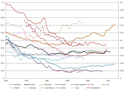
Figure 1 graphs the time series of CIC/GDP ratio for 13 industrialized countries from 1960
and onward: Australia, Canada, Denmark, Iceland, New Zealand, the United Kingdom, the
0 0.02 0.04 0.06 0.08 0.1 0.12 0.14 0.16 0.18 0.2
0 0.01 0.02 0.03 0.04 0.05 0.06 0.07 0.08 0.09 0.1
1960 1970 1980 1990 2000 2010 Australia Canada Denmark Iceland New Zealand UK U.S. Finland Germany Luxembourg Austria Italy Switzerland
Figure 1: Currency in circulation over GDP for selected countries
Notes: (a) Data source: IMF-IFS. (b)The series for Austria, Italy, and Switzerland are plotted against the right y-axis.
Luxembourg, subject to data availability.5 The demand for cash experienced a steady decrease
in earlier years, but the trend has stopped in the last two to three decades, in spite of a continued
decrease in cash usage at points of sales.6
There are in general two approaches to estimating the value of cash transactions. The
first proxies cash usage by cash withdrawals (see, for example, Gerdes et al., 2005) or by the
residual after subtracting non-cash payments from the total point-of-sales or from household
expenditures (see, for example, Humphrey et al., 2004). The second approach directly
cal-culates the share of cash payments from consumer payment survey or retailer scanner data.
Various studies have been conducted to investigate the substitution between cash and other
payment methods in many countries. A common result is that cash has been replaced by other
means of payment (to different extents in different countries).
For example, Arango et al. (2012) find that in Canada from the early 1990s to 2011, the
share of cash transactions at points of sale decreased from 80% to 40% in volume, and from
more than 50% to less than 20% in value. The Bank of Canada conducted two
methods-of-payment surveys, in 2009 and 2013. During the four-year intervening period, the share
of cash payments decreased from 54% to 44% in volume, and from 23% to 22% in value.
In the United States, Humphrey (2004) estimates that from 1980 to 2000, the share of cash
transactions in personal consumption expenditures fell from 33% to 20%. Citing two surveys
of payment method usage at US supermarkets conducted by the Food Marketing Institute,
Humphrey (2004) records that cash accounted for 36% of the value of sales in 1994 but fell
to 29% in 1997 and 17% in 2000. Wang and Wolman (2016) use the scanner data from a
large US discount chain store from April 2010 to March 2013 and find that the fraction of
cash transactions fell at a rate of between 1.3% and 3.3% per year, depending on the size
of transactions. In Australia, the Reserve Bank of Australia (RBA) Payments System Board
Annual Report (2013) shows that from 2004 to 2013, cash usage measured by the value of
cash withdrawals grew much more slowly than household consumption. In addition, RBA
conducted two consumer payment diary studies in 2007 and 2010. According to these studies,
the share of the number and value of cash transactions decreased by 6% and 5%, respectively,
during the three-year span (see Bagnall et al., 2016). In New Zealand, a study by Payments
NZ (2014) shows that cash payments as a percentage of total sales decreased by 10 to 20% in
all social-economic areas in New Zealand from 2006 to 2014.
Similar patterns have been observed in many European countries. Referring to data from
the Payments Council, Bailey (2009) documents that in the United Kingdom, the volume of
cash transactions fell from 87% in 1985 to 60% in 2009. In terms of value, the share decreased
from 9% to 4.2% from 1992 to 2008. In Austria, three payment diary surveys were conducted
in 1996, 2000, and 2005. The data show that in terms of volume, the share of cash payments
decreased from 94.9% in 1996, to 92.9% in 2000, and to 86.1% in 2000. The corresponding
payments accounted for about 80% of total purchases in value, whereas in 2002 the figure
dropped to below 50%. In Italy, Alvarez and Lippi (2009) use the Survey of Household
Income and Wealth to calculate the expenditure share paid with currency. For ATM card
holders, the share decreased from 62% in 1993 to 47% in 2004.7 Snellman et al. (2000) study
the substitution of noncash payment instruments for cash in 10 European countries–Belgium,
Denmark, Finland, France, Germany, Italy, Netherlands, Sweden, Switzerland, and the United
Kingdom–from 1987 to 1996. They find that cash was crowded out in all countries (although
the countries were at different stages of this substitution process).
As its name suggests, the cash paradox poses a challenge to standard monetary models.
Two major factors that affect cash usage and demand is the availability of alternative means
of payment (in this paper, we use credit as a stand-in for these alternatives), and the nominal
interest rate. In standard monetary models, cash usage and demand tend to respond in the
same (negative) direction to changes in credit expansion and the nominal interest rate. In
earlier decades, due to credit expansion and a high nominal interest rate, both cash usage and
cash demand decreased. However, in the past two to three decades, credit continues to expand
but the nominal interest rate starts to drop. The fall in cash transactions means that the effect of
credit expansion dominates, while the rise in cash demand requires the opposite. It is difficult
for standard monetary models to resolve the two conflicted requirements and therefore the
cash paradox.8 In the following sections, we show how we can modify the standard
cash-credit monetary models to resolve the conflict.
7Lippi and Secchi (2009) use the same data set as Alvarez and Lippi (2009), but calculate the cash expenditure ratio for non-durable expenditures. According to their calculation, the share of cash expenditure decreased from 85% in 1993 to 69% in 2004.
3
The Model
In this section, we build a cash-credit monetary model based on the framework by Lagos and
Wright (2005) and Rocheteau and Wright (2005) with two innovations: (1) the substitutability
between cash and credit is uneven across economic activities; and (2) some agents actively
manage cash inflows and outflows across these activities. We will start with a description of
the economic environment and then characterize the equilibrium. After that, we derive cash
usage and demand as functions of the credit access rate and the nominal interest rate.
3.1
Economic Environment
Time is discrete and continues forever. Each period consists of two stages: trading and
set-tlement. The trading stage consists of two parallel markets: the cash-credit market and the
cash-only market. In the cash-credit market, both cash and credit can be used for transactions.
In the cash-only market, only cash is accepted. As discussed in the introduction, the structure
reflects the different extents of substitutability between cash and credit across different
eco-nomic activities. Credit competes directly with cash only in the cash-credit market.9 In the
settlement stage, agents settle credit or debt balances and adjust money holdings. There are
three perishable goods, one in each of the three markets: good q in the cash-credit market,
goodyin the cash-only market, and goodxin the settlement stage. Agents are price takers in
all three markets.
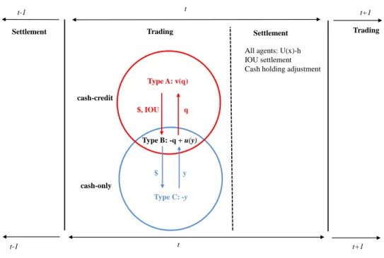
The economy is inhabited by three types – A, B and, C – of infinitely-lived agents, each of
measure one. In the settlement stage, all agents can consume or produce goodx. The utility
from consumption isU(x)withU0 >0andU00 <0. Producing one unit ofxrequires one unit
cash-credit
Type C: -y
cash-only
Trading
t t+1
Type B: -q + u(y)
Type A: v(q)
$, IOU q
All agents: U(x)-h IOU settlement Cash holding adjustment
Settlement
t-1
Trading Settlement
t t+1
t-1
$ y
Figure 2: Model Environment
of laborh, which incurs disutility of one. There existsx∗such thatU0(x∗) = 1. In the trading
stage, type A agents are active only in the cash-credit market, type C agents are active only
in the cash-only market, while type B agents participate in both markets. In the cash-credit
market, type A agents are buyers who wish to consume but cannot produce, and type B agents
are sellers who can produce but do not want to consume. Type A’s utility from consumingq
units of the good is v(q), with v0 > 0, v00 < 0, and v0(0) = ∞. The coefficient of relative
risk aversion, σq = −qv00(q)/v0(q), is less than1 everywhere. Type B’s cost of producingq
units of goods is q. There exists q∗ such that v0(q∗) = 1. In the cash-only market, type B
are buyers who cannot produce but would like to consume; their utility from consumption is
u(y), withu(0) = 0,u0 >0,u00<0, andu0(0) =∞. The coefficient of relative risk aversion,
σy =−yu00(y)/u0(y), is less than1everywhere. Type C agents are endowed with a productive
technology and can produceyunits of good at a cost ofy, but do not want to consume. There
existsy∗ such that u0(y∗) = 1. Assumeq∗ > y∗, or the cash-credit sector is larger than the
The period utility functions of the three types of agents are, respectively,
UA = v(qA) +U(x)−hA, (1)
UB = −qB+u(yB) +U(xB)−hB, (2)
UC = −yC +U(xC)−hC. (3)
Agents discount the next period’s utility by0< β <1.
The structure of the economy implies that there are potential gains from trade between
type A and type B agents in the cash-credit market, and between type B and type C agents
in the cash-only market. There are two payment instruments: cash (used interchangeably
with currency or money) and credit. A fraction, δ ∈ [0,1], of type A agents have access to
credit, type B agents accept both money and credit for sales of goodq,and typeCagents only
accept cash for payments. The stock of moneyM grows at a constant gross rate,γ > β. The
expansion (contraction) of the money supply is implemented as lump-sum transfers to (taxes
on) agents in the settlement stage in the amount of τ = (γ−1)M/3. Credit is extended in
the cash-credit market, and credit balances are settled in the next period’s settlement stage.10
Credit expansion is represented by a higher fraction of type A agents holding credit cards.
In each trading cycle, type A agents engage in the following activities. In the cash-credit
market, they trade with type B agents for goodqusing cash, credit, or both. In the settlement
stage, they adjust their money holdings and settle debt balances incurred in the previous
cash-credit market. Type B agents do the following. In the cash-cash-credit market, they sell good q
to type A agents, accepting either cash or credit. In the cash-only market, they use cash to
purchase goodyfrom type C agents. In the settlement stage, they adjust their money holdings
and settle credit balances incurred in the previous cash-credit market. Type C agents sell good
yto type B agents in the cash-only market, and spend money earned in the cash-only market
to purchase goodxin the settlement stage.
3.2
Equilibrium Characterization
In this subsection, we characterize the equilibrium allocation. The following notations are
used. The value functions in the trading stage and the settlement stage areV andW,
respec-tively. Let φ, φq,andφy denote the value of money in terms of x, q,andy,respectively. We
will use “ˆ” to denote variables in the next period. We will focus on symmetric-stationary
equilibria where the real variables, including the real cash balance, φM, are constant over
time. The equilibrium inflation rate is equal to the money growth rate γ, and the nominal
interest rate isi=γ/β−1>0.
3.2.1 Settlement Stage
Agents settle credit balances and adjust money holdings in the settlement stage. The value
function of an agent holdingm units of money andaunits of credit (a > 0, if the agent is a
creditor, anda <0, if the agent is a debtor) is
W(m, a) = max
x,h,mˆ U(x)−h+βV ( ˆm)
s.t. x+φmˆ =φ(m+τ) +a+h,
which can be rewritten as
W(m, a) = max
The first-order conditions are
x : U0(x) = 1orx=x∗,
ˆ
m : β∂Vj( ˆm)
∂mˆ ≤φ, “=” ifm >ˆ 0. (5)
The marginal value of money and credit balances in the settlement stage are, respectively,
∂W(m, a)
∂m =φ,and
∂W (m, a)
∂a = 1.
We measure the demand for cash as the real cash holdings at the beginning of the trading
stageφˆmˆ. A well-known result from the literature is that those who do not need to use cash
for payment (i.e., type A agents with access to credit and type C agents) will not take cash into
the trading stage ifi >0.
3.2.2 Trading Stage
First, we characterize the decisions for agents who do not take cash into the trading stage.
Type A agents with access to credit (use the subscript 1to denote variables associated with
these agents) buy goodqon credit and solve
max q1
v(q1) +W(0, pq1),
where pis the price of q in terms of goodx. In words, in the cash-credit market, the agent
buysq1units of goodqwith credit and promises to repaypq1units of goodxin the settlement
stage. The first-order condition forq1 is
Type C agents choose the production of good y (we omit the subscript knowing that in
equilibrium the production of type C is equal to the consumption of type B) to solve
max
y −y+W(y/φy,0).
The first-order condition is
y:φ=φy, (7)
which says that the relative price between goodyand goodxis one.
The value function of type A cash users (use the subscript 2 to denote variables associated
with these agents) is
V2(m2) = max
q2
v(q2) +W2(m2−q2/φq,0)
s.t. q2 ≤φqm2.
The agent buysq2units of goodqand pays for it withq2/φqunits of cash. Combine the value
functionsW andV to derive type A cash users’ maximization problem as
W2(m,0) = φm+τ +βW(0,0) (8)
+max
ˆ m2,q2
(
−φmˆ2+β
"
ˆ
φ mˆ2−
q2
ˆ
φq
!
+v(q2) +λ2( ˆφqmˆ −q2)
#) ,
where λ2 is the Lagrangian multiplier associated with the cash constraint. The first-order
conditions are11
ˆ
m2 : φ =β( ˆφ+λ2φˆq)⇒i=λ2
φq
φ ,
q2 : v0(q2) =
φ φq
+λ2 =
φ φq
(1 +i). (9)
11Note thatmˆ
As is standard in the literature, the cash constraint binds (i.e.,λ2 >0) ifi >0.
The value function for type B agents is
VB(mB) = max
qBm,qBc,y
−(qBm+qBc) +u(y) +W(mB+qBm/φq−y/φ,−pqBc)
s.t.y≤φ(mB+qBm/φq).
In words, a type B agent sellsqBm units of good in cash andqBcunits of good in credit in the
cash-credit market, and buysyunits of good in the cash-only market, which can be financed
by cash brought by the agent from the previous settlement stage and cash revenue in the
cash-credit market. Combine the value functions for type B agents to get
WB(m, a) = φ(m+τ) +a+βW(0,0) (10)
+ max
ˆ
mB,qBm,y
−φmˆB+β
ˆ
φmˆB+qφˆBq
−qBm−qBc+pqBc
+u(y)−y+λB
ˆ
φ( ˆmB+ qBmφˆq )−y
;
where λB is the Lagrangian multiplier associated with the cash constraint. The first-order
conditions are12
ˆ
mB : −φ+βφˆ(1 +λB)≤0orλB ≤i, “=” ifmˆB >0, (11)
y : u0(y) = 1 +λB,
qBm : 1 = (1 +λB)
φ φq
⇒u0(y)φ
φq
= 1, (12)
qBc : p= 1. (13)
Conditions (6) and (13) imply
q1 =q∗,
12Note thatq
and conditions (9) and (12) imply
u0(y)v0(q2) = 1 +i. (14)
The left-hand side of equation (14) captures the marginal benefit of holding cash (which can
be used in both the cash-credit and cash-only markets), and the right-hand side captures the
marginal cost.
To solve (q2, y), we need to look at type B agents’ cash flows. Type B agents receive cash
from type A cash users selling good q and spend cash on goody. Type A cash users’ cash
holding can be derived from their cash constraint q2 = ˆφqmˆ2, which implies z2 = ˆφmˆ2 =
ˆ
φq2/φˆq=q2φ/φq, or
z2 =
q2
u0(y). (15)
Type B agents therefore receive (1−δ)z2 = (1−δ)u0q(2y) units of cash by selling q in the
cash-credit market. If they receive enough cash from type A cash users to purchasey∗units of
good in the cash-only market, then they consume y∗ and hold zero cash. If the cash revenue
lies betweenyi and y∗, then type B agents continue to setzB to zero, and exhaust their cash
revenue for the purchase ofy. If the cash revenue is not enough to buyyi, which solves
u0(yi) = 1 +i,
type B agents’ consumption ofyand real cash holdingzBsatisfy
y =
y∗ if (1−δ) q2
u0(y) ≥y∗,
(1−δ) q2
u0(y) ifyi <(1−δ)u0q(2y) < y∗,
yi if (1−δ)u0q(2y) ≤yi.
(16)
zB =
0 if (1−δ)z2 ≥yi,
yi−(1−δ)z2 if (1−δ)z2 < yi.
(17)
Type B agents’ production ofqcan be derived from the market-clearing conditions
qBc = δq∗, (18)
qBm = (1−δ)q2. (19)
3.2.3 Equilibrium
The symmetric-stationary competitive equilibrium is defined as follows:
Definition 1 Given credit condition δ and nominal interest rate i, a symmetric-stationary equilibrium consists of
(i) a settlement stage allocationx=x∗ for all agents;
(ii) a trading stage allocationq1 =q∗,(q2, y)such that equations (14) and (16) hold, and
(qBm, qBc) given by equations (18) and (19); and
(iii) a distribution of cash holdings at the beginning of each periodz1 = zC = 0, and
(z2, zB)given by equations (15) and (17).
After solving the equilibrium allocation, we derive four quantities–the total money demand
value of cash transactions at points of salezT, and GDPY–all measured in units ofx.
z = (1−δ)z2+zB,
S = (1−δ)q2+δq ∗
u0(y) +y,
zT = (1−δ)z2+y=
(1−δ)q2
u0(y) +y,
Y = S+ 3x∗ = (1−δ)q2+δq ∗
u0(y) +y+ 3x ∗
.
From these quantities, we derive three ratios to characterize the demand for cash: the velocity
of cashυ(at points of sale), the share of cash transactions at points of saleθand the CIC/GDP
ratioρ
υ = zT
z , θ = zT
S , ρ= z Y .
4
Theoretical Implications
In this section, we explore the effect of credit expansion,δ, and the nominal interest rate,i, on
cash usage and demand. We will focus more on the effect of credit expansions for two reasons.
First, our model has very different implications from standard cash-credit models regarding
credit expansions. Second, the main mechanism that contributes to our model’s success in
capturing the cash paradox is the breakdown of the tight connection between cash usage and
demand in response to credit conditions. Regarding the effect of the interest rate, our model’s
prediction is similar to that from standard models. We conclude this section by discussing
the intuition about why our model is likely to be more successful than standard models in
i: 𝑖𝑖𝑖𝑖𝑖𝑖𝑖𝑖𝑖𝑖𝑖𝑖𝑖𝑖𝑖𝑖 𝑖𝑖𝑟𝑟𝑖𝑖𝑖𝑖
δ: 𝑟𝑟𝑎𝑎𝑎𝑎𝑖𝑖𝑖𝑖𝑖𝑖 𝑖𝑖𝑡𝑡 𝑎𝑎𝑖𝑖𝑖𝑖𝑐𝑐𝑖𝑖𝑖𝑖 1 − 𝑦𝑦∗/𝑞𝑞∗
𝛿𝛿2= 1 − 𝑦𝑦𝑖𝑖𝑢𝑢𝑢(𝑦𝑦𝑖𝑖)/𝑞𝑞∗
𝛿𝛿1= 1 − 𝑦𝑦∗/𝑞𝑞𝑖𝑖
𝑖𝑖: 𝑞𝑞𝑖𝑖= 𝑦𝑦∗
o
Regime I
Regime II
Regime III
𝑧𝑧𝐴𝐴> 0
𝑧𝑧𝐵𝐵= 0
𝑦𝑦 = 𝑦𝑦∗
𝑞𝑞 = 𝑞𝑞𝑖𝑖
𝑧𝑧𝐴𝐴> 0
𝑧𝑧𝐵𝐵= 0
𝑦𝑦𝑖𝑖< 𝑦𝑦 < 𝑦𝑦∗
𝑞𝑞𝑖𝑖< 𝑞𝑞 < 𝑞𝑞∗
𝑧𝑧𝐴𝐴> 0
𝑧𝑧𝐵𝐵> 0
𝑦𝑦 = 𝑦𝑦𝑖𝑖
𝑞𝑞 = 𝑞𝑞∗
Figure 3: Regimes
4.1
Effects of Credit Expansion
As credit expands or asδincreases from 0 to 1, the economy will be in one of three regimes,
distinguished by whether or not type B agents consumey∗in the cash-only market and whether
or not they take cash into the trading stage. The threshold values ofδthat separate these three
regimes depend on the nominal interest rate. In Figure 3, we mark the border of each regime
in the(δ, i)space.
4.1.1 Regime I: Low Credit Regime
In regime I, type B agents receive enough cash revenue in the cash-credit market to purchase
y∗units of consumption in the cash-only market(y=y∗), and do not take cash into the trading
is given by
z2 = qi,
zB = 0,
z = zA = (1−δ)z2 = (1−δ)qi,
zT = (1−δ)qi+y∗.
If y∗ < qi, then the economy starts in regime I when δ = 0 and remains in this regime if
(1−δ)qi ≥y∗, or
δ≤δ1 ≡1−
y∗ qi
.
Ify∗ > qi, then the economy will not experience regime I and will be in regime II whenδ = 0.
The velocity of cash is
υ = zT
z = 1 +
y∗
(1−δ)qi
.
The share of cash transactions at points of sale is
θ = zT
S =
(1−δ)qi+y∗
(1−δ)qi+y∗+δq∗
.
The CIC/GDP ratio is
ρ= z
Y =
(1−δ)qi
(1−δ)qi+y∗+δq∗+ 3x∗
.
Proposition 1 The Effects of δ in regime I: dq1/dδ = dq2/dδ = dy/dδ = 0, dzT/dδ =
dz/dδ <0,dυ/dδ >0,dθ/dδ <0,anddρ/dδ <0.
Proof.See Appendix A.
In regime I, the allocation(q1, q2, y)is invariant to δ. Type B agents receive enough cash
from type A cash users to purchase y∗ and their demand for cash is zero. As more type A
A agents (which is also the total demand for cash), and the CIC/GDP ratio all decrease. By
construction, the velocity of cash at points of sale is between one and two. After type B agents
receive cash from their customers, a fixed amount (y∗) of it is spent in the cash-only sector
and this part of cash has a higher velocity of two. As type B agents receive less cash from
their customers in the cash-credit sector, the fraction of cash that travels twice in the trading
stage increases, resulting in a higher velocity.
4.1.2 Regime II: Intermediate Credit Regime
In regime II, type B agents do not have enough cash revenue in the cash-credit market to
support consumption of y∗ in the cash-only market. However, as long asy > yi, the benefit
of taking cash into the trading stage, u0(y), is lower than the cost, 1 +i, and type B agents’
cash demand is zero. They simply spend all the cash received from the cash-credit market to
purchaseyon the cash-only market. As a result,q2 andyjointly solve (14) and
y= (1−δ)q2
u0(y) ,
which follows from (15) and (16). Money demand is given by
zB = 0,
z2 =
q2
u0(y) =
y
1−δ,
z = zA= (1−δ)z2 =y,
zT =
(1−δ)q2
u0(y) +y= 2y.
This regime occurs when
whereδ2 solvesyi = (1−δ)q∗/u0(yi), or
δ2 ≡1−
yiu0(yi)
q∗ .
Note thatd[yu0(y)]/dy =u0(y) +yu00(y)>0under the assumptionσy =−yu00(y)/u0(y)<1.
Since yi < y∗, we have yiu0(yi) < y∗u0(y∗) = y∗ < q∗ and δ2 > 0, and the economy will
experience regime II for sure asδincreases from0.
In regime II, the cash taken by type A cash users into the trading stage is used twice: once
in the cash-credit market and once in the cash-only market. The velocity of cash is therefore
υ = zT
z = 2.
The share of cash transactions at points of sale is
θ = zT
S =
2y
2y+δuq0(∗y)
,
and the CIC/GDP ratio is
ρ= z
Y =
y
2y+ uδq0(∗y)+ 3x∗
.
In regime II, the effects of credit expansions is described in the following proposition.
Proposition 2 The effects ofδin regime II:dq1/dδ = 0,dq2/dδ > 0,dy/dδ < 0, dzT/dδ = 2dz/dδ <0,dυ/dδ= 0,dθ/dδ <0,anddρ/dδ <0.
Proof.See Appendix A.
In regime II, type B agents still choose not to take any cash to the trading stage. As the
fraction of type A credit users increases, type A agents’ (and therefore, the total) cash demand
CIC/GDP ratio continues to decrease.13
4.1.3 Regime III: High Credit Regime
As the fraction of credit card users continues to increase beyond δ2, type B agents do not
receive enough cash to purchaseyi. In this situation, type B agents start to accumulate some
cash to make up for the decreasing cash revenue in the cash-credit market (see equation 17).
The economy enters into regime III. In this regime, the marginal benefit of consuming y is
higher than that in Regime II and equal to 1 + i, the marginal cost of acquiring money in
the settlement stage. The cash-only market output is y = yi. Since type B agents are cash
constrained in the only market, they are willing to pay more to acquire cash in the
cash-credit market compared to the previous regimes. This leads toq2 =q∗; i.e., type A cash users
can afford the first-best consumption.14 The money demand is given by
z2 =
q∗ u0(y) =
q∗
1 +i,
zA = (1−δ)z2,
zB = yi−(1−δ)z2 =yi−(1−δ)
q∗
1 +i,
z = zB+zA =yi,
zT =
(1−δ)q∗
u0(y) +yi = (1−δ)
q∗
1 +i +yi.
13Gu et al. (2016) recently demonstrate that the increase in credit limits is neutral in a wide range of environ-ments. Our model provides a counter example. In our Bank of Canada Staff Working Paper version, Jiang and Shao (2014), we capture credit expansions along the intensive margin as increasing credit limits as in Gu et al. (2016), and find that when the economy is in regime II, a higher credit limit is not neutral: it expands cash-credit activities (q) and shrinks cash-only activities (y).
The velocity of cash, the share of cash transactions at points of sale and the CIC/GDP ratio
are, respectively,
υ = zT
z = 1 +
(1−δ)q∗
(1 +i)yi
, (20)
θ = zT
S =
(1−δ)1+q∗i +yi q∗
1+i +yi
, and (21)
ρ = z
Y =
yi q∗
1+i +yi+ 3x
∗. (22)
The effect of credit expansion in this regime is described in the proposition below. (The
proof is trivial and therefore omitted.)
Proposition 3 The effects ofδin regime III:dq1 =dq2/dδ=dy/dδ = 0,dzT/dδ =−q∗/(1+
i) <0, dz/dδ = 0, dυ/dδ =−q∗/[(1 +i)yi)]< 0,dθ/dδ = −q∗/[q∗ + (1 +i)yi] < 0, and
dρ/dδ = 0.
Once the economy enters into regime III, a further credit expansion reduces the value of
cash transactions, but the total money demand becomes flat. The reduction in type A agents’
money demand is exactly offset by the rise in type B agents’ money demand.
Figure 4 summarizes the effect of credit expansions on allocation(q2, y), money demand
(zA, zB), cash velocity υ, the share of cash transactionsθ, and CIC/GDPρ as the fraction of
type A agents with access to credit increases from0to1.
While a standard cash-credit model predicts continuous and synchronized falls in cash
usage and demand in response to credit expansions (see Appendix D), our model suggests
that this trend stops as credit expands beyond a certain level. In particular, onceδreachesδ2,
agents change their cash management practices and further credit expansions induce a
redistri-bution of cash demand. Buyers in the cash-credit sector hold less cash to spend in that sector,
while sellers in that sector acquire more cash in advance to make up for the shortfall of cash
δl 1
𝒒𝒒𝒊𝒊
𝒒𝒒∗
𝒚𝒚𝒊𝒊
𝒚𝒚∗
Figure 3: Effect of credit expansion
0 0
0 0
1
v
0
θ
0
2
δ2 δ
δl δ2 1 δ
δl δ2 1 δ δl δ2 1 δ
δl δ2 1 δ
δl δ2 1 δ
𝒒𝒒𝟐𝟐
y
𝒛𝒛𝑨𝑨; 𝒛𝒛𝑩𝑩 ρ
Figure 4: The effects of credit expansion
cash remains constant despite reduced cash usage. Compared with cash acquired by buyers,
which is used in both sectors, cash acquired by sellers has a lower velocity because it is used
exclusively in the cash-only sector. As a result, the redistribution of cash demand reduces the
overall velocity of cash.15
4.2
Effects of Interest Rate
Besides the credit access condition, the interest rate is another important parameter that affects
cash usage and demand. Our model’s prediction on the effect of the interest rate is similar to
that of standard cash-credit models, which we summarize in the following proposition.
Proposition 4 The effects ofi: dq1/di= 0;dq2/di <0in regimes I and II, and= 0in regime III;dy/di = 0in regime I, and<0in regimes II and III;dz/di < 0,dρ/di < 0,dθ/di < 0;
dυ/di >0in regimes I and III, and= 0in regime II.
Proof.See Appendix A.
As the interest rate rises, the cost of holding cash increases. Consumption financed by
cash, q2 and y, decreases (unless q2 = q∗ or y = y∗). Cash usage and cash demand both
decrease in response to higher interest rates.
In terms of velocity, our model provides a theory about the positive correlation between
the variable and inflation, the so-called hot potato effect of inflation. In particular, inflation
affects velocity by changing the fraction of money that sits idle in either the cash-only or the
cash-credit market.
The specification of our model implies that cash velocity lies between one and two. In
regime II, all cash is used in both markets so the velocity is fixed at the upper bound of two. In
regimes I and III, a fraction of cash sits idle in one of the two markets, and this fraction changes
in response to inflation. In regime I, type B agents use part of their cash revenues received
from type A cash users in the cash-credit market to finance a fixed level of purchase (y∗) in the
cash-only market, with the surplus cash sitting idle in the second market. As inflation rises,
type A cash users acquire less cash, which means that type B agents receive less cash and
have less idle balances in the cash-only market. As a result, velocity increases. In regime III,
both type A and B agents acquire money balances in advance. The amount acquired by type
B agents is spent only in the cash-only market and sits idle in the cash-credit market. The
amount acquired by type A cash users is spent in both markets and has a higher velocity. Both
types acquire less cash in response to higher inflation. However, type B agents reduce their
cash holdings more than type A cash users, causing the fraction of cash that sits idle in the
cash-credit market to fall. Consequently, the overall velocity of cash increases.16
Ro-5
Capturing the Cash Paradox
In the previous section, we develop a model that adds two new features into a standard
cash-credit model: different substitutability between cash and cash-credit across sectors, and cash flows
between the two sectors. In this section, we carry out a series of calibration exercises to
highlight the roles played by these two modelling features. First, we calibrate a standard
cash-credit model with a single sector. We then calibrate a model with two segregated sectors
that feature different substitutability between cash and credit (and label it the no-cash-flow or
“NCF” model) to identify the role played by this modelling feature. Finally, we calibrate the
full model with both modelling features to discuss the importance of the cash-flow channel.
For the calibration, we use constant-relative-risk-aversion (CRRA) utility functions
v(q) = sq
1−α
1−α andu(y) =
y1−η
1−η.
The curvature parameters α and η indicate the demand elasticity of the interest rate for the
cash users when they are liquidity constrained.17 In our calibration, we setα = ηso that the
two markets have the same interest rate elasticity.18 According to our theory, we setα∈(0,1)
in the full model, but do not restrict it to be less than 1 for the standard model and the NCF
model. The scaling parameter s >0captures the size of the cash-credit sector relative to the
cash-only sector.
Our calibration strategy is to use the time series of the credit access rate(δ)and the nominal
interest rate (i), and fit model parameters (α, s, x∗) to match the time series of CIC/GDP,ρ.
More specifically, for each parameter triplet (α, s, x∗), we plug(α, s, x∗)and (δt, it)into the
cheteau, 2005; Faig and Jerez, 2006; Ennis, 2008 and 2009; Liu et al., 2011; Nosal 2011; Dong and Jiang, 2013; and Hu et al., 2017). All these models feature a precautionary demand for money, while we identify a different mechanism that does not rely on the precautionary motive.
17When the cash users are liquidity constrained, the demand for type A cash user isq
iand the demand for type B cash user isyi. The demand elasticity is thenα(1+i)i andη(1+i)i , respectively.
expression forρto calculate the model’s prediction of CIC/GDP in periodt,ρˆt(δt, it|α, s, x∗).
We then do a grid search in the(α, s, x∗)space to minimize the sum of squared errors of the
predicted series of CIC/GDP from its actual path:
( ˆα,s,ˆ xˆ∗) = arg min
α,s,x∗
X
t
[ ˆρt(δt, it|α, s, x∗)−ρt] 2
.
In the case of the standard model, there is only one sector where cash and credit are perfect
substitutes (whereq is traded) and we sets = 1and grid search over the (α, x∗) space. Our
calibration strategy is in the same spirit as that in Lagos and Wright (2005) and follows the
tra-dition of Lucas (2000). The difference is that instead of fitting the model parameters to match
the money demand equation ρ(i), we fit the parameters to match the time series of money
demand over the sample period,ρt. After we acquire the model parameters, we calculate the
imputed series for cash usage and demand,θˆandρˆ.
We calibrate the models to the cases of four countries, Australia, Canada, the United
King-dom and the United States. The sample period spans from 1960 to 2014.19 We start from 1960
because it was not until 1958 that major banks issued credit cards. We use the (annualized)
short-term safe corporate bond rate to measure the nominal interest rate.20 To the best of our
knowledge, continuous time series data on the credit access rate are unavailable, so we have to
resort to various surveys to construct it. In each country over the sample period from 1960 to
2014, infrequent surveys that provide information on the fraction of households holding credit
cards were conducted. To fill in the missing years, we fit a polynomial function across the
available observations, together with an initial pointδ1960 = 0, to impute the series ofδfor the
entire sample period.
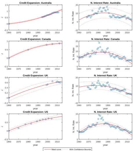
Figure 5 shows the trend in credit expansions and nominal interest rates in the data. There
19The sample period for Australia and the United Kingdom starts at 1968 and 1973, respectively, because the nominal interest rate data on these countries start from those years.
year
1960 1970 1980 1990 2000 2010
/
-0.5 0 0.5 1
1.5 Credit Expansion: Australia
fitted curve 95% Confidence Bounds
year
1960 1970 1980 1990 2000 2010
N. Int. Rate
-10 0 10
20 N. Interest Rate: Australia
year
1960 1970 1980 1990 2000 2010
/
-0.5 0 0.5
1 Credit Expansion: Canada
year
1960 1970 1980 1990 2000 2010
N. Int. Rate
-5 0 5 10 15
20 N. Interest Rate: Canada
year
1960 1970 1980 1990 2000 2010
/ -0.2 0 0.2 0.4 0.6
0.8 Credit Expansion: UK
year
1960 1970 1980 1990 2000 2010
N. Int. Rate
-10 0 10
20 N. Interest Rate: UK
year
1960 1970 1980 1990 2000 2010
/
-0.5 0 0.5
1 Credit Expansion: US
year
1960 1970 1980 1990 2000 2010
N. Int. Rate
0 5 10
15 N. Interest Rate: US
Figure 5: Time paths of credit access rate and nominal interest rate
is a clear upward trend forδdue to financial innovations. The nominal interest rate appears to
be hump-shaped, rising until the 1980s and declining afterwards. While calculatingρˆ, we use
the imputed series ofδand the actual series ofi(the trend curve foriis plotted for reference).
The upper panel from Table 1 summarizes the calibrated parameter values (α,ˆ ˆs,xˆ∗) for
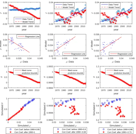
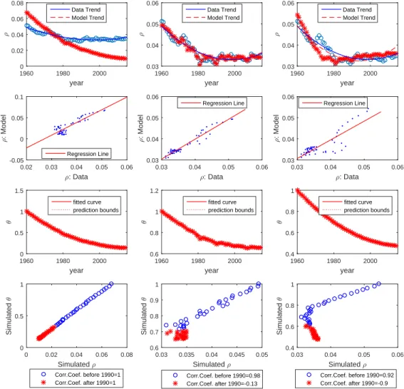
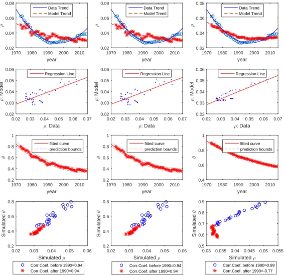
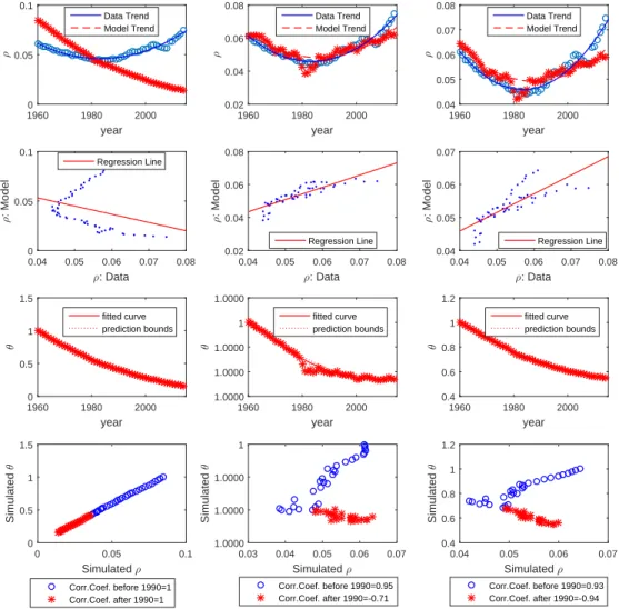
each country for each of the three models. Figures 6 to 9 plots the three models’ prediction
on ρ and θ. Each figure represents one country and has twelve panels. The left column of
actual and predicted series ofρalong with their corresponding (polynomial) time trends. The
second graph scatter plots actual versus predictedρ(together with a regression line). The third
panel plots the predicted series ofθand its trend. The fourth panel scatter plotsρversusθ; the
circles represent data before 1990, and the stars represent data from 1990.
The lower panel of Table 1 provides two statistics to measure the performance of the model
in capturing the long-run trend in cash demand. The first is the normalized root-mean-square
error (NRMSE) for the predicted path ofρ:
N RM SE =
q
1 N
P
t[ ˆρt(δt, it|α,ˆ ˆs,xˆ∗)−ρt] 2
¯
ρ ,
whereN is the sample size, andρ¯= 1
N
P
tρt is the average CIC/GDP in the sample period.
The second is the correlation between the predicted and actual series of ρ. The third and
fourth rows show the model’s prediction on the correlation between θ and ρ for two
subpe-riods, before 1990 and thereafter, respectively (note that the data suggest that the correlation
is positive before 1990 and negative after 1990).21 The last row reports the (NCF and full)
model’s implied relative size of the cash-credit sector, measured byq∗ (y∗is normalized to1).
Finally, Table 2 reports the share of cash transactions (calculated as the value of cash
transactions over the sum of cash and credit transactions) based on recent payment surveys:
the consumer payment diary surveys conducted in 2009 (Canada), 2010 (Australia), and 2012
(US), and the British Retail Consortium Payment Survey in 2016, which samples merchants.
For comparison, we calculate the average value ofθˆfrom 2005 to 2014 (which are the last 10
years for our calibration exercises) implied by each model.
21We also calculate the correlation betweenρˆandθˆ, splitting the sample at different time points between 1980
year
1970 1980 1990 2000 2010
; 0.03 0.035 0.04 Data Trend Model Trend
;: Data
0.03 0.035 0.04 0.045
; : Model 0.03 0.032 0.034 0.036 0.038 Regression Line year
1970 1980 1990 2000 2010
3 0.4 0.6 0.8 1 1.2 fitted curve prediction bounds
Simulated ;
0.03 0.032 0.034 0.036 0.038
Simulated 3 0.4 0.6 0.8 1
Corr.Coef. before 1990=0.88 Corr.Coef. after 1990=-0.73
year
1970 1980 1990 2000 2010
; -0.02 0 0.02 0.04 0.06 Data Trend Model Trend
;: Data
0.03 0.035 0.04 0.045
; : Model -0.02 0 0.02 0.04 0.06 Regression Line year
1970 1980 1990 2000 2010
3 -0.5 0 0.5 1 1.5 fitted curve prediction bounds
Simulated ;
0 0.02 0.04 0.06
Simulated
3
0 0.5 1
Corr.Coef. before 1990=0.99 Corr.Coef. after 1990=1
year
1970 1980 1990 2000 2010
; 0.03 0.035 0.04 Data Trend Model Trend
;: Data
0.03 0.035 0.04 0.045
; : Model 0.03 0.032 0.034 0.036 0.038 Regression Line year
1970 1980 1990 2000 2010
3 0.9994 0.9996 0.9998 1 1.0002 fitted curve prediction bounds
Simulated ;
0.03 0.032 0.034 0.036 0.038
Simulated 3 0.9994 0.9996 0.9998 1
Corr.Coef. before 1990=0.9 Corr.Coef. after 1990=-0.69
Figure 6: Model predictions–Australia
year
1960 1980 2000
; 0 0.02 0.04 0.06 0.08 Data Trend Model Trend
;: Data
0.02 0.03 0.04 0.05 0.06
; : Model -0.05 0 0.05 0.1 Regression Line year
1960 1980 2000
3 0 0.5 1 1.5 fitted curve prediction bounds
Simulated ;
0 0.02 0.04 0.06 0.08
Simulated
3
0 0.5 1
Corr.Coef. before 1990=1 Corr.Coef. after 1990=1
year
1960 1980 2000
; 0.03 0.04 0.05 0.06 Data Trend Model Trend
;: Data
0.03 0.04 0.05 0.06
; : Model 0.03 0.04 0.05 0.06 Regression Line year
1960 1980 2000
3 0.4 0.6 0.8 1 fitted curve prediction bounds
Simulated ;
0.03 0.04 0.05 0.06
Simulated 3 0.4 0.6 0.8 1
Corr.Coef. before 1990=0.92 Corr.Coef. after 1990=-0.9
year
1960 1980 2000
; 0.03 0.04 0.05 0.06 Data Trend Model Trend
;: Data
0.03 0.04 0.05 0.06
; : Model 0.03 0.04 0.05 0.06 Regression Line year
1960 1980 2000
3 0.6 0.8 1 1.2 fitted curve prediction bounds
Simulated ;
0.03 0.035 0.04 0.045 0.05
Simulated 3 0.6 0.7 0.8 0.9 1
Corr.Coef. before 1990=0.98 Corr.Coef. after 1990=-0.13
Figure 7: Model predictions–Canada
year
1970 1980 1990 2000 2010
; 0.02 0.04 0.06 0.08 Data Trend Model Trend
;: Data
0.02 0.03 0.04 0.05 0.06 0.07
; : Model 0.02 0.03 0.04 0.05 0.06 Regression Line year
1970 1980 1990 2000 2010
3 0.2 0.4 0.6 0.8 1 fitted curve prediction bounds
Simulated ;
0.02 0.03 0.04 0.05 0.06
Simulated 3 0.2 0.4 0.6 0.8
Corr.Coef. before 1990=0.94 Corr.Coef. after 1990=0.94
year
1970 1980 1990 2000 2010
; 0.02 0.04 0.06 0.08 Data Trend Model Trend
;: Data
0.02 0.03 0.04 0.05 0.06 0.07
; : Model 0.02 0.03 0.04 0.05 0.06 Regression Line year
1970 1980 1990 2000 2010
3 0.4 0.6 0.8 1 fitted curve prediction bounds
Simulated ;
0.03 0.035 0.04 0.045 0.05 0.055
Simulated 3 0.5 0.6 0.7 0.8 0.9
Corr.Coef. before 1990=0.99 Corr.Coef. after 1990=-0.77
Figure 8: Model predictions–UK
year
1960 1980 2000
; 0.02 0.04 0.06 0.08 Data Trend Model Trend
;: Data
0.04 0.05 0.06 0.07 0.08
; : Model 0.02 0.04 0.06 0.08 Regression Line year
1960 1980 2000
3 1.0000 1.0000 1.0000 1 1.0000 fitted curve prediction bounds
Simulated ; 0.03 0.04 0.05 0.06 0.07
Simulated 3 1.0000 1.0000 1.0000 1
Corr.Coef. before 1990=0.95 Corr.Coef. after 1990=-0.71
year
1960 1980 2000
; 0 0.05 0.1 Data Trend Model Trend
;: Data
0.04 0.05 0.06 0.07 0.08
; : Model 0 0.05 0.1 Regression Line year
1960 1980 2000
3 0 0.5 1 1.5 fitted curve prediction bounds
Simulated ;
0 0.05 0.1
Simulated 3 0 0.5 1 1.5
Corr.Coef. before 1990=1 Corr.Coef. after 1990=1
year
1960 1980 2000
; 0.04 0.05 0.06 0.07 0.08 Data Trend Model Trend
;: Data
0.04 0.05 0.06 0.07 0.08
; : Model 0.04 0.05 0.06 0.07 Regression Line year
1960 1980 2000
3 0.4 0.6 0.8 1 1.2 fitted curve prediction bounds
Simulated ;
0.04 0.05 0.06 0.07
Simulated 3 0.4 0.6 0.8 1 1.2
Corr.Coef. before 1990=0.93 Corr.Coef. after 1990=-0.94
Figure 9: Model predictions–US
Table 2: Cash shares relative to credit,θ
Australia Canada UK US
Data 0.64(1) 0.36(1) 0.52(2) 0.45(1)
Standard(3) 0.06 0.15 0.37 0.19
NCF(3) 1.00 0.66 0.39 1.00
Full(3) 0.52 0.49 0.60 0.56
Notes: (1) Data are based on payment diary surveys conducted in 2009 (Canada), 2010 (Aus-tralia), and 2012 (US); source: Bagnall et al. (2016). (2) The data on UK are from the 2016 British Retail Consortium Payment Survey. (3) The model’s cash share is the average value from 2005 to 2014.
5.1
The Standard Model
In the standard model, cash usage and demand are characterized by (see Appendix D for the
derivation)
θ = (1−δ)qi
(1−δ)qi+δq∗
, (23)
ρ = (1−δ)qi
(1−δ)qi+δq∗+ 2x∗
. (24)
Bothθandρdecrease withδandi. In earlier decades, the effect of the two parameters works
in the same direction (δand iboth increase). In more recent decades, however, the effect of
the two parameters works against each other (δcontinues to rise whileistarts to decrease). To
capture the cash paradox, the effect ofδ must dominate to capture the time trend inθ, while
the opposite is required to capture the trend in ρ. Although in theory it is still possible that
cash usage and demand can diverge from each other, these conflicted requirements imply that
it is difficult for standard cash-credit models to capture the cash paradox.
As shown in Table 1, the standard model is unable to resolve the cash paradox. Although
it generates continuously declining cash usage (θ), which is consistent with data, the predicted
40.7% for Canada, 17.8% for the United Kingdom, and 49.5% for the United States. The
correlation betweenρandρˆis even negative for Australia and the United States. In addition,
the standard model fails to account for the diverging trend in cash usage and demand in the
more recent decades: the correlation between θˆand ρˆis positive for all four countries after
1990.
5.2
The NCF Model
In the NCF model, cash usage and demand are given by (see Appendix E for the derivation):
θ = (1−δ)qi+yi
(1−δ)qi+δq∗+yi
,
ρ = (1−δ)qi +yi
(1−δ)qi+δq∗+yi+ 4x∗
.
Compared with the standard model, the NCF model is more flexible and allows the relative
effect of credit accessibility and the interest rate to differ in these two sectors. Note that δ
affects only the cash-credit sector, andiaffects both sectors. A smallerstends to increase the
relative importance ofi.
The NCF model’s performance is similar to the standard model for the United Kingdom
(and fails to capture the cash paradox). The model performs very well in terms of capturing
the cash demand series in the other three countries: the NRMSE forρshrinks substantially to
4.5% in Australia, 3.4% in Canada, and 7.0% in the United States.
The mechanism through which the NCF model captures the trend in money demand is as
follows. Note that the imputed value of s, which captures the size of the cash-credit sector
relative to the cash-only sector, is very small for Australia (at 0.003) and the United States (at
0.137). Together with the power of the utility functionα, it implies thatq∗is very close to zero
to the cash-only sector, which is hard to justify for advanced economies. For cash demand, a
negligible cash-credit sector means that the demand for cash is almost entirely driven by the
demand in the cash-only sector, which is shielded against credit expansions and has increased
in response to lower interest rates in the past two to three decades. However, the success
story for cash demand comes at a cost: the implied relative size of the cash-credit sector is
unreasonably low. In addition, although the model predicts that θ decreases over time, the
magnitude of changes is infinitesimal and the share of cash transactions has remained close to
1in the last six decades.
The NCF model does reasonably well for Canada. Although the cash-credit sector is still
smaller than the cash-only sector (q∗ = 0.648), the difference is not as extreme as in Australia
and the United States. The imputedθ averages at 66%from 2005 and 2014 (the survey data
suggest that the share of cash transactions is about 36% in 2009 in Canada).
5.3
The Full Model
The full model, which incorporates the cash-flow channel, generates continuous and
substan-tial declines in cash usage (θ) as suggested by the data. It also captures the time trend of
cash demand well. The NRMSE is small, ranging from 4.5% (in Australia) to 14.4% (in the
United Kingdom). It predicts that, despite continuing drops in cash usage, cash demand
de-clines only in earlier years, but stabilizes or increases in the more recent two or three decades,
successfully capturing the cash paradox. In all four countries, the correlation between cash
usage and demand is positive before 1990, but becomes negative afterwards. According to the
calibration, the cash-credit sector is larger than the cash-only sector in all four countries, and
the implied cash share is much more reasonable: the average cash share in 2005-2014 ranges
from 49% (in Canada) to 60% (in the United Kingdom).