BAYESIAN ANALYSIS OF ULTRA-HIGH DIMENSIONAL NEUROIMAGING DATA
Michelle Ferreira Miranda
A dissertation submitted to the faculty at the University of North Carolina at Chapel Hill in partial fulfillment of the requirements for the degree of Doctor of Philosophy in the
Department of Statistics and Operations Research.
Chapel Hill 2014
Approved by: Joseph G. Ibrahim Hongtu Zhu Yufeng Liu
©2014
ABSTRACT
Michelle Ferreira Miranda: Bayesian analysis of ultra-high dimensional neuroimaging data (Under the direction of Joseph G. Ibrahim and Hongtu Zhu)
Medical imaging technologies have been generating extremely complex data sets. This dissertation makes further contributions to the development of statistical tools motivated by modern biomedical challenges. Specifically we develop methods to characterize varying associations between ultra-high dimensional imaging data and low-dimensional clinical outcomes.
The first part of this dissertation is motivated by the major limitations faced by traditional voxel-wise models, where voxels are commonly treated as independent units, and the assumption of Gaussian distribution of the neuroimaging measurements is usually flawed. We develop a class of hierarchical spatial transformation models to model the spatially varying associations between imaging measurements in a three-dimensional (3D) volume (or 2D surface) and a set of covariates. The proposed approach include a spatially varying Box-Cox transformation model and a Gaussian Markov random field model.
ACKNOWLEDGEMENTS
I would like to first thank my advisors Hongtu Zhu and Joseph Ibrahim. Joseph, thank you for teaching me Bayesian statistics in such a beautiful and inspiring way. Hongtu, thank you for the lessons in imaging analysis and for your determination in making things work. I am always amazed by your ability to manage your students, knowing in details what we are doing, even though we are so many. Both of you contributed tremendously to my path as a researcher and I am forever grateful for that.
Many others contributed to this achievement in a direct or indirect way:
• Susan and Diana, for the many hours spent at the Looking Glass studying for the comps;
• Eric and Dominik, for being my very first friends, for the weekly beer nights, for the dancing nights;
• Sean, for making me laugh with your funny stories;
• The quartet on Main street, Susan, Diana, Sean and Eric for the trips, countless board games and dinner nights. I am grateful for having such amazing friends!!!
• My friend and first roommate Fernanda, who taught me so much about kindness and became part of my family;
• Julien and Marc, for the weekly wine bar nights;
• My salsa friends Derek and Chris, who helped me to be sane during this last couple of years;
• My Brazilian friends, who made my first months here so enjoyable;
• My family, who always sent me their love in prayers and positive thinking; • Bruno, for always being the one I could count for help;
• My sister Izabela, who is always ready to give me the right advice;
• My friends Arianna, Bia, Felipo, kelly e Taty who have been my rock for decades.
Thank you very much to my best friend Susan Wei, for helping me with my writing, listening to my frustrations and excitements, and for always being there. You always inspired me and pushed me forward!!
Thank you Sepehr, for being my English teacher, my proof reader and for helping me to cross the ending line. Your support and companionship were essential during my final steps.
PREFACE
TABLE OF CONTENTS
LIST OF TABLES . . . x
LIST OF FIGURES . . . .xi
CHAPTER 1: INTRODUCTION . . . 1
1.1 Voxel-wise models . . . 1
1.2 Low-rank regression models . . . 2
1.3 Outline of Thesis . . . 3
CHAPTER 2: BAYESIAN SPATIAL TRANSFORMATION MODELS . . . 4
2.1 Introduction . . . 4
2.2 Model . . . 6
2.2.1 Model Description . . . 6
2.2.2 Priors . . . 9
2.2.3 Posterior Computation . . . 9
2.3 Simulation Study . . . .11
2.4 Application to the ADHD dataset . . . .15
2.5 Discussion . . . .21
CHAPTER 3: TENSOR PARTITION REGRESSION MODELS . . . .22
3.1 Introduction . . . .22
3.2 Methodology . . . .25
3.2.1 Preliminaries . . . .25
3.2.2 Tensor Partition Regression Models . . . .26
3.2.3 Prior Distributions . . . .28
3.3 Simulation Study . . . .32
3.3.1 Bayesian tensor decomposition . . . .32
3.3.2 A 2-dimensional image example . . . .33
3.3.3 A 3D image example . . . .38
3.4 Real data analysis . . . .40
3.5 Discussion . . . .44
CHAPTER 4: SPARSE PARTITION FACTOR MODELS . . . .45
4.1 Introduction . . . .45
4.2 Model . . . .47
4.2.1 Model Description . . . .47
4.2.2 Prior distributions . . . .49
4.2.3 Posterior Inference . . . .49
4.3 Simulation Study . . . .53
4.4 Application to the ADHD data set . . . .56
4.5 Discussion . . . .60
CHAPTER 5: FUTURE WORK . . . .61
5.0.1 Spatial transformation models . . . .61
5.0.2 Low-rank models . . . .61
APPENDIX A: CHAPTER 2 SUPPLEMENTARY MATERIAL . . . .62
A.1 Full conditionals derivations . . . .62
A.2 Sensitivity Analysis . . . .63
A.3 Examining the effects of differentHkon the parameter estimates ofβ . . . .67
A.4 Additional results . . . .70
A.5 How to run BSTM? . . . .72
A.5.1 Simulation code . . . .72
LIST OF TABLES
3.1 Root mean squared error for 3 different image modalities. The Bayesian decomposition outperforms the alternating least squares in each scenario. There is a smaller error measurement with an increase of the rankR. . . 34 4.1 Deviance information criteria for the partition modelsNs = 8andNs= 18
and the non-partition model. Based on the criteria, the models withNs= 18 are preferred. The symbol ** indicates the models that did not converge. . . 56 4.2 Deviance information criteria for the partition modelsNs = 8andNs = 24
and the non-partition model. Based on the criteria, the partition models are preferred. . . 57 A.1 Sensitivity analysis forλindicating the percentages of voxels, whose Geweke
LIST OF FIGURES
2.1 Simulation results: the trueΛ = {λd, d ∈ D} pattern in the left panel and the estimated pattern in the right panel. Estimated image is smoother compared with the true image due to the nature of the uniform distribution assumeda priori. This figure appears in color
in the electronic version of this article. . . 13 2.2 Simulation results on comparison of STM, GMRF with no
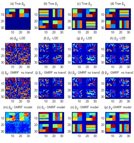
transfor-mation, and the voxel-wise linear model. Panels (a)-(d) represent the pattern ofβused to generate the images; panels (e)-(h) repre-sent the estimatedβobtained from the least squares estimator in Matlab; panels (i)-(l) represent the posterior mean ofβobtained by fitting a GMRF model with no transformation; and panels (m)-(p) are the posterior mean ofβobtained from our STM. The inclusion of the transformation parameter substantially improves the estima-tion of the true underlying pattern. This figure appears in color in
the electronic version of this article. . . 14 2.3 Trace plots forβ,τσ andλfor a randomly generated voxel. The
results are for a 1000 iterations of the MCMC algorithm and a burn-in sample of 50. The trace plots indicate a fast convergence of the algorithm, confirming its efficiency and good mixing properties.
This figure appears in color in the electronic version of this article. . . 15 2.4 White matter RAVENS map for two randomly selected children
from the ADHD study. The image from subject b shows a higher brightness inside the square, reflecting the fact that for the brain of subject b, relatively more white matter was forced to fit the same template (panel (c)) at that particular region. This figure appears in
color in the electronic version of this article. . . 17 2.5 ADHD data analysis results: normal probability plots of sixteen
random voxels revealing that the imaging measurements extracted from the RAVENS map deviate from the Gaussian distribution.
2.6 ADHD data analysis results: selected slices showing the estimated
ˆ
Λfor the imaging data obtained from the white matter RAVENS map. Panels (a)-(c) represent respectively, a coronal, sagittal and axial view of selected slices of the brain. The line indicates where the coronal and sagittal slices meet the plane in (c); panel (d) shows the same axial slice as in (c) and represents the location in the brain whereΛ = {λd, d ∈ D} are different from1, based on a 95% credible interval. This figure appears in color in the electronic
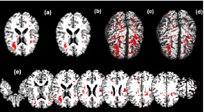
version of this article. . . 19 2.7 ADHD data analysis results. Top panels: significant regions in
the brain where there exists a morphological difference between children with ADHD and children who do not have the disorder, based on a 95% credible interval. Panel (a) is a selected axial slice of the STM estimate overlaid on the Jacob template; (b) is the same selected slice showing the estimates of the spatial model with the transformation parameters Λ fixed and equal to 1 for all voxels also overlaid on the template; (c) and (d) are, respectively, the results of a 3D rendering of the STM and of the no transformation model both overlaid on the Jacob template. Bottom panel: (e) shows selected axial slices of the STM estimates overlaid on the template. Highlighted areas show the significant regions in the brain where there exists a morphological difference between children with ADHD and children who do not have the disorder. This figure
appears in color in the electronic version of this article. . . 20 3.1 Figure copied from (Kolda and Bader, 2009b). Panel (a)
illus-trates the CP decomposition of a three way array as a sum of R
components of rank-one tensors, i.e. X ≈PRr=1ar◦br◦cr. . . 26 3.2 Trace plots in 9 randomly chosen voxels in the white matter RAVENS
map by using Bayesian tensor decomposition withR = 20. The trace plots indicate that the Markov chain converges after around
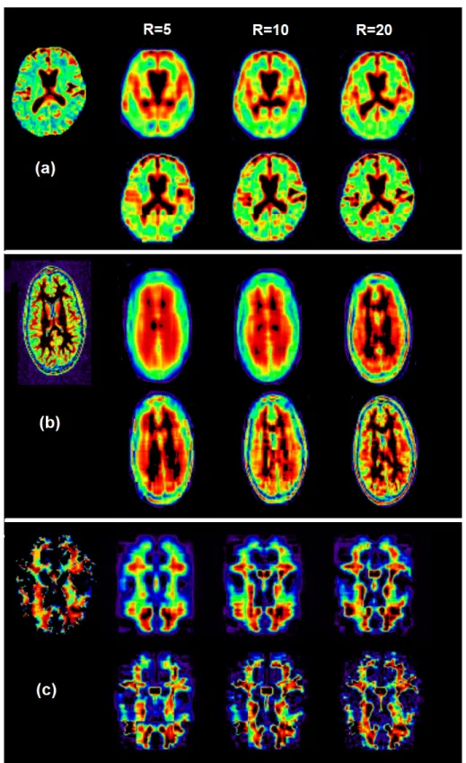
1000 iterations. . . 34 3.3 Simulation 1 for Bayesian tensor decomposition results: panel
(a): DTI image; panel (b): white matter RAVENS map; and panel (c): T1-weighted image In each row, the first image represents an axial slice of the original image and from left to right we have the
3.4 Results of the 2-D imaging example: (a):X0(0); (b):X0(1)−X0(0); (c): the simulated image from a randomly selected subject from group 1; (d): the estimated projectionP. Panels (e) and (g) are the posterior mean of the quantityP =
Λ;A
(1)
,A(2),B
for BTRM withS = 4and the no-partition model withS = 1, respectively. Panels (f) and (h) are, respectively, the95%credible interval ofP for BTRM(S= 4) and BTMR(S = 1) revealing the true underlying
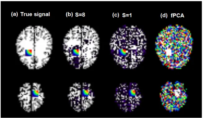
location, where differences between both groups exist. . . 37 3.5 Results of the 3-D image example. In each panel, we show axial
views of the 2 true signal regions and a 3D render of the results overlaid on the template G0 from left to right. Panel (a) show the true effect signalX0. Panels (b) and (c) present the posterior mean of the quantity P =
Λ;A
(1)
,A(2),A(3),B
for TPRMs with S = 8 and with S = 1, respectively. Panel (d) shows the results for fPCA. Both TPRMs are able to recoverX0, whereas
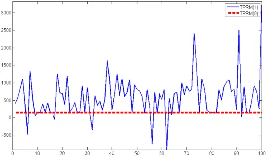
fPCA does not. . . 39 3.6 DIC results of 100 simulated examples. Straight line indicates
the non-partition model TPRM(S = 1) and dotted line indicates partition TPRM(S = 8). The later model is preferred in the majority
of generated datasets. . . 40 3.7 Axial slices of the posterior mean estimates for the projection
P =
λ;A
(1)
,A(2),A(3),B
for the TPRM (panel (b)) and the estimated projection for fPCA (panel (a)). The colors indicate how strong the differences are between children with ADHD and control. The 3 slices on the right indicate a possible right frontal lobe region, in both models. A strong difference seems to exist in the left frontal lobe and left parietal lobe when observing the TPRM model but not in the fPCA model. The chain was generated with 5000 iterations
and the burn-in period is of 3000. . . 42 3.8 ADHD data analysis results. Panels (a) and (b) are, respectively,
the results of a 3D rendering of the 90% and 95% credible intervals for the projectionP =
λ;A
(1)
,A(2),A(3),B
both overlaid on the Jacob template. Panel (c) and (d) are selected axial slices of the credible intervals (95%and90%, respectively). We detect two large regions of interest, where morphological differences exist,
4.2 Trace plots of the projectionP =S sP
(s)
, whereP(s) =
A(s)
T b(s), for9random voxels of the partition model withNs = 8, R = 50, after a burn-in period of 500. The plots indicate a fast convergence
of the chain. . . 54 4.3 Simulation results for the Bayesian sparse partition factor model
(BSPFM) with Ns = 18,Ns = 8 and Ns = 1. Panel (a) shows the true underlying signalX1 overlaid on the templateX0; panel (b) shows the estimated projection for the PCA model and panels (c)-(e) are posterior mean of the projection for the partition and
non-partition model, all results overlaid on the templateX0. . . 55 4.4 ADHD data analysis results for the Bayesian partition partial factor
model (BPPFM) withNs = 24partitions and rankR= 200. Panel (b) shows the results of the posterior mean of the projectionP and panel (a) shows the estimated projection for the 2-stage PCA model. The colors indicate the strength of the differences between children
with ADHD and control. . . 58 4.5 ADHD data analysis results for the Bayesian partition partial factor
model (BPPFM) withNs = 24partitions and rankR= 200. Panel (a) and (b) show the results of a 3D rendering of the 95% and 90% credible intervals for the projection overlaid on the Jacob template, respectively; panels (c) and (d) are selected axial slices of the 90%
and 95% credible interval for the projection, respectively. . . 59 A.1 Sensitivity analysis ofΛ. Panels (a)-(d) represent the true pattern
ofβused to generate the images; (e)-(h): the posterior means of βobtained with (a, b) = (−2.0,2.5); (i)-(l): the posterior means ofβobtained with(a, b) = (−3.0,3.0); and (m)-(p): the posterior
means ofβwith(a, b) = (−3.5,3.5). . . 64 A.2 Trace plots ofνkfork = 0, . . . ,3after a burn-in of 50 iterations and
a total of 1000 MCMC iterations under the three scenarios of(a, b). Rows 1-3 correspond to(a, b) = (−2.0,2.5),(a, b) = (−3.0,3.0),
and(a, b) = (−3.5,3.5), respectively. . . 65 A.3 Trace plots ofβ,τσ andλfor the scenario(a, b) = (−3.5,3.5)at 4
random selected voxels. The results show fast convergence of the
MCMC chain for all parameters. . . 66 A.4 Posterior estimates ofβfor different values ofφk: (a)-(d): φk =
0.01; (e)-(h)φk = 0.1; (i)-(l)φk = 1; and (m)-(p):φk= 100. . . 68 A.5 Posterior estimates ofβunder different specifications ofHk. Panels
A.6 The posterior estimates ofβfor the true model withλd= 1for all
d∈ D. . . 70
A.7 The posterior estimated image Λ =ˆ {λˆd : d ∈ D} for the true
underlying model withλd= 1for alld∈ D. . . 70 A.8 The posterior mean, the posterior standard deviation (SD), and
the standardized value (mean/SD) images corresponding to the
interceptβ0are shown from the left to the right, respectively. . . 71 A.9 The posterior mean, the posterior standard deviation (SD), and the
standardized value (mean/SD) images corresponding to the gender
β1are shown from the left to the right, respectively. . . 71 A.10 The posterior mean, the posterior standard deviation (SD), and the
standardized value (mean/SD) images corresponding to the ageβ2
are shown from the left to the right, respectively. . . 71 A.11 The posterior mean, the posterior standard deviation (SD), and the
standardized value (mean/SD) images for the ADHD statusβ3are
shown from the left to the right, respectively. . . 72 A.12 Illustration of the one-way dependency structure of the functions. . . 73 A.13 Simulation results obtained by runningMainSTM.m. Panels
(a)-(d) represent the pattern ofβused to generate the images; panels (e)-(h) are estimatedβobtained from the least squares estimator in
Matlab; panels (i)-(l) are the posterior mean ofβobtained from our STM. . . 76 A.14 Simulation results: the true Λ = {λd, d ∈ D}pattern in the left
panel and the estimated pattern in the right panel. Estimated image is smoother compared with the true image due to the nature of the
CHAPTER 1: INTRODUCTION
In the past few decades, medical imaging technologies have been improving and a number of expanding modalities are creating impressively accurate and detailed images for less invasive and more precise methods of diagnosis. Although these advances are allowing researchers and clinicians to gain insights of unprecedented quality on the cerebral anatomical structures, connectivity patterns and functional properties, it also brings the challenge of developing automatic methods to categorize and classify brain responses, identify abnormalities in the brain, understand mental thoughts, and reveal important effects of environmental and genetic factors on brain structure and function, among many others.
To face these challenges, classical statistical tools need to be adapted to more complex data structures of typical neuroimaging studies. These data usually take the form of mul-tidimensional arrays with intricate spatial correlation and functional changes that evolve over time. This dissertation makes further contributions to the development of statistical tools motivated by these challenges. More specifically, we develop methods to characterize varying associations between ultra-high dimensional imaging data and low-dimensional response variables.
The tools originated by this research fall into two categories of solutions to establish association between multidimensional images and clinical outcomes and are described as follows.
1.1 Voxel-wise models
flawed; (ii) the voxels are treated as independent units and the spatial structure of the brain is ignored until the very last stage, when a correction is made on the test statistics.
Chapter 2 simultaneously addresses these issues by developing a class of spatial trans-formation models (STM) to model the spatially varying associations between imaging measurements in a three-dimensional (3D) volume (or 2D surface) and a set of covariates. The proposed STM includes a spatially varying Box-Cox transformation model for dealing with the issue of non-Gaussian distributed imaging data and a Gaussian Markov random field model to incorporate spatial smoothness of the imaging data.
1.2 Low-rank regression models
A different perspective is to consider imaging data to predict a scalar response. However, a typical neuroimaging study, with magnetic resonance imaging (MRI), produces images of size256×256×256, with approximately16.5million voxels. Most models are compromised by this ultra-high dimensionality.
A possible solution is to integrate supervised (or unsupervised) dimension reduction techniques with various standard regression models. Given the ultra-high dimension of imaging data, however, it is imperative to use some dimension reduction methods to extract and select “low-dimensional” important features.
The dimension reduction step is often perform by applying principal component analysis (PCA) or high-order tensor decompositions, e.g. CP or Tukey. Further, the top compo-nents extracted on the decomposition are used to predict a clinical outcome. A crucial assumption is that the leading components obtained from these decompositions capture the most important features of the multi-dimensional array. However, neuroimaging data are extremely noisy, and regions affecting the outcome are small and often clustered together. As a consequence, it is likely that “effect” regions will not be noticed.
MRI image of size256×256×256, and assume we partition the image into163 = 4,096 subarrays of size16×16×16. If we reduce each16×16×16subarray into a small number of components, not only the the total number of reduced features drop to a manageable level, but also we are more likely to capture small clustered effect regions. Both solutions are formulated as supervised hierarchical models, and an efficient Markov chain Monte Carlo algorithm is developed.
1.3 Outline of Thesis
CHAPTER 2: BAYESIAN SPATIAL TRANSFORMATION MODELS 2.1 Introduction
The emergence of various imaging techniques has enabled scientists to acquire high-dimensional imaging data to closely explore the function and structure of the human body in various imaging studies. Several common imaging techniques include magnetic resonance image (MRI), functional MRI, diffusion tensor image (DTI), positron emission tomography (PET), and electroencephalography (EEG), among many others. These imaging studies, such as the Alzheimer’s Disease Neuroimaging Initiative (ADNI), are essential to understanding the neural development of neuropsychiatric and neurodegenerative disorders, the normal brain and the interactive effects of environmental and genetic factors on brain structure and function, among others. A common feature of all these imaging studies is that they have been generating many very high dimensional and complex data sets.
There is a great interest in developing voxel-wise methods to characterize varying asso-ciations between high-dimensional imaging data and low-dimensional covariates (Friston, 2007; Lindquist, 2008; Lazar, 2008; Li et al., 2011). These methods usually fit a general linear model to the imaging data from all subjects at each voxel as responses and clinical variables, such as age and gender, as predictors. Subsequently, a statistical parametric map of test statistics orp-values across all voxels (Lazar, 2008; Worsley et al., 2004) is generated. Several popular neuroimaging software platforms, such as statistical paramet-ric mapping (SPM) (www.fil.ion.ucl.ac.uk/spm/) and FMRIB Software Library (FSL) (www.fmrib.ox.ac.uk/fsl/), include these voxel-wise methods as their key statistical tools.
et al., 2005; Worsley et al., 2004; Zhu et al., 2009). This distributional assumption is important for the valid calculation ofp−values in conventional tests (e.g., F test) that assess the statistical significance of parameter estimates. Moreover, methods of random field theory (RFT) that account for multiple statistical comparisons depend strongly on the parametric assumptions, as well as several additional assumptions (e.g., smoothness of autocorrelation function).
Second, the Gaussian assumption is known to be flawed in many imaging datasets (Ashburner and Friston, 2000; Salmond et al., 2002; Luo and Nichols, 2003; Zhu et al., 2009). It is common to use a Gaussian kernel with the full-width-half-max (FWHM) in the range of 8-16mm to account for registration errors, to make the data normally distributed and to integrate imaging signals from a region, rather than from a single voxel. However, recent research has shown that varying filter sizes in the smoothing methods can result in different statistical conclusions about the activated and deactivated regions, and spatial smoothing biases the localization of brain activity. Thus, it can result in misleading scientific inferences (Jones et al., 2005; Sacchet and Knutson, 2012).
The aim of this paper is to develop a class of spatial transformation models (STMs) to simultaneously address the issues discussed above for the spatial analysis of neuroimaging data given a set of covariates. Our spatial transformation model is a hierarchical Bayesian model. First, we use a Box-Cox transformation model on the response variable assuming an unknown transformation parameter in order to satisfy the normality assumption in the imaging data, and then develop a regression model to characterize the association between the imaging data and the covariates. Second, we use a Gaussian Markov random field (GMRF) prior to capture the spatial correlation and spatial smoothness among the regression coefficients in the neighboring voxels. We develop an efficient Markov chain Monte Carlo (MCMC) algorithm to draw random samples from the desired posterior distribution. Our simulations and real data analysis demonstrate that STM significantly outperforms the standard voxel-wise model in recovering meaningful regions.
The rest of this paper is organized as follows. In Section 2.2, we introduce the STM and its associated prior distributions and Bayesian estimation procedure. In Section 2.3, we compare STM with the standard voxel-wise method using simulated data. In Section 2.4, we apply STM to a real imaging dataset on attention deficit hyperactivity disorder (ADHD). Finally, in Section 5, we present some concluding remarks.
2.2 Model
2.2.1 Model Description
We propose a class of spatial transformation models consisting of two major components: a transformation model and a Gaussian Markov random field model. The transformation model is developed to characterize the association between the imaging measures and the covariates at anyd∈ Dand to achieve normality. Since most imaging measures are positive, we consider the well-known Box-Cox shifted power transformation (Box and Cox, 1964) throughout. Extensions to other parametric transformations are trivial (Sakia, 1992). Let
yi(d)(λ)be the Box-Cox transformation ofyi(d)given by
yi(d)(λ)=
{(yi(d) +c0)λ−1}/λ, if λ 6= 0,
log(yi(d) +c0), if λ = 0,
wherec0 is prefixed and chosen such thatinfi,d(yi(d))>−c0. Our Box-Cox transformation model is given by
y(λd)
i (d) = x
T
i β(d) +εi(d) for d∈ D, (2.1)
whereβ(d) = (β1(d), . . . , βp(d))T is ap×1vector of regression coefficients of interest,xi is ap×1vector of observed covariates for subjecti, andε(d) = (ε1(d), . . . , εn(d))T is an
n×1vector of measurement errors and follows aNn(0, σ2(d)In)distribution, in whichIn is ann×nidentity matrix.
The Gaussian Markov random field (GMRF) model is proposed to capture the spatial smoothness and correlation for each component of{β(d) :d ∈ D}across all voxels. For
with the imaging data. Specifically, we assume that
βk ∼N(0, νk−1(IND+φkHk)
−1),
whereνk > 0and φk > 0are, respectively, scale and spatial parameters. When φk = 0, the elements of βk are independent, whereas when the value of φk is large, the model approaches an intrinsic autoregressive model (Ferreira and De Oliveira, 2007; Rue and Held, 2005). The known matrixHk ={hk(d, d0)}is anND×ND matrix allowing the modeling of different patterns of spatial correlation and smoothness. LetN(d)be a set of neighboring voxels of voxeldin a given neighborhood system. Using the properties of GMRF (Rue and Held, 2005), the full conditional distribution ofβk(d)can be written as
βk(d)|β(k),[d], νk, φk ∼N
φkPd0∈N(d)hk(d, d0)βk(d0)
1 +φkhk(d, d)
, 1
νk[1 +φkhk(d, d)] !
, (2.2)
whereβk,[d]contains allβk(d0)for alld0 ∈ Dexceptd. The conditional mean ofβ(k)(d)is a weighted average of theβk(d0)values in the neighboring voxels ofd. As the number of neighboring voxels increases, the conditional variance decreases (Ferreira and De Oliveira, 2007).
A challenging issue is how to specify Hk = {hk(d, d0)} for each βk in order to explicitly incorporate the spatial correlation and smoothness among neighboring voxels. We set
hk(d, d0) =
P
d0∈N(d)ωk(d, d0)2, for d=d0, −ωk(d, d0)21(d0 ∈N(d)), for d6=d0,
whereωk(d, d0)are some pre-calculated weights and1(A)is the indicator function of a set A. For everyφk ≥0,(IND +φkHk)
−1 is diagonally dominant and thus positive definite. For computational efficiency, we choose a relatively small neighborhood for each voxeld
d, d0 ∈ D. Ideally, ω(d, d0) should contain some similarity information, such as spatial distance and imaging similarity, between voxelsdandd0. The simplest example ofωk(d, d0) is ωk(d, d0) = K(||d−d0||2), whereK(u) = exp (−0.5u2)1(u ≤ r0). Other choices of
ωk(d, d0)are definitely possible. For instance, one may borrow information learned from other imaging modalities in order to construct the similarity betweendandd0.
2.2.2 Priors
We first consider the priors for the remaining parameters in the first level of model (2.1). Letτd = (σ2(d))−1 and U(−a, b)denote the uniform distribution on the interval(−a, b). We specifically assume that ford∈ D,
τd∼Gamma(δ0/2, γ0/2) and λd∼U(−a, b).
For the second level parameterν= (ν1, . . . , νp), we assume fork= 1, . . . , p
νk ∼Gamma(nν/2, nνs2ν/2),
where nν and s2ν are hyperparameters. The choice of Gamma priors for the precision parameters is common in the literature since it maintains conjugacy (Chen et al., 2000). Other choices areπ(τd) =τd−11(τd≥ 0)andπ(νk) =νk−11(νk ≥0), which are improper but in both cases lead to a proper posterior distribution. The uniform prior for the transformationλd was first introduced by Box and Cox (1964) and later adopted by several authors (Sweeting, 1984; Gottardo and Raftery, 2006).
2.2.3 Posterior Computation
the higher level parameters first can result in an improvement of the speed of convergence. Details pertaining to each step are presented below.
(i) Update each component ofν = (ν1, . . . , νp)from its full conditional distribution,
p(νk|−)∼Gamma(0.5n∗νk,0.5n
∗
νks
∗2 νk),
whereνk∗ =ND +nν andn∗νs∗ν2 =nνs2ν+ PND
j=1βk(j)2+φkβTkHkβk.
(ii) Updateβk(d), k= 1, . . . , p, for each voxeld∈ Dfrom its full conditional distribution,
p(βk(d)|−)∼N µβk(d), σ
2 βk(d)
,
whereσ2β
k(d) = (τd
P ix
2
ik+θk(d))−1 and
µβk(d) = σ
2
βk(d){τd
X
i
[y(λd)
i (d)− X
l6=k
xilβ (m)
l (d)]xik+θk(d)mk(d)}.
Moreover,β(m)(d) ={βl(m)(d);l= 1, . . . , p}is the estimated value ofβ(d)obtained in the previous iteration of the Gibbs sampler andθk(d)andmk(d)are, respectively, the inverse of the variance and the mean of the Gaussian distribution in (2.2).
(iii) Updateτσ(d)for each voxeld∈ Dfrom its full conditional distribution
p(τσ(d)|−)∼Gamma
1
2(n+δ0), 1 2
X
i
(y(λd)
i (d)−x T iβ(d))
2+γ 0
!
.
(iv) Updateλdfor each voxeld∈ Dfrom its full conditional distribution
p(λd|−)∼ Y
d∈D
exp
( −τd
2
X
i
(y(λd)
i (d)−x T iβ(d))2
) ×
n Y
i=1
yλd−1
i (d)×(b+a)
The full conditional distribution of λd does not have a closed form, but sampling methods such as the Slice Sampler (Neal, 2003) or the Adaptive Rejection Metropolis Sampling (ARMS) (Gilks et al., 1995) can be used for such a purpose. The Metropolis-Hastings (MH) algorithm (Metropolis-Hastings, 1970) is also a very useful and easy algorithm for samplingλd. The MH algorithm proceeds as follows:
(a) Generateλpropd fromN(λd(t−1), δλ), whereδλ >0is a tuning parameter. (b) GenerateV fromU(0,1).
(c) Letα = min
1, p(λ
prop d |−)
p(λ(dt−1)|−)
. IfV ≤ α, then setλ(dt) =λpropd . Otherwise, set
λ(dt) =λ(dt−1).
Full conditional derivations details are presented in A. 2.3 Simulation Study
We carried out a simulation study to examine the finite-sample performance of the STM in establishing an association between the imaging data and a set of covariates. The goals of this simulation study are
(G.1) To examine the ability of STM in capturing different geometric patterns;
(G.2) To examine the posterior estimates of spatially varying transformation parameters under two scenarios, including a no transformation model;
(G.3) To investigate the sensitivity of STM to the specification ofφkand(−a, b);
(G.4) To investigate the sensitivity of STM to the matrixHk;
(G.5) To illustrate the fast convergence of the Gibbs sampler algorithm.
variable, and two columns indicating categories of a discrete variable. They were generated as follows: (i)xi1 is generated fromN(5,1); (ii) xi2 and xi3, respectively, represent the second and third category of a discrete uniform random variable generated from three possible values, each of them representing a category and defined byxiq =1(Category q)− 1(Category 1)for q = 2,3(Pasta, 2005). We generated the values of the transformation parametersλdfrom a discrete uniform random variable taking0.5,1, or2. The generatedΛ structure is presented in the left panel of Figure 2.1. The parameters inβare chosen to have a strong spatial correlation and their images are presented in the panels (a)-(d) of Figure 2.2.
For the hyperparameters ofβ, we chose a noninformative prior for eachνkby setting
nν = 10−3 ands2ν = 1. As for the entries of the matrixHk, we set it as in (2.3) and took the weights as ωk(d, d0) = K(||d−d0||2), whereK(u) = exp −12u2
1(u ≤ r0)andr0 = 2. For each parameterτσ, we chose noninformative priors by settingδ0 = 10−3 andγ0 = 10−3. We fixedφkat10, which indicates a strong spatial dependency among the components of eachβ(k), and then we seta=b= 3for the hyperparameters ofλd.
For each simulated dataset, we ran the Gibbs sampler for 1,000 iterations with 50 burn-in iterations. For the simulated examples, each iteration of the Markov chain takes approximately 2.5 seconds when running on a laptop with an i7 processor, 2.67GHz, and 8.0 GB of RAM. We summarize some simulation results based on some selected simulation scenarios below, while some additional results obtained from different simulation scenarios are considered in the Appendix A.
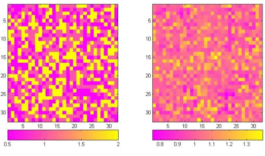
First, Figure 2.1 reveals that the estimated and true structures ofΛ={λd, d∈ D}show great similarity with each other. As expected, the estimated image Λˆ = {λˆd, d ∈ D}is smoother than the trueΛ={λd, d∈ D}since aU(−3,3)prior is assumed forλd, allowing
λdto be sampled within this interval.
Figure 2.1: Simulation results: the trueΛ={λd, d∈ D}pattern in the left panel and the estimated pattern in the right panel. Estimated image is smoother compared with the true image due to the nature of the uniform distribution assumeda priori. This figure appears in color in the electronic version of this article.
across all voxels (panels (i)-(l)). Figure 2.2 reveals that the voxel-wise linear model and STM (2.1) withλdfixed at1cannot capture the pattern of true coefficient images. In contrast, STM (2.1) substantially improves the estimation of the coefficients, recovering their true geometric patterns, as observed in Figure 2.2, panels (m)-(p). Moreover, the STM is robust to the choices of the hyperparametersφkand(−a, b). Furthermore, the correct specification of the matrixHkcan yield good estimates if a reasonable neighborhood system is chosen. Finally, even if the true underlying model does not require spatial transformation parameters, STM can still provide good estimates ofβ.
Figure 2.3: Trace plots forβ,τσ andλfor a randomly generated voxel. The results are for a 1000 iterations of the MCMC algorithm and a burn-in sample of 50. The trace plots indicate a fast convergence of the algorithm, confirming its efficiency and good mixing properties. This figure appears in color in the electronic version of this article.
2.4 Application to the ADHD dataset
Our model is applied to the Attention Deficit Hyperactivity Disorder data, obtained from the ADHD-200 Consortium,(http://fcon 1000.projects.nitrc.org/indi/adhd200), a self-organized initiative where members from institutions around the world provide de-identified, HIPAA compliant imaging data. The goal of the project is to accelerate the scientific community’s understanding of the neural basis of ADHD, which is one of the most common childhood disorders affecting at least 5-10% of school age children and is associated with substantial lifelong impairment. The symptoms include difficulty staying focused and paying attention, difficulty controlling behavior, and hyperactivity (over-activity).
(Magnetization-prepared Rapid Acquisition with Gradient Echo) technique. The original T1-weighted images have size256×256×198mm3and voxel size of1.0×1.0×1.0mm3.
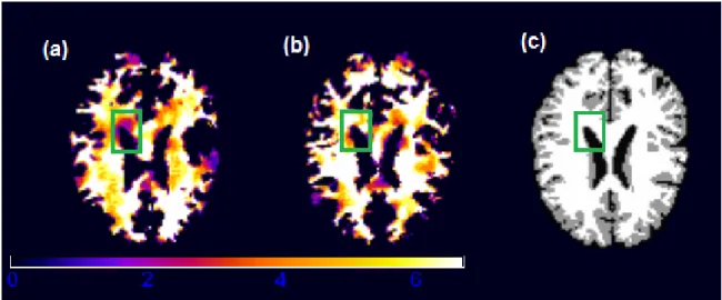
For each subject, the images were first downsampled to the size of128×128×99mm3. This process reduces the number of voxels while maintaining the image features and proper-ties. Next, the images were processed using HAMMER (Hierarchical Attribute Matching Mechanism for Elastic Registration), a free pipeline developed by the Biomedical Research Imaging Center at UNC (available for downloading athttp://www.hammersuite.com). The processing steps include skull and cerebellum removal, followed by tissue segmentation to identify the regions of white matter (WM), gray matter (GM) and cerebrospinal fluid (CSF). Then, registration was performed to warp the subject to the space of the Jacob template (Kabani et al., 1998; Davatzikos et al., 2001). Finally, a RAVENS map was calculated for each subject. The RAVENS methodology precisely quantifies the volume of tissue in each region of the brain. The process is based on a volume-preserving spatial transformation that ensures that no volumetric information is lost during the process of spatial normalization. In Figure 2.4, we illustrate the white matter RAVENS images for two randomly selected subjects (panels (a) and (b)). These images were registered to the space of the template shown in panel (c). When we compare subjects in panels (a) and (b) of Figure 2.4, the image from the subject in panel (b) shows higher brightness inside the green square, reflecting the fact that relatively more white matter is presented in that particular region relative to the template.
We fitted model (2.1) with the white matter RAVENS images as responses and the covariate vector containing intercept, gender, age (previously standardized) and ADHD diagnostic status (1 for ADHD and -1 for control). Our interest is to identify morphological differences in the brain that are associated with the ADHD outcome, while adjusting for age and gender. As in the simulation study, for the hyperparameters of β, we chose a noninformative prior for each νk by settingnν = 10−3 and s2ν = 1. We fixedφk = 10 and setωk(d, d0) =K(||d−d0||2), whereK(u) = exp −12u2
Figure 2.4: White matter RAVENS map for two randomly selected children from the ADHD study. The image from subject b shows a higher brightness inside the square, reflecting the fact that for the brain of subject b, relatively more white matter was forced to fit the same template (panel (c)) at that particular region. This figure appears in color in the electronic version of this article.
each parameterτd, we chose a noninformative prior by settingδ0 = 10−3 andγ0 = 10−3. For the transformation parameters λd, we set a = b = 2. We ran the Gibbs sampler for 1,000 iterations with 50 burn-in iterations. We calculated the posterior mean and a
95%credible interval for the coefficient associated with ADHD outcome at each voxel. A detailed discussion of credible intervals and its relation to the frequentist confidence interval is provided in Bayarri and Berger (2004). To detect important regions of interest, we created a5%threshold map by mapping whether the 95%credible interval at each voxel contains0
or not. Finally, we also fitted a no-transformation model, which is the STM withλdfixed at
1for all voxels.
transformation parameters are different from1for nearly70%of the voxels, based on a 95% credible interval (Figure 2.6, panel (d)).
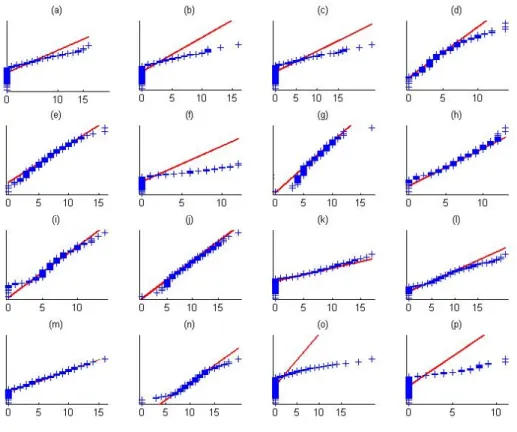
Figure 2.5: ADHD data analysis results: normal probability plots of sixteen random voxels revealing that the imaging measurements extracted from the RAVENS map deviate from the Gaussian distribution. This figure appears in color in the electronic version of this article.
We then mappedΛˆ into the template to observe how the transformation parameter varies across the brain. If morphological differences exist in the regions where the transformation parameters are significantly different from 1, then analyzing the imaging data using the standard voxel-wise linear model may lead to spurious conclusions. On the other hand, if the transformation parameters are close to 1in some regions, the estimates of the STM will be similar to those of the standard voxel-wise linear model in the regions. However, in practice, the location of such regions is unknown.
phological differences exist, including the right frontal lobe, the left frontal lobe and left parietal lobe. The frontal lobe has been implicated in planning complex cognitive behavior, personality expression, decision making and moderating social behavior (Yang and Raine, 2009) and morphological differences in this region were previously identified in children with ADHD (Sowell et al., 2003). Although the right frontal lobe is noticeable in all panels of Figure 2.7, the left frontal lobe cannot be seen for the no-transformation model in panel (d) of Figure 2.7. Thus, without the use of data transformations, we may miss some biologically meaningful regions of interest.
Figure 2.7: ADHD data analysis results.Top panels: significant regions in the brain where there exists a morphological difference between children with ADHD and children who do not have the disorder, based on a 95% credible interval. Panel (a) is a selected axial slice of the STM estimate overlaid on the Jacob template; (b) is the same selected slice showing the estimates of the spatial model with the transformation parametersΛfixed and equal to
2.5 Discussion
CHAPTER 3: TENSOR PARTITION REGRESSION MODELS 3.1 Introduction
The aim of this paper is to develop a novel tensor partition regression modeling frame-work (TPRM) in order to use high-dimension imaging data, denoted byx, to predict a scalar response, denoted byy. The scalar responseymay include cognitive outcome, disease status, and the early onset of disease, among others. In various neuroimaging studies, imaging data are often measured at a large number of grid points in a three (or higher) dimensional space and have a multi-dimensional tensor structure. Without loss of generality, we use x= (xj1···jD)∈R
J1×···×JD to denote an orderDtensor, whereD≥2. Vectorizingxleads
to a (QDk=1Jk)×1vector. Examples of x include magnetic resonance imaging (MRI), diffusion tensor imaging (DTI), and positron emission tomography (PET), among many others. These advanced medical imaging technologies are essential to understanding the neural development of neuropsychiatric and neurodegenerative disorders.
family of tensor regression models has been developed to preserve the spatial structure of imaging tensor data, while achieving substantial dimensional reduction (Zhou et al., 2013).
The second set of solutions adopts functional linear regression (FLR) approaches, which treat imaging data as functional predictors. However, since most existing FLR models focus on one dimensional curves (M¨uller and Yao, 2008; Ramsay and Silverman, 2005), generalizations to two and higher dimensional images, however, is far from trivial and requires substantial research (Reiss and Ogden, 2010a). For instance, most estimation methods of FLR based on the fixed basis functions (e.g., tensor product wavelet) are required to solve an ultra-high dimensional optimization problem and suffer the same limitations as those of HSR.
The third set of solutions usually integrates supervised (or unsupervised) dimension reduction techniques with various standard regression models. Given the ultra-high dimen-sion of imaging data, however, it is imperative to use some dimendimen-sion reduction methods to extract and select ’low-dimensional’ important features, while eliminating most redun-dant features (Johnstone and Lu, 2009; Bair et al., 2006; Fan and Fan, 2008; Tibshirani et al., 2002; Krishnan et al., 2011). Most of these methods first carry out an unsupervised dimension reduction step, often by principal component analysis (PCA), and then fit a regression model based on the top principal components (Caffo et al., 2010). Recently, for ultra-high tensor data, higher order tensors decompositions (e.g. parallel factor analysis and Tucker) have been extensively proposed to extract important information of neuroimaging data (Martinez et al., 2004; Beckmann and Smith, 2005). Although it is intuitive and easy to implement such methods, it is well known that the features extracted from PCA and Tucker can be irrelevant to the response. Similar comments also hold for FLR based on the functional PCA basis functions.
sub-tensor covariates; (ii) a canonical polyadic decomposition model of reducing sub-sub-tensor covariates to low-dimensional feature vectors; and (iii) a generalized linear model of using the feature vectors to predict clinical outcomes. Moreover, a sparse inducing normal mixture prior is used to select informative feature vectors. Among the four components of TPRM, the key novelty of TPRM lies in the components (i) and (ii).
The first two components (i) and (ii) are designed to specifically address the three key features of neuroimaging data: low signal to noise ratio, the spatially clustered effect, and the tensor structure of imaging data. The neuroimaging data are often very noisy, while the ‘activated’ (or ‘effect’) brain regions associated with the response are usually clustered together and their size can be very small. In contrast, a crucial assumption for the success of most matrix/array decomposition methods (e.g., singular value decomposition) is that the leading components obtained from these decomposition methods capture the most important feature of a multi-dimensional array. Under TPRM, the ultra-high dimensionality of imaging data is dramatically reduced by using the partition model. For instance, let’s consider a standard256×256×2563D array with 16,777,216 voxels, and its partition model with
323 = 32,768 sub-arrays with size8×8×8. If we reduce each8×8×8into a small number of components by using component (ii), then the total number of reduced features is aroundO(104). We can further increase the size of each subarray in order to reduce the size of neuroimaging data to a manageable level, resulting in efficient estimation.
3.2 Methodology 3.2.1 Preliminaries
We review several basic facts of tensor (Kolda and Bader, 2009b). A tensor x = (xj1...jD)is a multidimensional array, whose orderDis determined by its dimension. For
instance, a vector is a tensor of order 1 and a matrix is a tensor of order 2. The inner productbetween two tensorsX = (xj1...jD)andY = (yj1...jD)in<
J1×...×JD is the sum of
the product of their entries given by
hX,Yi =
J1 X
j1=1
. . .
JD
X
jD=1
xj1...jDyj1...jD.
The outer productbetween two vectorsa(1) = (a(1)j1 )∈ <J1 anda(2) = (a(2) j1 )∈ <
J2 is a matrixM = (mj1j2)of sizeJ1×J2with entriesmj1j2 =a
(1) j1 a
(2)
j2 . A tensorX ∈ <
J1×...×JD
is arank one tensorif it can be written as an outer product of Dvectors such thatX =
a(1) ◦a(2). . .◦a(D), wherea(k) ∈ <Jk fork = 1,· · · , D. Moreover, the parallel factor
analysis, also known as PARAFAC orCP decomposition, factorizes a tensor into a sum of rank-one tensors such that
X ≈ R X
r=1
λra(1)r ◦a (2)
r ◦. . .◦a (D)
r , (3.1)
where a(rk) = (a(jkkr)) ∈ <Jk for k = 1, . . . , D and r = 1, . . . , R. See Figure 3.1 for an illustration of a 3D array.
We need the following notation throughout the paper. Suppose that we observe data {(yi,Xi,zi) : i = 1, . . . , N}fromn subjects, where Xi are tensor imaging data, zi is a
Figure 3.1: Figure copied from (Kolda and Bader, 2009b). Panel (a) illustrates the CP decomposition of a three way array as a sum of R components of rank-one tensors, i.e. X ≈PRr=1ar◦br◦cr.
follows:
˜
X =kΛ;A(1), . . . ,A(D),Gk or xj1,...,jD,i =
R X
r=1
λra (1) j1ra
(2) j2r. . . a
(D)
jDrgir. (3.2)
whereΛ =diag(λ1,· · ·, λR),A(d)= [a(1d)a (d) 2 . . .a
(d)
R ]ford= 1, . . . , D, andG= (gir)is called the factor matrix.
3.2.2 Tensor Partition Regression Models
Our interest is to develop TPRM for establishing the association between responsesy
and their corresponding imaging covariatesX and clinical covariatesZ. The first component of TPRM is a partition model of dividing the high-dimensional tensor X˜ into S disjoint sub-tensor covariatesX˜(s), that is
˜
X =∪S s=1X˜
(s)
and X˜(s)∪X˜(s0) =∅.
(3.3)
Although the size ofX˜(s) can vary acrosss, it is assumed that without loss of generality,
˜
X(s) ∈ Rp1×...×pD and the size ofX˜(s) is homogeneous such thatS =QD
assumed that for eachs, we have
˜
X(s) =kΛ
s;A(1)s ,A (2)
s , . . . ,A (D)
s ,Gsk+E(s), (3.4)
whereΛs =diag(λ(1s),· · · , λ(Rs))consists of the weights for each rank of the decomposition in (3.4), A(sd) ∈ <pd×R are the factor matrices along thed-th dimension ofX, andG
s ∈ <N×Ris the factor matrix along the subject dimension. It is assumed that the elements of E(s) = (e(s)
j1...jDi)are measurement errors ande
(s)
j1...jDi ∼N(0,(τ
(s))−1). The elements ofG s
capture the major variation inX(s)due to subject differences, while the common structure among the subjects is absorbed into the factor matricesA(sd)ford= 1, . . . , D(Kolda and Bader, 2009a).
There are two key advantages of using (3.3) and (3.4). First, the use of the partition model (3.3) allows us to concentrate on the most important local features of each sub-tensor, instead of the major variation of the whole image, which may be unassociated with the response of interest. In many applications, although the effect regions associated with responses may be relatively small compared with the whole image, their size can be comparable with that of each sub-tensor. Therefore, one can extract more informative features associated with the response with a high probability. Second, the use of the canonical polyadic decomposition model (3.4) can substantially reduce the dimension of original imaging data. Recall the discussions in Section 1 that the use of8×8×8sub-tensors can substantially reduce imaging size at a scale ofO(103).
The third component of TPRM is a generalized linear model that links scalar responsesyi and their corresponding reduced imaging featuresGsand clinical covariateszi. Specifically,
yigivengi andzifollows an exponential family distribution with density given by
whereh(·),η(·),T(·), and a(·)are pre-specified functions. Moreover, it is assumed that
µi =E(yi|gi,zi)satisfies
h(µi) = zTi γ+ S X
s=1
g(is)Tb(s), (3.6)
whereg(is) = vec(Gs)is the vectorization ofGs for all s, andγ andb(s) are coefficient vectors associated withziandg
(s)
i , respectively. 3.2.3 Prior Distributions
We consider the priors on the elements ofb(rs). The magnitude of SR can be much larger thanN even for smallR, and thus model (3.6) is non-identifiable. To deal with this identifiability issue, bimodal sparsity promoting priors are key elements and have been the subject of extensive research (Mayrink and Lucas, 2013; George and McCulloch, 1993, 1997). We assume the following hierarchy:
br(s)|δr(s), σ2 ∼ (1−δr(s))F(b(rs)) +δr(s)N(0, σ2), (3.7)
δ(rs)|π ∼ Bernoulli(π) and π ∼Beta(α0π, α1π),
where F(·) is a pre-specified probability distribution. A common choice of F(·) is a degenerate distribution at0, leading to what is called the ‘spike and slab’ prior (Mitchell and Beauchamp, 1988). A different approach is to considerF =N(0, )with a very small
instead of putting a probability mass onb(rs) = 0. Thus,b(rs)’s are assumed to come from a mixture of two normal distributions. In this case, the hyperparameterσ2 should be large enough to give support to values of the coefficients that are substantively different from0, but not so large that unrealistic values ofb(rs)are supported. In this article, we opt for the latter approach.
this choice for the hyperparameters implies that its posterior mean is restricted to the interval
[1/3,2/3], a undesirable feature in variable selection. To fix this, we choose a “bathtub” shaped beta distribution, since a prior concentrating most of its mass in the extremes of the interval(0,1)is evidently more suitable for variable selection (Gonalves et al., 2013).
We consider the priors on the elements ofA((ds))r,gr(s),τ(s), andλ(rs). Ford= 1, . . . , D andr = 1, . . . , R, we assume
A((ds))r ∼N(0, p−d1Ipd), g
(s)
r ∼N(0,IN), τ(s) ∼Gamma(ν0τ, ν1τ), and λ(rs) ∼N(0, κ
−1),
whereIk be ak ×k identity matrix. Whenpdis large, the columns of the factor matrix
A((ds))rare approximately orthogonal, which is consistent with their role in the decomposition (3.1). However, we only impose that the columns of the factor matrices span the space of the principal vectors, without explicitly requiring orthonormality (Xinghao Ding and Carin, 2011).
For the remaining elements of TPRM, we assume
γ∼N(0, υ−1Iq) and υ ∼Gamma(ν0υ, ν1υ).
3.2.4 Posterior Inference
LetA(d)= [A((1)d), . . . ,A((dS))],G= [G1, . . . ,GS],B = [b(1), . . . ,b(S)],Λ= [Λ1, . . . ,ΛS], andτ = [τ(1), . . . , τ(S)]. Considerθ = {A(1). . . ,A(D),G,Λ,τ,γ, υ,B,δ, π}. A Gibbs sampler algorithm is used to generate a sequence of random observations from the joint posterior distribution given by
p(θ|,X,y)∝p(y|θ,X)p(A(1). . . ,A(D),G,Λ,τ|X)p(B|y,G,δ)p(δ|π)p(π)p(γ|υ)p(υ).
As an illustration, we divide the whole image intoSequal sized regions and assume
yi ∼ Bernoulli(µi) with the link function h(·)being the probit function. By following Albert and Chib (1993), we define a normally distributed latent variable,wi, such that
wi ∼N(µi,1); yi =1(wi >0),
where1(·)is an indicator function of an event.
The complete Gibbs sampler algorithm proceeds as follows. (a.0) Generatew= (w1,· · · , wn)T from
wi|yi = 0 ∼1(wi ≤0)N(zTi γ+ S X
s=1
g(is)Tb(s),1),
wi|yi = 1 ∼1(wi ≥0)N(zTi γ+ S X
s=1
g(is)Tb(s),1).
(a.1) Updateτ(s)from its full conditional distribution
τ(s)| · · · ∼Gamma(ν0τ + (N D Y
d=1
pd)/2, ν1τ+ (1/2) X
i,j1,...,jD
(x∗ij1,...,jD(s))2),
wherex∗ij1,...,j3(s) = {X(s)− kΛ(s);A(1) s ,A
(2)
s , . . . ,A (D) s ,L
(s)k} ij1,...,j3
(a.2) Update{A(d)
s }jdrfrom its full conditional distribution given by
{A(d)
s }jdr| · · · ∼N
τ(s)hXb s(jd)
(−r),I s (−d)i
τ(s)hIs (−d),I
s
(−d)i+pd
, τ(s)hIs (−d),I
s
(−d)i+pd −1
!
,
whereIs
(−d)=kΛ
(s);A(1)
s , . . . ,A (d−1) s ,A
(d+1)
s , . . . ,A (D) s ,L
(s)k, b Xs
(−r)is given by
X(s)−kΛ(s);A(1) s ,A
(2)
s , . . . ,A (D) s ,L
(s) i k+kΛ
(s);{A(1)
s }:,r,{A(2)s }:,r, . . . ,{A(sD)}:,r,{L (s) i }:,rk,
andXb s(jd)
(a.3) Update{Ls}ir from its full conditional distribution given by
{Ls}ir| · · · ∼N
τ(s)hXb s(i) (−r),I
si
τ(s)hIs,Isi+N,(τ(s)hI
s,Isi+N)−1 !
,
whereIs =kΛ(s);A(1)
s , . . . ,A (D)
s k,Xb(s−r)is the same as above andXb s(i)
(−r)is a subten-sor fixed at thei-th entry along the subject dimension ofXb(s−r).
(a.4) UpdateΛ(s)from its full conditional distribution
λ(rs)| · · · ∼N τ(s)hXb s (−r),L
si
τ(s)hLs,Lsi+κ,(τ(s)hL
s,Lsi+κ)−1 !
,
whereLs =k1
R;A(1)s , . . . ,A (D) s ,L
(s)k
and1Ris a vector of ones of sizeR. (a.5) Updateδr(s) from its full conditional distribution
δ(rs) ∼bernoulli(˜p1/˜p1+ ˜p0),
wherep˜1 =πexp{−(1/2σ2)(b (s)
r )2}andp˜0 =πexp{−(1/2)(b (s) r )2}.
(a.6) Updateb(rs) from its full conditional distribution
b(rs)|δ(rs) = 1∼N(X
i
˜
wi(s)g(irs)/X
i
(g(irs))2+ 1/σ2,(X
i
(g(irs))2+ 1/σ2)−1),
b(rs)|δ(rs) = 0∼N(X
i
˜
wi(s)g(irs)/X
i
(g(irs))2+ 1/,(X
i
(gir(s))2+ 1/)−1),
wherew˜i(s) =wi−zTi γ− PS
s0=1g (s0)T
i b
(s0)+g(s)T ir b
(s) r . (a.7) Updateπfrom its full conditional distribution
π| · · · ∼beta(α0π+ X
s,r
δr(s), α1π+SR− X
s,r
(a.8) Updateγfrom its full conditional distribution
γ| · · · ∼N Σ∗−1ZTw∗,Σ∗−1,
whereΣ∗ =υIq+ZTZ and=w∗ =w−PSs=1g(is)Tb (s)
.
(a.9) Updateυ from its full conditional distribution
υ| · · · ∼Gamma ν0υ+q/2, ν1υ+ (γTγ)/2
.
All the tensor operations described in steps(a.1)−(a.4)can be easily computed using Bader et al. (2012), available for download at http://www.sandia.gov/ tgkolda/TensorToolbox/index-2.5.html.
3.3 Simulation Study
We carried out three sets of simulations to examine the finite-sample performance of TPRM and its associated Gibbs sampler algorithm.
3.3.1 Bayesian tensor decomposition
hyperparameters were chosen to reflect non-informative priors,ν0τ = 1,ν1τ = 10−2, and
κ= 10−6.
We run steps(a.1)−(a.4)of the Gibbs sampler algorithm in Section 3.2.4 for5,000
iterations. The efficiency of the proposed algorithm is observed through trace plots for 9 random voxels. Figure 3.2 shows the trace plots for the reconstructed white matter RAVENS map decomposed withR = 20. The proposed algorithm is efficient and presents a fast convergence.
At each iteration, we computed the quantityI =PSs=1
Λs;A
(1) s ,A
(2) s ,A
(3) s
for each rank and each partition. Subsequently, we computed the reconstructed image, defined asXˆ, and the posterior mean estimate ofIafter a burn-in sample of3,000. For each reconstructed imageXˆ, we computed its root mean squared error, RMSE =||X − X ||ˆ 2/
√
J1J2J3. We compare the RMSE for the Bayesian non-partition model, the partition, and the standard alternating least squares method (ALS) (Kolda and Bader, 2009a). Results are shown in Table 3.1. For the images considered in this study, the partition model gives the smallest RMSE, and the Bayesian decomposition gives a smaller RMSE when compared to the standard ALS. As expected, higher is the rank, smaller is the reconstruction error.
We illustrate the impostance of the partitions in Figure 3.3. Results are from an axial slice of the original images and the reconstructed images for ranksR = 5,10,and20for both non-partition (top panels) and partition models (bottom panels) for all three images considered in this section. We clearly see an improvement in reconstruction when the partitions are considered in the model.
3.3.2 A 2-dimensional image example
Figure 3.2: Trace plots in 9 randomly chosen voxels in the white matter RAVENS map by using Bayesian tensor decomposition withR= 20. The trace plots indicate that the Markov chain converges after around 1000 iterations.
T1-weighted WM RAVENS DTI
R=5 BayesianCP 45.3191 1.5853 3.1656e-004
ALS 45.3636 1.6013 3.2506e-004
Partition 37.3712 1.2178 2.0929e-004
R=10 BayesianCP 41.7018 1.4382 2.7367e-004
ALS 42.4350 1.4533 2.8247e-004
Partition 31.3836 1.0186 1.5748e-004
R=20 BayesianCP 37.1796 1.2885 2.2911e-004
ALS 38.3166 1.3166 2.3676e-004
Partition 25.1574 0.8085 1.1349e-004
Table 3.1: Root mean squared error for 3 different image modalities. The Bayesian decom-position outperforms the alternating least squares in each scenario. There is a smaller error measurement with an increase of the rankR.
a data set{(yi,Xi) :i= 1, . . . , n}withn = 200according to
whereXi,Ei = (ij1j2), andX0(yi)are32×32matrices andX0(0)andX0(1)−X0(0)are, respectively, shown in panels (a) and (b) of Figure 3.4. We independently generatedij1j2 from aN(0,402)generator forj
1, j2 = 1, . . . ,32. Panel (c) in Figure 3.4 shows a generated 2D image from a random subject in group 1, which is almost indistinguishable from random noises. The hyperparameters in Section 3.2.3 are chosen to reflect non-informative priors withν0τ = 1,ν1τ = 10−4,σ2 = 104, andκ= 10−4.
We applied two TPRMs withS = 1(no-partition model) andS = 4to the simulated data set. We compared the two TPRMs with a functional principal components model (fPCA), in which we learned the basis functions in the first stage and then included the top
Rmost important principal components as covariates in a logistic regression in the second stage. We set R = 5 for all three models, while for TPRMs, we run the Gibbs sampler algorithm for5000iterations with a burn-in period of3000iterations. We also computed the deviance information criteria (DIC) to compare different models (Spiegelhalter et al., 2002).
We also computed the Bayesian estimate ofP =
Λ;A
(1)
,A(2),B
by using MCMC samples. The estimated quantityP represents a projection of the group differences into the image space. Furthermore, we used MCMC samples to construct credible intervals ofP in the imaging space. This quantity is extremely important in neuroimaging studies since it allows us to precisely identify significant locations in the brain that are associated with the response variable. Figure 3.4 shows the results. Panels (d), (e), and (g) are the posterior mean estimates ofP for the fPCA model, TPRM withS = 4, and TPRM with
S = 1, respectively. Panels (f) and (h) are the95%credible interval for TPRMs withS = 4
Figure 3.4: Results of the 2-D imaging example: (a): X0(0); (b): X0(1)− X0(0); (c): the simulated image from a randomly selected subject from group 1; (d): the estimated projection P. Panels (e) and (g) are the posterior mean of the quantityP =
Λ;A
(1)
3.3.3 A 3D image example
The goal of this set of simulations is to examine the finite-sample performance of TPRM in the 3D imaging setting. We used the same simulation setting as the 2D image example except that we simulated the three-dimensional image covariatesXi(yi)as follows:
Xi(yi) =G0+ 150yiX0+Ei,
where G0 ∈ <64×64×50 is a fixed brain template with values ranging from 0 to 250 and the elements of the tensorEi ∈ <64×64×50were independently generated from a N(0,502) generator. Moreover, we set X0 =
1;A
(1),A(2),A(3)
, whereA (1)
0 ∈ <64
×2, A(2) 0 ∈ <64×2, andA(3)
0 ∈ <50×2 are matrices whose(23 +j)-th element of each column is equal tosin(jπ/14). Figure 5 (a) presents the exact location ofX0 overlaid onG0.
We applied two TPRMs withS = 8and S = 1and fPCA to the simulated data set. We set R = 30 for all three models. For TPRMs, we set the same hyperparameters as those in the previous section. We ran the Gibbs sampler algorithm for5000iterations with a burn-in period of3000 iterations. We computed the posterior mean of the projection P = kΛ;A(1),A(2),A(3),Bk and the DIC criteria based on the MCMC samples for all models. Figure 3.5 (b)-(d) present axial slices of the estimated projections obtained from all three models. The figure reveals that both TPRMs are able to recoverX0, whereas fPCA does not perform well, presenting extremely noisy results for the estimated projection.
The DIC criteria can be used to help one decide between the partition model and the non-partition model. We repeat the same simulation study 100 times and compute the DIC for both models. Our goal is to observe if the DIC is consistently picking the same model for the proposed scenario. Figure 3.6 shows the result. The DIC for TPRM(S = 8) ranges from137.7216to138.0222, while DIC for TPRM(S = 1) ranges from−912.0844
Figure 3.5: Results of the 3-D image example. In each panel, we show axial views of the 2 true signal regions and a 3D render of the results overlaid on the templateG0 from left to right. Panel (a) show the true effect signalX0. Panels (b) and (c) present the posterior mean of the quantityP =
Λ;A
(1),A(2),A(3),B
(Spiegelhalter et al., 2002) and it happened 5 out of 100 of the generated dataset. Inspecting Figure 3.6 reveals that TPRM(S = 8) is preferred than TPRM(S = 1) in the majority of generated datasets.
Figure 3.6: DIC results of 100 simulated examples. Straight line indicates the non-partition model TPRM(S = 1) and dotted line indicates partition TPRM(S = 8). The later model is preferred in the majority of generated datasets.
3.4 Real data analysis
The data from the New York University (NYU) Child Study Center consists of 219 subjects, 99 controls and 120 diagnosed with ADHD. Among them, 143 are males and 76 are females with an average age of 11.71 and 11.55 years, respectively. We used the high-resolution T1-weighted MRI images that were acquired using the magnetization-prepared rapid acquisition with gradient echo (MPRAGE) technique. The original T1-weighted images have size256×256×198mm3 and voxel size of1.0×1.0×1.0mm3. For each subject, the images were first downsampled to the size of64×64×50mm3. This process reduces the number of voxels while maintaining the image features and properties. Next, the images were processed using HAMMER (Hierarchical Attribute Matching Mechanism for Elastic Registration), a free pipeline developed by the Biomedical Research Imaging Center at UNC (available for downloading at http://www.hammersuite.com). The processing steps include skull and cerebellum removal, followed by tissue segmentation to identify the regions of white matter (WM), gray matter (GM) and cerebrospinal fluid (CSF). Then, registration was performed to warp the subject to the space of the Jacob template (Kabani et al., 1998; Davatzikos et al., 2001). Finally, a RAVENS map was calculated for each subject. The RAVENS methodology precisely quantifies the volume of tissue in each region of the brain. The process is based on a volume-preserving spatial transformation that ensures that no volumetric information is lost during the process of spatial normalization.
We fitted TPRM with ADHD diagnostic status (1 for ADHD and 0 for control) as the response variable, the white matter RAVENS map as the image covariate, and age and gender as clinical covariates. As a comparison, we also consider fPCA. We considered
S = 24andS = 1forR = 30andR= 50. We also set the hyperparametersα0τ = 1and
Figure 3.7 shows posterior mean estimates for the projectionPˆ =
λ;A
(1),A(2),A(3),B
for all models asR = 30. All models can detect a significant right frontal lobe region. A strong signal in the left frontal lobe and left parietal lobe can be detected by TPRMs, not fPCA. Figure 3.8 shows results for credible intervals for the estimated projection overlaid on the Jacob template. Figure 3.8 reveals two large regions of interest including the right frontal lobe and left parietal lobe, where morphological differences exist. The frontal lobe has been implicated in planning complex cognitive behavior, personality expression, decision making and moderating social behavior (Yang and Raine, 2009). Morphological differences in this region were previously identified in children with ADHD (Sowell et al., 2003) and similar conclusions were previously obtained for this dataset (Miranda et al., 2013).
Figure 3.7: Axial slices of the posterior mean estimates for the projection P =
λ;A
(1)
,A(2),A(3),B
Figure 3.8: ADHD data analysis results. Panels (a) and (b) are, respectively, the results of a 3D rendering of the 90% and 95% credible intervals for the projection
P =
λ;A
(1),A(2),A(3),B