Lecture 3
Introduction to Probability theory
Plan of the lecture:
1. Introduction
2. Events
2.1 Random experiments, outcomes and events
2.2 Sample space
2.3 Elementary event
3. Events algebra
4. Probabilistic models
1 Introduction
Probability theory is the branch of mathematics concerned with analysis of random
phenomenon. The central objects of probability theory are random variables, stochastic
processes, and events: mathematical abstractions of non-deterministic events or measured
quantities that may either be single occurrences or evolve over time in an apparently random
fashion. Although an individual coin toss or the roll of a die is a random event, if repeated many
times the sequence of random events will exhibit certain statistical patterns, which can be studied
and predicted. Two representative mathematical results describing such patterns are the law of
large numbers and the central limit theorem.
As a mathematical foundation for statistics, probability theory is essential to many human
activities that involve quantitative analysis of large sets of data. Methods of probability theory
also apply to descriptions of complex systems given only partial knowledge of their state, as in
statistical mechanics. A great discovery of twentieth century physics was the probabilistic nature
of physical phenomena at atomic scales, described in quantum mechanics.
The mathematical theory of probability has its roots in attempts to analyze games of chance by Gerolamo Cardano in the sixteenth century, and by Pierre de Fermat and Blaise Pascal in the seventeenth century (for example the “problem of points”). Christiaan Huygens published a book on the subject in 1657.
Initially, probability theory mainly considered discrete events, and its methods were
mainly combinatorial. Eventually, analytical considerations compelled the incorporation of
continuous variables into the theory.
This culminated in modern probability theory, the foundations of which were laid by Andrey Nikolaevich Kolmogorov. Kolmogorov combined the notion of sample space, introduced by Richard von Mises, and measure theory and presented his axiom system for probability theory in 1933. Fairly quickly this became the undisputed axiomatic basis for modern probability theory.
2 Events
2.1 Random experiments, outcomes and events
A random experiment is an experiment that produces random outcomes. For example,
throwing a die is a random experiment in which each trial produces a random outcome from six
random situation under consideration is controlled. However, the word may also be used in a
broad sense to mean any random situation that produces random outcomes, let us say, a nature’s
experiment.
An experiment is any procedure that can be infinitely repeated and has a well defined set
of outcomes.
A trial is a single instantiation of a random experiment. If a die is thrown ten times, there
would be ten trials. The key concept to note here is that each trial produces exactly one outcome.
Another term frequently used in probability theory is a random “event”. A random event
is a higher level outcome that may depend on multiple experiments and multiple outcomes of the
experiments. For example, consider a game consisting of two random experiments, “throwing a
die” and “throwing a coin”. A player is to throw the die twice and the coin once. A player who
gets the face with one spot in both die-throwings and a “head” in the coin-throwing wins the
grand prize. In this game, the random “event” of interest is “winning the grand prize”. This event would “occur,” if the trials produce the following outcomes: one spot in both of the
die-throwings and a “head” in the coin-throwing. In this example, the event depends on multiple
experiments and multiple outcomes.
In set theory, a set is defined by the elements contained in the set, e.g., a set of all
integers, a set of all even integers, and a set of positive numbers. Using set theory, an event is
defined as a set containing the outcomes that make the event happen. For example, in the
die-throwing experiment, an event called “face with an even number of spots” may be defined by a
set denoted by say as follows: , where , and denote the number of spots on the face of the die.
A random event defined by a set containing a single outcome is referred to as an
“elementary event”. For example, in the die throwing example, there are six possible random outcomes: , , , , and . If each of these possible outcomes
is defined to be an event, the six possible outcomes produce six elementary events: ,
, , , , and .
The distinction between the outcome, e.g., , and the event, e.g., , is
significant and fundamental in the construct of probability theory because probability is defined for an event given the probabilities of the underlying random outcomes. is an element of a
set, whereas is a set containing one element, . The probabilities of elementary
events would then be equal to the probabilities of the random outcomes.
The set of all the possible outcomes (here, the six possible faces coming up) is the event
Example
If we assemble a deck of 52 playing cards and no jokers, and draw a single card from the
deck, then the sample space is a 52-element set, as each individual card is a possible outcome.
An event, however, is any subset of the sample space, including any single-element set (an
elementary event, of which there are 52, representing the 52 possible cards drawn from the
deck), the empty set (an impossible event, defined to have probability zero) and the sample space
itself (the entire set of 52 cards), which is defined to have probability one. Other events are
proper subsets of the sample space that contain multiple elements. So, for example, potential
events include:
"Red and black at the same time without being a joker" (0 elements),
"The 5 of Hearts" (1 element),
"A King" (4 elements),
"A Face card" (12 elements),
"A Spade" (13 elements),
"A Face card or a red suit" (32 elements),
"A card" (52 elements).
Since all events are sets, they are usually written as sets (e.g. ), and represented
graphically using Venn diagrams. Venn diagrams are particularly useful for representing events
because the probability of the event can be identified with the ratio of the area of the event and
the area of the sample space.
2.2 Sample space
In probability theory, the sample space or universal sample space, often denoted , ,
or (for “universe”), of an experiment or random trial is the set of all possible outcomes. For
example, if the experiment is tossing a coin, the sample space is the set . For tossing a single six-sided die, the sample space is . For some kinds of experiments, there
may be two or more plausible sample spaces available. For example, when drawing a card from
a standard deck of 52 playing cards, one possibility for the sample space could be the rank (Ace
through King), while another could be the suit (clubs, diamonds, hearts, or spades). A complete
description of outcomes, however, would specify both the denomination and the suit, and a
sample space describing each individual card can be constructed as the Cartesian product of the
2.3 Elementary event
An elementary event or atomic event is a subset of a sample space that contains only
one element. An elementary event is still a set containing an element of the sample space, not that element itself. However, elementary events are often written as elements rather than sets for
simplicity, where this is unambiguous.
Examples of sample spaces, , and elementary events include:
If objects are being counted, and the sample space (the natural numbers), then the elementary events are all sets , where .
If a coin is tossed twice, , for heads and for tails, and the elementary events are , , and .
If is a normally distributed random variable, , the real numbers, and the elementary events are all sets , where . This example shows that a continuous
probability distribution is not determined by the probabilities assigned to atomic events,
since all of those are zero.
3 Events algebra
The formalism of set theory is useful in describing events and their properties. Indeed, the
properties of events may be stated in terms of the classical operations of the set theory. This last
provides methods to analyze combinations of events in order to predict properties of more
complex ones. The terminology and correspondence are summarized below in Table 1.
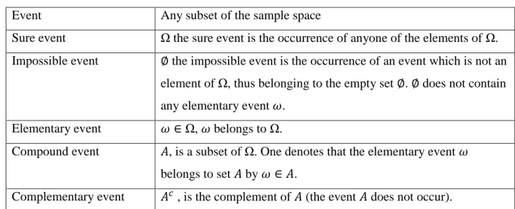
Table 1
Events and sets. Events classification.
Event Any subset of the sample space
Sure event the sure event is the occurrence of anyone of the elements of .
Impossible event the impossible event is the occurrence of an event which is not an
element of , thus belonging to the empty set . does not contain any elementary event .
Elementary event , belongs to .
Compound event , is a subset of . One denotes that the elementary event belongs to set by .
or , union of and . The union of sets and contains all the
elements which belong at least to one of the two sets.
and , intersection of and . The intersection of sets and contains all the elements which belong both to and .
and mutually
exclusive
. There is not any event common to and .
equivalent to , that can be read equals .
All these definitions are in fact quite natural. Consider again the experiment about tossing
a die, “ comes up” is an elementary event, while “I draw an even number” is a compound event. Similarly, “I draw an odd number” is the opposite event to the previous one, and “ comes up” is
an impossible event, etc. The experiment could be extended, for instance when tossing two dice: the outcome “the sum of the two faces coming up is ” is a compound event, etc.
From these basic definitions, we are now in a position to introduce the following
definitions and properties, themselves quite intuitive
.
Fig. 1
Two events are mutually exclusive if they cannot occur at the same time (i.e., they have
no common outcomes).
In probability theory, events , , ..., are said to be mutually exclusive if the occurrence of any one of them automatically implies the non-occurrence of the remaining
events. Therefore, two mutually exclusive events cannot both occur. For example, one cannot
When events are not mutually exclusive (inclusive events, i.e., non-mutually exclusive
events), the word “or” allows for the possibility of both events happening.
Events are collectively exhaustive if all the possibilities for outcomes are exhausted, and
at least one of those outcomes must occur. For example, there are theoretically only two
possibilities for flipping a coin. Flipping a head and flipping a tail are collectively exhaustive
events. Events can be both mutually exclusive and collectively exhaustive. In the case of flipping
a coin, flipping a head and flipping a tail are also mutually exclusive events. Both outcomes
cannot occur for a single trial (i.e., when a coin is flipped only once).
Entire group of events ( ):
.
Entire group of incompatible events:
; , , .
Two or more events are said to be mutually exclusive or incompatible when only one of
those events can occur at a time. No two of these events occur simultaneously, i.e. the
occurrence of one prevents the occurrence of the others.
The "Mutually Exclusivity" property gives an idea of the inter relationships between the
events, i.e. whether they are connected or not. Events which are mutually exclusive are not
connected.
Choosing an appropriate sample space
Regardless of their number, different elements of the sample space should be distinct and
mutually exclusive so that when the experiment is carried out, there is a unique outcome. For
example, the sample space associated with the roll of a die cannot contain “1 or 3” as a possible
outcome and also “1 or 4” as another possible outcome. When the roll is a 1, the outcome of the
experiment would not be unique.
A given physical situation may be modeled in several different ways, depending on the
kind of questions that we are interested in. Generally, the sample space chosen for a probabilistic
model must be collectively exhaustive, in the sense that no matter what happens in the
addition, the sample space should have enough detail to distinguish between all outcomes of
interest to the modeler, while avoiding irrelevant details.
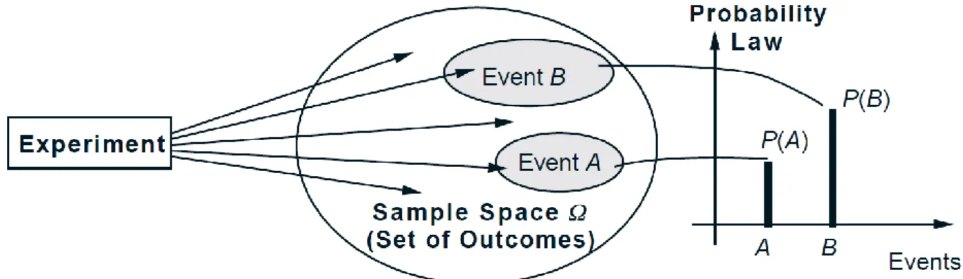
4 Probabilistic models
A probabilistic model is a mathematical description of an uncertain situation. It`s two
main ingredients are listed below and are visualized in Fig. 2.
Elements of a Probabilistic Model
The sample space , which is the set of all possible outcomes of an experiment.
The probability law, which assigns to a set of possible outcomes (an event) a nonnegative number (called the probability of ) that encodes our knowledge or
belief about the collective “likelihood” of the elements of . The probability law must
satisfy certain properties to be introduced shortly.