30 November 2000
by
Ed Greengrass
Abstract
1. Introduction...5
2. What is Information Retrieval (IR)? ...6
2.1 Definition and Terminology of Information Retrieval (IR)...6
2.1.1 Structured vs. Unstructured vs. Semi-Structured Documents ...6
2.1.2 Unstructured Documents with Structured Headers...7
2.1.3 Structure of a Document as a Document ...8
2.1.4 Goals of Information Retrieval ...8
2.1.5 Ad-Hoc Querying vs. Routing ...9
2.1.6 Evaluation of IR Performance ...9
3. Approaches to IR - General ...12
4. Classical Boolean Approach to IR...13
4.1 Automatic Generation of Boolean Queries...14
5. Extended Boolean Approach ...15
6. Vector Space Approach ...18
6.1 Building Term Vectors in Document Space ...18
6.2 Normalization of Term Vectors ...20
6.3 Classification of Term Vector Weighting Schemes...25
6.4 Computation of Similarity between Document and Query...28
6.5 Latent Semantic Indexing (LSI) — An Alternative Vector Scheme ...35
6.6 Vectors Based on n-gram Terms...41
7. Probabilistic Approach...44
7.1 What Distinguishes a Probabilistic Approach?...44
7.2 Advantages and Disadvantages of Probabilistic Approach to IR ...45
7.3 Linked Dependence ...46
7.4 Bayesian Probability Models ...47
7.4.1 Binary Independence Model ...48
7.4.2 Bayesian Inference Network Model ...52
7.4.3 Logical Imaging ...62
7.4.4 Logistic Regression...63
7.4.5 Okapi (Term Weighting Based on Two-Poisson Model) ...68
8. Routing/Classification Approaches ...71
9. Natural Language Processing (NLP) Approaches ...77
9.1 Phrase Identification and Analysis...80
9.2 Sense Disambiguation of Terms and Noun Phrases ...84
9.3 Concept Identification and Matching...87
9.3.1 Formal Concepts ...91
9.3.2 Concepts and Discourse Structure ...94
9.3.3 Proper Nouns, Complex Nominals and Discourse Structure...97
9.3.4 Integrated SFC/PN/CN Matching ...99
9.3.5 Relations and Conceptual Graph Matching ...99
9.3.6 Recognition of Semantic Similarity in CN’s ...100
9.4 Proper Noun Recognition, Categorization, Normalization, and Matching...101
9.5 Semantic Descriptions of Collections...106
9.6 Information Extraction...107
10 Clustering...111
10.2 Heuristic Cluster Methods ...116
10.3 Incremental Cluster Generation ...120
10.4 Cluster Validation ...128
11 Query Expansion and Refinement ...130
11.1 Query Expansion (Addition of Terms) ...130
11.2 Query Refinement (Term Re-Weighting)...134
11.3 Expansion/Refinement of Boolean and Other Structured Queries ...138
11.4 Re-Use of Queries...139
12 Fusion of Results ...141
12.1 Fusion of Results from Multiple Collections...141
12.2 Fusion of Results Obtained by Multiple Methods ...151
12.3 Fusion of Results Obtained by Multiple Versions of the Same Method ...160
13. User Interaction...164
13.1 Displaying and Searching Retrieved Document Sets ...164
13.2 Browsing a Document Collection...168
13.3 Interactive Directed Searching of a Collection...171
14. IR Standard - Z39.50...173
14.1 Searching via Z39.50 ...174
14.2 Retrieval via Z39.50...175
14.3 Type 102 Ranked List Query (RLQ) - A Proposed Extension to Z39.50...175
15. A Brief Review of some IR Systems ...177
15.1 LEXIS/NEXIS ...177
15.2 Dialog...178
15.3 Dow Jones News/Retrieval ...179
15.4 Topic ...179
15.5 SMART...181
15.6 INQUERY...182
16. Web-Based IR Systems...186
16.1 Web-Based Vs. Web-Accessible IR Systems...186
16.2 What a Web-Based IR Engine Must Do ...186
16.3 Web Characteristics Relevant to IR...187
16.4 Web Search Engines ...190
16.4.1 Automated Indexing on the Web ...191
16.4.4 Meta-Querying on the Web ...202
16.4.5 Personal Assistants for Web Browsing...206
1. Introduction
This report provides an overview of the state of the art in Information Retrieval (IR), both com-mercial practice and research. More specifically, it deals with the retrieval of unstructured and semi-structured text documents or messages. It doesn’t claim to be exhaustive. If it were exhaus-tive today, it wouldn’t be exhausexhaus-tive tomorrow given the dynamic nature of the field.
The report is divided into five broad areas. Area one (chapters one and two) discusses the basic concepts and definitions, e.g., what IR means, what its goals are, what entities it attempts to retrieve, the criteria by which IR systems are evaluated (and the limitations of those criteria), and how IR differs from retrieval via a traditional DBMS.
Area two (chapters three to ten) discusses each of the major approaches to the generation of que-ries and their interpretation, by Information Retrieval engines: classical boolean, extended bool-ean, vector space, probabilistic, and semantic/natural language processing (NLP). It also discusses IR “querying” from the perspective of routing and classification of an incoming stream of documents (as distinct from their retrieval from fixed collections). (In the routing context, que-ries are often called topics or classifications.) Finally, it discusses methods of clustering docu-ments within a collection as a form of unsupervised classification, and as an aid to efficient retrieval.
Area three (chapter eleven) discusses the automatic and interactive expansion and refinement of user-generated queries, e.g., on the basis of user “relevance” feedback. Additionally, it discusses the re-use of queries.
Area four (chapter twelve) discusses the “fusion” of streams of output documents resulting from multiple, parallel retrievals into a single ranked stream that can be presented to the user. Two kinds of fusion are discussed: (1) A given query may be issued to multiple document collections using a common IR method. The documents retrieved from each of those collections must be merged into a single stream, ideally the same stream that would have resulted if these separate collections had been integrated into a single collection. (2) The same query may be executed by multiple IR methods (or the same information need may be formulated as multiple queries). In this way, a single query or information need may result in multiple retrievals being applied to the same document collection, each retrieval returning a different set of documents or a different ranking of the documents retrieved. Again, the results of these multiple retrievals must be merged and ranked for presentation to the user.
Area five (chapter thirteen) discusses user interaction with IR systems, i.e., system aid in the for-mulation and refinement of queries, system display of data and retrieved results in ways that aid user understanding, user browsing of (and interaction with) displayed data and results, etc.
which reflects enhancements in IR technology, especially the ability to retrieve documents ranked by the likelihood that they satisfy the user’s information need.
Area seven (chapter fifteen) illustrates the state of the art by discussing briefly six actual IR sys-tems — four commercial and two research.
Area eight (chapter sixteen) discusses Web information retrieval, including general concepts, research approaches, and representative commercial Web IR engines.
2. What is Information Retrieval (IR)?
2.1 Definition and Terminology of Information Retrieval (IR)
The term “IR”, as used in this paper, refers to the retrieval of unstructured records, that is, records consisting primarily of free-form natural language text. Of course, other kinds of data can also be unstructured, e.g., photographic images, audio, video, etc. However, IR research has focused on retrieval of natural language text, a reasonable emphasis given the importance and immense vol-ume of textual data, on the internet and in private archives.
Some points of terminology should be clarified here. The records that IR addresses are often called “documents”. That term will be used here. IR often addresses the retrieval of documents from an organized (and relatively static) repository, most commonly called a “collection”. That term will also be used here. (The word “archive” is also used. So is the word “corpus”. The term “digital library” is becoming very common. But the generic term “collection” is still the term most commonly used in the research literature.) However, it should be understood that IR is not restricted to static collections. The collection may be a stream of messages, e.g., E-mail messages, faxes, news dispatches, flowing over the internet or some private network.
2.1.1 Structured vs. Unstructured vs. Semi-Structured Documents
iden-tify the column; an “Equipment” table in the same or a different database may also have an “age” column. Hence in general, it may be necessary to specify a path, e.g., database name, table name, column name, to uniquely identify the syntactic component to the search engine. However, the syntax of a well-structured database is such that it is always possible to specify a given syntactic component uniquely and hence it is always possible for the search engine to find all occurrences of a given component. If the given component has a definite semantics, then it is always possible for the search engine to find data with that semantics, e.g., to find the ages of all employees. By contrast, in a collection of unstructured natural language documents, there is no well-defined syntactic position where a search engine could find data with a given semantics, e.g., the ages of employees. In a random collection of documents, there is no guarantee that they are all about the same topic, e.g., employees. Even if it is known that the documents are all about employees, there is no guarantee that they all specify the age of an employee (or that any do). Even if it is known that some documents do specify the age of an employee, there is no simple well-defined way of telling where the age occurs in a given document, e.g., in what sentence or even in what para-graph. This is exactly what is meant by “unstructured;” there is no (externally) well-defined syn-tax for a given document, let alone a synsyn-tax that all the documents share. To the extent that the documents do share a syntax, there is no well-defined semantics associated with each syntactic component.
In some cases, a collection of textual documents may share a common structure and semantics, e.g., in a collection of documents containing facts about countries, each document may contain data about a different country. [CIA Fact Book] The first paragraph may contain the name, loca-tion and populaloca-tion of the country in sentences that follow a fairly consistent form. Similarly, the 2nd paragraph may list the principal industries and exports, again in sentences that follow a fairly standard form. Such a collection is called “semi-structured.” Although the data about a country does not occupy well-defined columns in a well-defined table, e.g., name, population, location, etc., as they would do in a structured database, the data nevertheless occupies fairly standard posi-tions in the text of each document with further clues, e.g., key words like “population”, that make it fairly easy to write algorithms or at least heuristics for extracting the data and storing it in struc-tured tables.
2.1.2 Unstructured Documents with Structured Headers
pub-lished after a given date. But finding documents that contain data on a particular topic is a much harder task. This task is one of the principal problems addressed by IR research.
2.1.3 Structure of a Document as a Document
IR documents are often structured in another way: They have a structure as documents. For exam-ple, a book may have a structure that consists of certain components by virtue of being a book, e.g., it contains a title page, chapters, etc. The chapters are composed of paragraphs which are composed of sentences, which are composed of words, etc. If the book is a textbook, it will typi-cally have a richer structure including a table of contents, an introduction or preface, an index, a bibliography, etc. The chapters may contain figures, graphs, photographs, tables, citations, etc. This structure may be specified explicitly by a “markup” language such as SGML or HTML. Or the structure may be implicit in the format and organization of the book. A software tool may be able to recover much of this structure by using format clues such as indentation, key words (like “Index” or “Figure”) etc., and mark up a document semi-automatically. But in all such cases, the structure is still metadata in the sense that it characterizes the organization of the document, not its semantic content. The search engine may be able to find chapter one, or section one, or figure one, easily. But finding a section dealing with a given topic, e.g., “information retrieval,” or containing the value of an attribute of some real-world entity, e.g., the date on which a given organization was incorporated, is a much more difficult and far less well-defined problem.
2.1.4 Goals of Information Retrieval
IR focuses on retrieving documents based on the content of their unstructured components. An IR request (typically called a “query”) may specify desired characteristics of both the structured and unstructured components of the documents to be retrieved, e.g., “The documents should be about ‘Information retrieval’ and their author must be ‘Smith’.” In this example, the query asks for doc-uments whose body (the unstructured part) is “about” a certain topic and whose author (a struc-tured part) has a specified value.
2.1.5 Ad-Hoc Querying vs. Routing
A distinction is often made between routing and ad-hoc querying. [TREC 3 Overview, Harman] In the latter, the user formulates any number of arbitrary queries but applies them to a fixed collec-tion. In routing, the queries are a fixed number of topics; each message in an incoming (and hence constantly changing) stream of messages is classified according to which topic it fits most closely and “routed” to the class corresponding to that topic. (In many routing experiments, there is just one topic or query; hence, there are just two classes, relevant and non-relevant.)
2.1.6 Evaluation of IR Performance
At the heart of IR evaluation is the concept of “relevance”. Relevance is an inherently subjective concept [Salton, 83, Pg 173] [Hersh, SIGIR ‘95] in the sense that satisfaction of human needs is the ultimate goal, and hence the judgment of human users as to how well retrieved documents sat-isfy their needs is the ultimate criterion of relevance. Moreover, human beings often disagree about whether a given document is relevant to a given query. [Hersh, SIGIR ‘95] Disagreement among human judges is even more likely when the question is not absolute relevance but degree of relevance. There are other complications: Relevance depends not only on the query and the col-lection but also on the context, e.g., the user’s personal needs, preferences, knowledge, expertise, language, etc. [Hersh, SIGIR ‘95] {van Rijsbergen, SIGIR ‘89] Hence, a given document retrieved by a given query for a given user may be relevant to that user on one day but not on another. {Hersh, SIGIR ‘95] Or the given document may be relevant to one user but not to another even though they both issued the same query. (This may be either because their needs are different or because they “meant” different things by the nominally “same” query.) Or the document may be relevant if retrieved from one collection but not if retrieved from another collection. Or rele-vance of a document may depend on the order of retrieval, e.g., the second document retrieved is less relevant to a given user if the first document retrieved satisfies the user’s need. In general, there is a difference between relevance to the topic of a given query and usefulness to the user who issued the given query. For this reason, some writers [Saracevic, 1997] [Korfhage, 1997] [Salton, 1983] distinguish between relevance to the user’s query, and pertinence to the user’s needs.
On the other hand, early experiments “that looked at differing relevance assessments, … found that for ‘comparative purposes’ (i.e., testing whether a certain technique is better than some other technique) any ‘reasonable’ set of relevance assessments gave the same ordering of techniques even though absolute performance scores differed.” [Voorhees, pc]
Two measures of IR success, both based on the concept of relevance [to a given query or informa-tion need], are widely used: “precision” and “recall.” Precision is defined as, “the ratio of relevant items retrieved to all items retrieved, or the probability given that an item is retrieved [that] it will be relevant.” [Saracevic, SIGIR ‘95] Recall is defined as, “the ratio of relevant items retrieved to all relevant items in a file [i.e., collection], or the probability given that an item is relevant [that] it will be retrieved.” [Saracevic, SIGIR ‘95] Other measures have been proposed, [Salton, ‘83, pps 172-186] [van Rijsbergen, 1979] but these are by far the most widely used. Note that there is an obvious trade-off here. If one retrieves all of the documents in a collection, then one is sure of retrieving all the relevant documents in the collection in which case the recall will be “perfect”, i.e., one. On the other hand, in the common situation where only a small proportion of the docu-ments in a collection are relevant to the given query, retrieving everything will give a very low precision (close to zero). The usual plausible assumption is that the user wants the best achievable combination of good precision and good recall, i.e., ideally he would like to retrieve all the rele-vant documents and no non-relerele-vant documents.
But this plausible assumption is open to some very serious objections. It is often the case that the user only wants a small subset of a (possibly large) set of relevant documents. The relevant docu-ments may contain a lot of redundancy; a few of them may be sufficient to tell the user everything he wants to know {Hersh, SIGIR ‘95]. Or the user may be looking for evidence to support a hypothesis or to reduce uncertainty about the hypothesis; a few documents may provide sufficient evidence for that purpose. [Florance, SIGIR ‘95] Or the user may only want the most up-to-date documents on a given topic, e.g., for a lawyer the latest legal opinion or statute may have super-seded earlier precedents or statutes.[Turtle, SIGIR ‘94] In general, it is often the case that there are multiple subsets of relevant documents such that any one of these subsets will satisfy the user’s requirement, rather than a single unique set of the relevant documents. On the other hand, two relevant documents may present contradictory views of some issue of concern to the user; hence, the user may be seriously misled if he only sees some of the relevant documents.
In practice, some users attach greater importance to precision, i.e., they want to see some relevant documents without wading through a lot of junk. Others attach greater importance to recall, i.e., they want to see the highest possible proportion of relevant documents. Hence, van Rijsbergen [1979] offers the E (for Effectiveness) measure, which allows one to specify the relative impor-tance of precision and recall:
where P is precision, R is recall, andα is a parameter which varies from zero (user attaches no importance to precision), through one half (user attaches equal importance to precision and recall), to one (user attaches no importance to recall).
Measuring precision is (relatively) easy; if a set of competent users or judges agree on the rele-vance or non-relerele-vance of each of the retrieved documents, then calculating the precision is straightforward. Of course, this assumes that the set of retrieved documents is of manageable size, as it must be if it is to be of value to the user. If the retrieved documents are ranked, one can
E 1 1
α 1
P
---
(1–α)1 R ---+
---–
always reduce the size of the retrieved set by setting the threshold higher, e.g., only look at the top 100, or the top 20. Measuring recall is much more difficult because it depends on knowing the number of relevant documents in the entire collection, which means that all the documents in the entire collection must be assessed. [Saracevic, SIGIR ‘95] If the collection is large, this is not fea-sible. (The Text REtrieval, i.e., TREC, Conferences attempt to circumvent the problem by pooling samples, e.g., the top 100 documents, retrieved by each competing IR engine; the assumption is made that every relevant document is being retrieved by at least one of the competitors. [Harman, TREC 3 Overview, TREC 4] This works better for comparing engines than for computing an absolute measure of recall.)
Most of the IR systems discussed in this report return an ordered list of document, i.e., the docu-ments are ranked according to some measure, often statistical or probabilistic, of the likelihood that they are relevant to the user’s request. The usual assumption is that the user will start with the first document (or some surrogate like a title or summary), the document the system estimates as “best,” and work her way down the list until her needs have been satisfied, or her patience exhausted. (But see some alternatives discussed under User Interaction.) Hence, another measure of system effectiveness is how many non-relevant documents the user has to examine before reaching the number of relevant documents she needs or desires. If the system returns 20 docu-ments, and only three are relevant, the precision is 3/20 or 0.15. However, as a practical matter, it makes a considerable difference to the user whether the three relevant documents are the first three in the ordered list (she doesn’t have to look at any non-relevant documents if those three sat-isfy her need), or the last three (she has to look at 17 non-relevant documents before she reaches the “good stuff.”) Typically, the situation will be intermediate, e.g., the three relevant documents may appear at positions (ranks) four, seven, and 15. To complicate matters further, it is entirely possible that several documents will be tied according to the given systems measure, e.g., relevant document four and non-relevant documents five and six may receive the same probability of rele-vance value; in that case, the order of those three documents is arbitrary, i.e., it is equally likely that the relevant document will occupy positions four, five, or six. Hence, Cooper [JASIS, 1968] has proposed the “Expected Search Length (ESL)” for a given query q, a measure of the number of non-relevant documents the user will have to wade through to reach a specified number of rele-vant documents; Cooper’s measure takes into account the uncertainty produced by ties.
Another common variation on average precision is the eleven-point average precision. The preci-sion is calculated for recalls (in practice, estimated recalls) of zero, 0.1, 0.2,...,1.0. Then, these 11 precisions, computed for uniformly spaced values of recall, are averaged.
3. Approaches to IR - General
Broadly, there are two major categories of IR technology and research: semantic and statistical. Semantic approaches attempt to implement some degree of syntactic and semantic analysis; in other words, they try to reproduce to some (perhaps modest) degree the understanding of the nat-ural language text that a human user would provide. In statistical approaches, the documents that are retrieved or that are highly ranked are those that match the query most closely in terms of some statistical measure. By far the greatest amount of work to date has been devoted to statistical approaches so these will be discussed first. (Indeed, even semantic approaches almost always use, or are used in conjunction with, statistical methods. This is discussed in detail later.)
Statistical approaches fall into a number of categories: boolean, extended boolean, vector space, and probabilistic. Statistical approaches break documents and queries into terms. These terms are the population that is counted and measured statistically. Most commonly, the terms are words that occur in a given query or collection of documents. The words often undergo pre-processing. They are “stemmed” to extract the “root” of each word. [Porter, Program, 1980] [Porter, Read-ings, 1997] The objective is to eliminate the variation that arises from the occurrence of different grammatical forms of the same word, e.g., “retrieve,” “retrieved,” “retrieves,” and “retrieval” should all be recognized as forms of the same word. Hence, it should not be necessary for the user who formulates a query to specify every possible form of a word that he believes may occur in the documents for which he is searching. Another common form of preprocessing is the elimination of common words that have little power to discriminate relevant from non-relevant documents, e.g., “the”, “a”, “it” and the like. Hence, IR engines are usually provided with a “stop list” of such “noise” words. Note that both stemming and stop lists are language-dependent.
Some sophisticated engines also extract “phrases” as terms. A phrase is a combination of adjacent words which may be recognized by frequency of co-occurrence in a given collection or by pres-ence in a phrase dictionary.
be language-independent, and has even been used to sort documents by language, or by topic within language. For similar reasons, n-gram statistics appear to be relatively insensitive to degraded text, e.g., spelling errors, typos, errors due to poor print quality in OCR transmission, etc. [Pearce et al., 1996]
Numeric weights are commonly assigned to document and query terms. A weight is assigned to a given term within a given document, i.e., the same term may have a different weight in each dis-tinct document in which it occurs. The weight is usually a measure of how effective the given term is likely to be in distinguishing the given document from other documents in the given collection. The weight is often normalized to be a fraction between zero and one. Weights can also be assigned to the terms in a query. The weight of a query term is usually a measure of how much importance the term is to be assigned in computation of the similarity of documents to the given query. As with documents, a given term may have a different weight in one query than in another. Query term weights are also usually normalized to be fractions between zero and one.
4. Classical Boolean Approach to IR
In the boolean case, the query is formulated as a boolean combination of terms. A conventional boolean query uses the classical operators AND, OR, and NOT. The query “t1AND t2” is satisfied by a given document D1 if and only if D1 contains both terms t1 and t2. Similarly, the query “t1 OR t2” is satisfied by D1if and only if it contains t1or t2or both. The query “t1AND NOT t2” sat-isfies D1if and only if it contains t1and does not contain t2. More complex boolean queries can be built up out of these operators and evaluated according to the classical rules of boolean algebra. Such a classical boolean query is either true or false. Correspondingly, a document either satisfies such a query (is “relevant”) or does not satisfy it (is non-relevant”). No ranking is possible, a sig-nificant limitation. [Harman, JASIS, 1992] Note however that if stemming is employed, a query condition specifying that a document must contain the word “retrieve” will be satisfied by a docu-ment that contains any of the forms “retrieve”, “retrieves”, “retrieved”, “retrieval”, etc.
Several kinds of refinement of this classical boolean query are possible when it is applied to IR. First, the query may be applied to a specified syntactic component of each document, e.g., the boolean condition may be applied to the title or the abstract rather than to the document as a whole.
proximity operator may specify order as well as proximity, e.g., not only how close two words must be but in what order they must occur.
The classical boolean approach does not use term weights. Or, what comes to the same thing, it uses only two weights, zero (a term is absent) and one (a term is present).
The classical boolean model can be viewed as a crude way of expressing phrase and thesaurus relationships. For example, t1AND t2 says that both terms t1 and t2must be present, a condition that is applicable if the two terms form a phrase. If a proximity operator is employed, the boolean condition can be made to say that t2 must immediately follow t1 in the text, which corresponds still more closely (though still crudely) to the conventional meaning of a “phrase.” Similarly, t1 OR t2says that either t1or t2can serve as an index term to relevant documents, i.e., in some sense t1 and t2are “equivalent”. This is roughly speaking what we mean when we assign t1and t2 to the same class in a thesaurus. In fact, some systems use this viewpoint to generate expanded bool-ean conditions automatically, e.g., given a set of query terms supplied by the user, “a boolbool-ean expression is composed by ORing each … query term with any stored synonyms and then AND-ing these clusters together.” [Anick, SIGIR ‘94]
4.1 Automatic Generation of Boolean Queries
The logical structure of Boolean queries, which is their greatest virtue, is also one of their most serious drawbacks. Non-mathematical or novice users often experience difficulty in formulating Boolean queries.[Harman, JASIS, 1992] Indeed, they often misinterpret the meaning of the AND and OR operators. (In particular, they often use “AND,” set intersection, when “OR,” set union, is intended.) [Ogden & Kaplan, cited in Ogden & Bernick, 1997] This has led to schemes for auto-matic generation of Boolean queries. [Anick, SIGIR’94] [Salton, IP&M, 1988]
In the Anick approach mentioned above, the query terms (presumably after stemming, removing stop words, etc.) are Ored together. Each OR term is expanded with any synonyms from an on-line thesaurus. The Salton approach, by contrast, imposes a Boolean structure on the terms sup-plied by the user. No thesaurus is employed.
Salton starts with a natural language query. The usual stemming and removal of stop words gener-ates a set of user terms, which are ORed together as in the Anick approach. However, Salton then looks for pairs (and triples) of these user-supplied terms that co-occur in one or more documents. Since two or three of these user terms might occur in the same document by chance, Salton then uses a formula for pairwise correlation to determine if any given pair of co-occurring terms Tiand Tj co-occur more frequently than would be expected by chance alone. A similar correlation for-mula is used for co-occurring triples, i.e., three of the user-supplied words occurring in the same document. Each pair or triple whose computed correlation exceeds a pre-determined threshold is then grouped with a Boolean AND, e.g., if the pair ti, tjand the triple tl, tm, tn exceed the thresh-old, then the automatically generated Boolean query (assuming t terms) becomes:
It should be stressed again that the pairs are triples are drawn entirely from the terms originally supplied by the user; no thesaurus-based expansion as with Anick, and no query expansion based on relevance feedback (see below) is employed. However, combining these various techniques is certainly feasible.
As a further refinement, Salton ranks the terms (single terms, pairs, and triples) in the automati-cally generated Boolean expression in descending order by inverse document frequency. (See below for a definition of idf. High-idf terms tend to be better discriminators of relevance than low-idf terms.) He can estimate the number of documents that a given term (or pair or triple) will be responsible for retrieving from its frequency of occurrence in documents. If the total estimated number of documents that will be retrieved by the Boolean query exceeds the number of docu-ments that the user wants to see, he can reduce the estimated number by deleting OR terms from the query starting with those that have the lowest idf ranking. This gives the user, not a true rele-vance ranking of documents, but at least some control over the number retrieved, something that ordinary Boolean retrieval does not provide.
5. Extended Boolean Approach
Even with the addition of a proximity operator, boolean conditions remain classical in the sense that they are either true or false. Such an all-or-nothing condition tends to have the effect that either an intimidatingly large number of documents or none at all are retrieved. [Harman, JASIS, 1992] Classical Boolean models also tend to produce counter-intuitive results because of this all-or-nothing characteristic, e.g., in response to a multi-term OR, “a document containing all [or many of] the query terms is not treated better than a document containing one term.” [Salton et al., IP&M, 1988] Similarly, in response to a multi-term AND, “[A] document containing all but one query term is treated just as badly as a document containing no query term at all.” [Salton et al., IP&M, 1988] A number of extended boolean models have been developed to provide ranked out-put, i.e., provide output such that some documents satisfy the query condition more closely than others. [Lee, SIGIR ‘94] These extended boolean models employ extended boolean operators (also called “soft boolean” operators).
Given a query consisting of n query terms t1, t2, …, tn, with corresponding weights wq1, wq2, …, wqn, and a document D, with corresponding weights wd1, wd2, …, wdnfor the same n terms, the p-norm model defines similarity functions for the extended boolean AND and extended boolean OR of the n terms. The extended boolean AND function computes the similarity of the given docu-ment with a query that ANDs the given terms together. Similarly, the extended boolean OR func-tion computes the similarity of the given document with a query that ORs the given terms together. Each similarity is computed as a number in the closed interval [0, 1]. More elaborate boolean queries can obviously be composed from the AND and OR functions. The extended bool-ean functions for the p-norm model are given by:
and
The p-norm model has a parameter that can be used to “tune” the model; most of the other models studied by Lee also have such a parameter, though the effect and interpretation of the parameter varies with the model. The parameter p in the p-norm model can vary from one to infinity and has a very clear interpretation. At p= infinity, the p-norm model is equivalent to the classical boolean model; AND corresponds to strict phrase assignment (i.e., all the components of the phrase must be present for the AND to evaluate to non-zero), OR to strict thesaurus class assignment (i.e., presence of any one member of the class is sufficient for the OR to evaluate to one; there is no additional score if two or more are present.). At low to moderate p, e.g., between 2 and 5, AND corresponds to loose phrase assignment, i.e., “the presence of all phrase components is worth more than the presence of only some of the components; terms are not compulsory.” That is, the p-norm AND generalizes the strict boolean AND in the sense that a single low-weighted term substantially lowers the total similarity score, even if all the other terms have high weights. On the other hand, the p-norm AND differs from the strict boolean AND because a single zero weighted, i.e., missing, term does not reduce the total similarity score to zero. Similarly, at low to moderate p, OR corresponds to loose thesaurus class assignment, i.e., “the presence of several terms from a class is worth more than the presence of only one term.” In other words, the p-norm OR general-izes the strict boolean OR in the sense that a single high-weighted term can produce a fairly high total similarity score even if all the other terms are low-weighted or missing (zero weighted). On the other hand, the p-norm OR differs from the strict boolean OR because a single high-weighted term is not enough to maximize the similarity score; additional non-zero terms will increase the total score to some degree. At p = 1, the p-norm model reduces to the pure “vector space” model which is discussed in the next section, i.e., “terms are independent of each other; distinction between phrase and thesaurus assignment disappears.” In fact, at p = 1, AND and OR become identical. [Salton, et al., CACM 1983] They both become identical to cosine similarity, discussed in the next section.
SIMAND(d t,( ,1wq1)AND…AND t( ,nwqn)) 1
1–wdi
( )p
wqi p
•
( )
i=1 n
∑
wqi p i=1
n
∑
--- ---1p
–
= ,(1≤ ≤p ∞)
SIMOR(d t,( ,1wq1)OR…OR t( ,nwqn))
wdi p wqi p • ( )
i=1 n
∑
wqi p i=1
n
∑
--- ---1p
The classical boolean operators AND and OR are binary, i.e., they connect two terms. However, they are also associative, i.e., t1AND (t2AND t3) is equivalent to (t1AND t2) AND t3. This is not true for the p-norm model (and some of the other extended boolean models). The p-norm model (and the other models with the same problem) circumvent this difficulty by defining the extended boolean operators as n-ary, i.e., connecting n terms, rather than binary. So the above boolean expression becomes AND (t1, t2, t3). {Lee, SIGIR ‘94] This expression is true if and only if all three terms are present.
The p-norm model supports assignment of weights to the query terms as well as the document terms. The p-norm formulas extend to this case in a quite straightforward manner. The weights are relative rather than absolute, e.g., the query (t1, 1) AND (t2, 1) with a weight of one assigned to each term is exactly equivalent to the query (t1, 0.1) AND (t2, 0.1) with a weight of 0.1 assigned to each term. This is so because the p-norm formulas normalize the query weights. Relative weights are easier and more natural for the user to assign than absolute weights. It is easier for a user to say that t1 is more important (or even twice as important) than t2 than to say exactly how impor-tant either term is. {Lee, SIGIR ‘94]
A further degree of flexibility can be achieved in the p-norm model by permitting the user to assign a different value of p to each boolean operator in a given boolean expression. This allows the user to say, e.g., that a strict phrase interpretation should be given to one AND in the given expression, a looser interpretation to another AND in the same expression, etc. {Salton et al., CACM 1983]
What makes the p-norm model superior to the alternatives surveyed by Lee? Its primary advan-tage is that it gives equal importance to all its operands.This does not mean that it ignores docu-ment and term weights. On the contrary, the docudocu-ment weights (assigned typically by the program that indexes the document collection), and the query weights (assigned typically by the user who formulates the query, although automatic modification of these weights is discussed in a later sec-tion), are essential elements of the p-norm functions as given above. What “equal importance” means is that the p-norm functions evaluate all term weights in the same way; they do not give special importance to certain terms on the basis of their ordinal positions, i.e., any permutation of term order is equivalent to any other. Moreover, p-norm does not give special importance to the terms with minimum or maximum weights, to the exclusion of other terms. For example, one or two high-weighted query terms in a given document will yield a high (relatively close to 1) value of a p-norm OR for the given document relative to the given query. It doesn’t matter in the least which terms are highly weighted. Moreover, if other query terms are also present in the given doc-ument, they will add to the value of the OR even if they have neither the maximum nor the mini-mum weight in the set of query terms matching the given document (“match” terms).
A probabilistic form of extended boolean has been developed [Greiff, SIGIR ‘97] in which a probabilistic OR is computed in terms of the probability of its component terms, and similarly for AND. See section on “Bayesian Inference Network Model” for further details.
Experiments have shown that the extended boolean model can achieve greater IR performance than either the classical boolean or the vector space model. But there is a price. Formulating effec-tive extended boolean queries obviously involves more thought and expertise in the query domain than formulating either a classical boolean query, or a simple set of terms with or without weights as in the vector space model.
6. Vector Space Approach
6.1 Building Term Vectors in Document Space
One common approach to document representation and indexing for statistical purposes is to rep-resent each textual document as a set of terms. Most commonly, the terms are words extracted automatically from the documents themselves, although they may also be phrases, n-grams, or, manually assigned descriptor terms. (of course, any such term-based representation sacrifices information about the order in which the terms occur in the document, syntactic information, etc.) Often, if the terms are words extracted from the documents, “stop” words (i.e., “noise” words with little discriminatory power) are eliminated, and the remaining words are stemmed so that only one grammatical form (or the stem common to all the forms) of a given word or phrase remains. (Stop lists and stemming can sometimes be avoided if the terms are n-grams — see dis-cussion below.) We can apply this process to each document in a given collection, generating a set of terms that represents the given document. If we then take the union of all these sets of terms, we obtain the set of terms that represents the entire collection. This set of terms defines a “space” such that each distinct term represents one dimension in that space. Since we are representing each document as a set of terms, we can view this space as a “document space”. [Salton, 1983] [Salton, 1989]
We can then assign a numeric weight to each term in a given document, representing an estimate (usually but not necessarily statistical) of the usefulness of the given term as a descriptor of the given document, i.e., an estimate of its usefulness for distinguishing the given document from other documents in the same collection. It should be stressed that a given term may receive a dif-ferent weight in each document in which it occurs; a term may be a better descriptor of one docu-ment than of another. A term that is not in a given docudocu-ment receives a weight of zero in that document. The weights assigned to the terms in a given document D1 can then be interpreted as the coordinates of D1in the document space; in other words, D1is represented as a point in docu-ment space. Equivalently, we can interpret D1as a vector from the origin of document space to the point defined by D1’s coordinates.
We can combine the “document space” and “term space” perspectives by viewing the collection as represented by a document-by-term matrix. Each row of this matrix is a document (in term space). Each column of this matrix is a term (in document space). The element at row i, column j, is the weight of term j in document i.
A query may be specified by the user as a set of terms with accompanying numeric weights. Or a query may be specified in natural language. In the latter case, the query can be processed exactly like a document; indeed, the query might be a document, e.g., a sample of the kind of document the user wants to retrieve. A natural language query can receive the usual processing, i.e., removal of “stop” words, stemming, etc., transforming it into a set of terms with accompanying weights. (Again, stoplists and stemming are not applicable if the queries and terms are described using n-gram terms.) Hence, the query can always be interpreted as another document in document space. Note: if the query contains terms that are not in the collection, these represent additional dimen-sions in document space.
An important question is how weights are assigned to terms either in documents or in queries. A variety of weighting schemes have been used. Given a large collection, manual assignment of weights is very expensive. The most successful and widely used scheme for automatic generation of weights is the “term frequency * inverse document frequency” weighting scheme, commonly abbreviated “tf*idf”. The “term frequency” (tf) is the frequency of occurrence of the given term within the given document. Hence, tf is a document-specific statistic; it varies from one document to another, attempting to measure the importance of the term within a given document. By con-trast, inverse document frequency (idf) is a “global” statistic; idf characterizes a given term within an entire collection of documents. It is a measure of how widely the term is distributed over the given collection, and hence of how likely the term is to occur within any given document by chance. The idf is defined as “ln (N/n)” where N is the number of documents in the collection and n is the number of documents that contain the given term. Hence, the fewer the documents con-taining the given term, the larger the idf. If every document in the collection contains the given term, the idf is zero. This expresses the commonsense intuition that a term that occurs in every document in a given collection is not likely to be useful for distinguishing relevant from non-rele-vant documents. Or what is equivalent, a term that occurs in every document in a collection is not likely to be useful for distinguishing documents about one topic from documents about another topic. To cite a commonly-used example, in a collection of documents about computer science or software, the term “computer” is likely to occur in all or most of the documents, so it won’t be very good at discriminating documents relevant to a given query from documents that are non-rel-evant to the given query. (But the same term might be very good at discriminating a document about computer science from documents that are not about computer science in another collection where computer science documents are rare.)
infre-quently in any document (low-frequency documents), and terms that occur in most or all of the documents (high frequency documents).
6.2 Normalization of Term Vectors
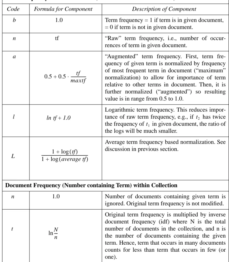
To allow for variation in document size, the weight is usually “normalized”. Two kinds of normal-ization are often applied. [Lee, SIGIR ‘95] The first is normalnormal-ization of the term frequency, “tf”. The tf is divided by the “maximum term frequency,” tfmax. The “maximum term frequency” is the frequency of the term that occurs most frequently in the given document. So the effect of izing term frequency is to generate a factor that varies between zero and one. This kind of normal-ization has been called “maximum normalnormal-ization” for obvious reasons. A variation is the formula 0.5 + (0.5*(tf/tfmax)) which causes the normalized tf to vary between 0.5 and 1. In this form, the normalization has been called “augmented normalized term frequency”. The purpose and effect of term frequency normalization (in either form) is that the weight (the “importance”) of a term in a given document should depend on its frequency of occurrence relative to other terms in the same document, not its absolute frequency of occurrence. Weighting a term by absolute frequency would obviously tend to favor longer documents over shorter documents.
However, there is a potential flaw in “maximum normalization.” The normalization factor for a given document depends only on the frequency of the most frequent term(s) in the document. Consider a document D1in which most of the terms occur with frequencies in proportion to their importance in discriminating the document’s primary topic. Now suppose that one term has a dis-proportionately high frequency, e.g., important terms t1, t2, and t3each occur twice in D1but for some stylistic reason equally important term t4occurs six times, the maximum for any term in D1. Then the frequency of t4will drag down the weights of terms t1, t2, and t3 by a factor of three in D1relative to their weights in some other similar document D2in which t1, t2, t3, and t4have equal frequencies. (The same problem arises with the “augmented normalized term frequency” but to a less extreme degree since the high frequency term will have a weight of one as with maximum normalization but it cannot drag the weights of the other terms below 0.5.)
A commonly-used alternative to normalizing the term frequency is to take its natural log plus a constant, e.g., “log (tf) + 1.” This technique, called “logarithmic term frequency,” doesn’t explic-itly take document length or maximum term frequency into account but it does “reduce the impor-tance of raw term frequency in those collections with widely varying document length.” It also reduces the effect of a term with an unusually high term frequency within a given document. In general, it reduces the effect of all variation in term frequency, since for any two term frequencies, tf1 and tf2 > 0 such that tf2 > tf1:
The second kind of normalization is by vector length. After all of the tf*idf term weights for a given document, i.e., all the components of the document vector, have been calculated, every
tf2
( )
log +1 tf1
( )
log +1 --- tf2
tf1
component of the vector is divided by the Euclidean length of the vector. The Euclidean length of the vector is the square root of the sum of the squares of all its components. Dividing each compo-nent by the Euclidean length of the vector is called “cosine” normalization because the normal-ized vector has unit length and its projection on any axis in document space is the cosine of the angle between the vector and the given axis.
Augmented maximum (term frequency) normalization and cosine normalization can be used sep-arately or together.
Cosine normalization reduces the problem (described above) of vector component weights for a given document being distorted by a single term with unusually high frequency. (But see the dis-cussion below of pivoted unique normalization which further addresses the problem.) The nor-malization factor (vector length) is a function of all the vector components so the effect of a single term with a disproportionately high frequency is diluted by the weights of all the other terms. Fur-thermore, the normalization factor is a function of each tf*idf term weight, not just the tf factor of that weight. So, the weight of a high frequency term may also be lessened by its idf factor.
However, as Lee has pointed out, situations exist in which maximum normalization may actually do better than cosine normalization. Consider a case where document D1deals with topic TAand contains a set of terms relevant to TA. Now consider document D2 which deals with TA and also deals with several other topics TB, TC, etc. Suppose that D2contains all the terms that D1contains, i.e., terms relevant to TA, but also contains many other terms relevant to TB, TC, etc. Since cosine normalization of a given document takes into account the weights of all its terms, the effect is that the weights of the terms relevant to TAwill be dragged down in D2(relative to the weights of the same terms in D1) by the weights of the terms relevant to TB, TC, etc. As a result, a user trying to retrieve documents relevant to TA will be much more likely to retrieve D1 than D2 even if they both cover TAto the same extent. Maximum normalization will do better in this case provided that the maximum frequency term relevant to TAin D2is about as frequent as the maximum frequency term in D2relevant to any of the other topics. In that case, none of the other topics will drag down the weights of TA’s terms in D2. Lee concludes that in some cases, better precision and recall can be achieved by using each normalization scheme for retrieval separately and then merging the results of the two retrieval runs. (Merging retrieval runs is discussed further below.)
“crossover” document length for which the two probability curves intersect, i.e., a document length for which the probability of relevance equals the probability of retrieval.
These observations led Singhal et al. to develop a “correction factor”, a function of document length that maps a conventional “old” document length normalization function, e.g., cosine nor-malization, into a “new” document normalization function. The correction factor rotates the old normalization function clockwise around the crossover point so that normalization values corre-sponding to document lengths below the crossover point are greater than before (so that the prob-ability of retrieval for these documents is decreased), and normalization values corresponding to document lengths above the crossover point are less than before (so that the probability of retrieval for these documents is increased). (Remember that term weights for a given document are divided by the normalization factor.) The crossover point is called the “pivot”. Hence, the new normalization function is called “pivoted normalization.”
Note that since the pivoted normalization method described below is based on correcting the doc-ument normalization so that the distribution of probability of retrieval coincides more closely with the probability of relevance (as a function of document length), this weighting method could legit-imately be called “probabilistic”. However, it differs from the probabilistic methods discussed below in section 7, because the probability distributions have been determined experimentally, by observing actual TREC collections, rather than being derived from a theoretical model.
The pivoted normalization is easily derived. Before the normalization is corrected, i.e., pivoted, the relation between new normalization and old normalization is:
new normalization = old normalization
This is a straight line with slope one through the origin of a graph, with a new normalization ver-tical axis, and an old normalization horizontal axis. This line is rotated clockwise around the pivot, i.e., around the normalization value corresponding to the crossover document length. Call this value “pivot.” After the rotation, the form of the new line (by elementary analytic geometry) is:
where the slope of the new line is less than one and K is a constant. (Note that although the old normalization function, e.g., cosine normalization, is not a linear function of term weights, the new normalization is a linear function of the old normalization.) K is evaluated by recognizing that since the line was rotated around the pivot point, new normalization equals old normalization at the pivot point. Hence, substitute pivot for both new normalization and old normalization in the
above linear equation, solve for K and then substitute this value of K back into the equation. The result (with new normalization now called pivoted normalization) is:
where slope and pivot are constant parameters for a given collection and query set. Since the rank-ing of documents in a given collection for a given query set is not affected if the normalization factor for every document is multiplied (or divided) by the same constant, these two parameters can be reduced to one by dividing the above normalization function by the constant (1.0-slope)*pivot. Singhal et al. found that the optimum value of this parameter was surprisingly close to constant across a variety of TREC sub-collections. Hence, an optimum parameter value learned from training experiments on one collection could be used to compute normalization factors for other collections.
Singhal et al. also examined closely the role of term frequencies and term frequency normaliza-tion in term weighting schemes. First, they found (by studying the above experiments) that though, as noted above, cosine normalization favors short documents over long ones, it also favors extremely long documents. This phenomenon is magnified by pivoted normalization. Further, they noted that term frequency is not an important factor in either cosine normalization or docu-ment retrieval. This is because (1) the majority of terms in a docudocu-ment only occur once, and (2) log(tf) + 1 is commonly used in place of raw term frequency, which has a “dampening effect” for tf > 1. Hence, the cosine normalization factor for a given document will be approximately equal to the square root of the number of unique terms in the given document, i.e., it increases less than linearly with number of unique terms. But document retrieval is generally governed by the num-ber of term matches between document and query, and hence making the usual simplifying assumption that occurrence of a given term in a given document is independent of the occurrence of any other term, the probability of a match between query and document varies linearly with the number of unique terms. The purpose of the document normalization is to adjust the term weights for each document so that the probability of retrieving a long document with a given query is the same as the probability of retrieving a short document. The conclusion is that cosine normaliza-tion reduces term weights by too little for very large documents. Singhal et al. propose to remedy this situation by replacing the cosine normalization value, i.e., the old normalization, by # of unique terms, in the pivoted normalization function.
Singhal et al. argue further that maximum normalization, i.e., tf/tfmax, is not the optimum method of normalizing term frequency because what matters is the frequency of the term relative to the frequencies of all the other descriptor terms, not just relative to the frequency of the most fre-quently occurring term. Hence, they propose using the function:
pivoted normalization = slope•old normalization+(1.0–slope)•pivot
---for normalized term frequency. This function has the property that its value is one ---for a term whose frequency is average for the given document, greater than one for terms whose frequencies are greater than average, and less than one for terms whose frequency is less than average.
Hence, Singhal et al. propose weighting each term in a document by the above term frequency normalization function divided by the pivoted normalization, i.e.,
Note that the idf is absent from this weighting function. This is because, for reasons explained in the next section, the idf is normally used as a factor in the weights of query terms rather than doc-ument terms. That is, if a given term occurs in a query and also in some docdoc-uments in the collec-tion being queried, the idf will be used as a factor in the weight of that term in the query vector rather than in the corresponding document vectors.
Singhal et al. tested this improved term weighting function against a set of TREC sub-collections and found that for optimum parameter values, it performed substantially better than the more familiar product of tf/tfmax and 1/cosine normalization.
It should be noted that this improved weighting scheme compensates for both of the problems noted by Lee. The effect of a term with a disproportionately high frequency in a given document is greatly reduced by the new term frequency normalization function, partly because the fre-quency of the given term is divided by the average term frefre-quency rather than the maximum term frequency, and partly because both the given term frequency and the average term frequency are replaced by their logs. The advantage of a short document dealing entirely with a topic relevant to a given query, over a longer document dealing with the relevant topic and several nonrelevant top-ics, is compensated by pivoted normalization which reduces the probability of retrieval of short documents and increases the probability of retrieval of long documents.
All of the normalization schemes discussed above (and in the following section) are based on one underlying assumption: that document relevance is independent of document length. Relevance is assumed to be wholly about how much a given document is about a given topic. Variation of doc-ument length is viewed as a complication in computing docdoc-ument relevance. Hence, all of the nor-malization schemes are aimed at factoring out the effects of document length.
If document D2is longer than document D1, relevance computation is assumed to be distorted in one of two ways. If D2is largely or entirely about the same topic Tias D1, then relevance is dis-torted by the fact that terms characteristic of the given topic will tend to occur with greater fre-quency in D2. If D2 is about a number of different topics, Ti, Tj, Tk, etc., and only a small part of D2 is about the same topic Tias D1, then the material about the other topics dilutes the effect of the relevant material, making D2 seem less relevant to TI than D1, even though both documents may contain the same information about Ti. Normalization is largely aimed at overcoming these two kinds of distortion.
1+log( )tf 1+log(average tf)
---Completely ignored is a third possibility: that the user actually prefers either short or long docu-ments about Ti. If the user prefers the longer document, D2, e.g., she needs all the details it pro-vides, then D2 is more relevant to Tirelative the users needs. Or to use a term that may be more appropriate, D2may be more pertinent or more useful to the user in meeting her present informa-tion need, as expressed by Ti. Of course, D1may be more useful; perhaps the user needs a concise summary of the main facts or ideas about Ti, and has neither time nor need for a more detailed exposition. In either case, document size is an important parameter in computing the documents relevance for purposes of selection and ranking in the retrieval set returned to the user. This indi-cates that either the document and topic vectors should not be normalized, or that the document size should enter explicitly into the document topic similarity computation. This issue is discussed further in section 6.4, which discusses document-topic similarity functions.
6.3 Classification of Term Vector Weighting Schemes
Since the various alternatives discussed above for computing and normalizing term weights can be (and have been) used in a variety of combinations, a conventional code scheme (associated with a popular IR research engine called the SMART system) has been defined and widely adopted to classify the alternatives. [Salton, IP&M, 1988] [Lee, SIGIR ‘95] See Table 1.
Table 1: Components of schemes for weighting given term in given document
Term Frequency within Document (Unnormalized or Normalized)
Code Formula for Component Description of Component
b 1.0 Term frequency = 1 if term is in given document, = 0 if term is not in given document.
n tf “Raw” term frequency, i.e., number of occur-rences of term in given document.
a “Augmented” term frequency. First, term fre-quency of given term is normalized by frefre-quency of most frequent term in document (“maximum” normalization) to allow for importance of term relative to other terms in document. Then, it is further normalized (“augmented”) so resulting value is in range from 0.5 to 1.0.
l
Logarithmic term frequency. This reduces impor-tance of raw term frequency, e.g., if has twice the frequency of in given document, the ratio of the logs will be much smaller.
L
Average term frequency based normalization. See discussion in previous section.
Document Frequency (Number containing Term) within Collection
n 1.0 Number of documents containing given term is ignored. Original term frequency is not modified.
t
Original term frequency is multiplied by inverse document frequency (idf) where N is the total number of documents in the collection, and n is the number of documents containing the given term. Hence, term that occurs in many documents counts for less than term that occurs in few (or one).
0.5 0.5 tf maxtf
---⋅
+
ln tf+1.0 t2
t1
1+log( )tf 1+log(average tf)
measures term frequency within the query, and the document length factor normalizes for query length. Only the idf factor in the weight of a query term is a measure of the distribution in the col-lection being queried, not in the query itself.) This scheme has exhibited high retrieval effective-ness for the Text REtrieval Conference (TREC) query sets and collections. [Lee, SIGIR ‘95] However, Lnu-ltc weighting exhibited even better effectiveness against TREC3 and TREC 4 query sets and collections. [Singhal et al., SIGIR ‘96] [Buckley et al., TREC 4]
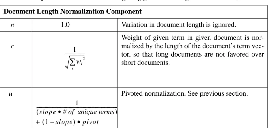
The weighting scheme classification described above is open-ended. Indeed, the SMART team, originators of this classification, have only recently added the L option to the term frequency fac-tor, and the u option to the document length normalization factor.
Note that although the idf of a given term is a statistic that characterizes that term relative to a given collection of documents, not relative to a query, it is common to use the idf to weight the occurrence of the given term in queries being applied to the collection, not to weight its occur-rence in the document vectors that describe the collection itself. The lnc-ltc and Lnu-Ltu weight-ing schemes are examples. There are simple reasons for this. First, it is more efficient for purposes of collection maintenance. Whenever new documents are added to the collection (or old ments are removed), the idf must be recomputed for each descriptor term in the affected docu-ments. It would be inefficient to recompute the weight of such a term in every document in which it occurs. Moreover, it is unnecessary for the purposes of a query/document similarity calculation, since the document ranking produced for a given query will be exactly the same whether the idf’s enter the computation as factors in the query term weights, or factors in the document term weights, or both.
In a weighting scheme like tf*idf, the normalized term frequency of a given term in a given docu-ment is multiplied by its idf so that “good” descriptor terms (which characterize only a relatively small number of documents in a given collection) are weighted more heavily than “bad” descrip-tor terms (which are so common that they occur in a great many documents in the given collec-tion, and hence are of little value in discriminating between relevant and non-relevant documents).
Document Length Normalization Component
n 1.0 Variation in document length is ignored.
c
Weight of given term in given document is nor-malized by the length of the document’s term vec-tor, so that long documents are not favored over short documents.
u
+
Pivoted normalization. See previous section.
Table 1: Components of schemes for weighting given term in given document (Continued)
1 wi
2
i
∑
---1
slope•# of unique terms
( )
---1–slope
An alternative approach is to subtract from the normalized term frequency of the given term the “average” normalized frequency of the term averaged over all the documents in the given collec-tion. Here, “average” may be “mean”, “median”, “or some other measure of commonality”. [Damashek, Science, 1995] (This is equivalent to subtracting from each document vector a “cen-troid” vector, i.e., a vector that is the average of all the document vectors in the collection.) Note that a term that occurs in a large proportion of the documents in the given collection will have a larger average term frequency than a term that occurs in only a few documents. Hence, the effect of subtracting the average is to reduce the weight of commonly used terms by more than the weight of rarer terms. The centroid is a measure of commonality, of terms that are too widely used to be good document descriptors.
6.4 Computation of Similarity between Document and Query
Once vectors have been computed for the query and for each document in the given collection, e.g., using a weighting scheme like those described above, the next step is to compute a numeric “similarity” between the query and each document. The documents can then be ranked according to how similar they are to the query, i.e., the highest ranking document is the document most sim-ilar to the query, etc. While it would be too much to hope that ranking by simsim-ilarity in document vector space would correspond exactly with human judgment of degree of relevance to the given query, the hope (borne out to some degree in practice) is that the documents with high similarity will include a high proportion of the relevant documents, and that the documents with very low similarity will include very few relevant documents. (Of course, this assumes that the given col-lection contains some relevant documents, an assumption that holds in TREC experiments but which can’t be guaranteed in all practical situations.) Ranking of course, allows the human user to restrict his attention to a set of documents of manageable size, e.g., the top 20 documents, etc. The usual similarity measure employed in document vector space is the “inner product” between the query vector and a given document vector. [Salton, 1983] [Salton, 1989] The inner product between a query vector and a document vector is computed by multiplying the query vector com-ponent (i.e., weight), QTi for each term i, by the corresponding document vector component weight, DTifor the same term i, and summing these products over all i. Hence the inner product is given by:
where N is the number of descriptor terms common to the query and the given document. If both vectors have been cosine normalized, then this inner product represents the cosine of the angle between the two vectors; hence this similarity measure is often called “cosine similarity.” The maximum similarity is one, corresponding to the query and document vectors being identical (angle between them zero). The minimum similarity is zero corresponding to the two vectors hav-ing no terms in common (angle between them is 90 degrees).
One problem with cosine similarity, noted by both Salton and Lee and discussed above, is that it tends to produce relatively low similarity values for long documents, especially (as Lee points
QTi⋅DTi i=1
N