978-1-42 44-2100-8/08/$25.00 c2008 IEEE
Correlating Real-time Monitoring Data for Mobile Network Management
Nanyan Jiang
Guofei Jiang, Haifeng Chen and Kenji Yoshihira
Rutgers University
NEC Laboratories America
94 Brett Road
4 Independence Way
Piscataway, NJ 08854, USA
Princeton, NJ 08540, USA
nanyanj@caip.rutgers.edu
{
gfj,haifeng,kenji
}
@nec-labs.com
Abstract
With a proliferation of new mobile data services, the com-plexity of wireless mobile networks is rapidly growing. While large amount of operational monitoring data such as perfor-mance measurement statistics is available, it is a great chal-lenge to correlate such data effectively for real time perfor-mance analysis. Meantime, the dynamics of mobile applica-tions and environments introduce another dimension of com-plexity for us to track the evolving system status. In this pa-per, we analyze the spatial and temporal correlations of Key Performance Indicators (KPIs) to track and interpret the op-erational status of wide-area cellular systems. We first corre-late large number of raw measurements into limited number of KPIs. Further we exploit spatial and temporal correla-tions of these KPIs for cellular network management. We use large volume of field data collected from real cellular systems in our analysis. Experimental results demonstrate that it is promising to build a real-time data management and support system by effectively correlating KPIs.
KeywordsNetwork Operational Management,
Monitor-ing Data, Data Analysis and Correlation
1
Introduction
The 3G wireless mobile networks support voice service as well as many data services such as video streaming, email and web browsing, messaging and online gaming. With the proliferation of these mobile services, we have witnessed a rapid growth of complexity in wireless mobile networks. UMTS Terrestrial Radio Access Network (UTRAN) is a critical infrastructure for mobile networks and it consists of many Node B base stations and Radio Network Controllers (RNC). UTRAN provides connectivity between User Equip-ments (UE) (e.g. cellular phones) and core networks and its structure is shown in Figure 1. Due to the importance of UTRAN in mobile networks and its growing complexity, UTRAN system is instrumented to generate large amount of monitoring data for performance analysis. For exam-ple, according to 3GPP technical specifications [3], hundreds of performance measurement counters can be collected as performance indicators to track and analyze the operational status of UTRAN system. Number of connection
estab-lishments, number of soft handovers and number of call drops are typical examples of such performance measure-ment counters. In fact, with the growth of mobile services and their complexity, the number of performance measure-ment counters continue to increase quickly. Therefore, a critical challenge is how to correlate such a large number of measurements effectively to support various system man-agement tasks such as fault detection and performance de-bugging. UTRAN Iu-CS Uu User Equipment (UE) Iur Iub RNC Node B Node B Node B Node B RNC Core Network (CN) SGSN 3G MSC Iu-PS cell cell cell cell cell cell cell cell Internet WLAN Wireless Mesh Sensor network
Figure 1. The structure of UTRAN system As we know, each of performance measurements can be used to monitor and detect some performance problems from its own perspective. If we consider a mobile network as a dy-namic system, the performance indicators are the observable (values) of system states. However, it is impossible for oper-ators to manually scan and interpret such a large number of heterogeneous observables. In practice, currently operators are only able to set simple rules to track several Key Perfor-mance Indicators (KPI) for system management [6]. Due to the lack of effective way to correlate KPIs, the complexity of UTRAN system has far surpassed the capability of operators to manually analyze and diagnose problems. This mainly re-sults from the difficulty to characterize and model complex mobile networks. As a result, it is very desirable to develop effective tools for operational UTRAN management.
Without reasonable models to characterize network, we can hardly import intelligence and develop reasoning tech-niques to correlate performance measurements. There are two basic approaches to characterize and model mobile net-works. The first approach is to apply domain knowledge such as first principles to model networks. For large and complex networks, we believe that it is very difficult to build
Criteria Criteria
Criteria
Cataloged
KPI 1 KPI 2 KPI 3
Measurements
KB KPIs
E.g. Spatial and temporal correlation rules
Figure 2. Overview of the approach
Scenarios Query KPIs Raw data
KB
Search engine
E.g. Update KB of abnormalities
Figure 3. Overview of the system
precise models for operational management. The second approach is to statistically learn models based on collected monitoring data. However, this approach is usually not ca-pable to derive complicated relationships underlying these measurements.
In this paper, we integrate domain knowledge with learn-ing techniques to profile system states for UTRAN manage-ment. We develop a systematic way to track and interpret system states in real time by correlating performance mea-surements. First, domain knowledge of cellular networks is used to correlate raw measurements into dozens of KPIs, which are further used to represent system states. Then, cel-lular networks are characterized by several major features and various performance measurements are correlated into these features to reduce data dimension. Further spatial and temporal correlations are exploited for these KPIs to track and analyze system states over time. Our approach is illus-trated in Figure 2, where a knowledge base (KB) is used to maintain those correlation rules. Our ultimate goal is to de-velop a UTRAN management support system, which enables operators to query system states by dynamically combining correlation rules in the KB.
2
System states of UTRAN system
In this paper, we investigate the systematic analysis ap-proaches to large volume of field data collected from a real UTRAN system, which consists of several RNCs and hun-dreds of cells. The collected measurements include system wide performance measurements as well as measurements from each individual cell. For example, every 15 minutes, over one thousand performance measurements are collected from the UTRAN system to track its operational status and this data is saved in a database for our performance analysis. With such large amount of data we first need a good method-ology to reduce the dimension of such large amount of raw monitoring data. Key performance indicators are introduced in this context.
First, we need to map key KPIs with raw measurements. Domain knowledge is applied to derive KPIs by correlating raw monitoring data. As a result, KPIs contain more com-prehensive information of the system. They are abstracts of system behaviors. For example, throughputis a summary of bear services from each cell and radio resource connec-tion (RRC) fail/success ratesreflect the quality of call setup. Based on the characteristics of cellular systems, we can cat-alog the raw performance data into different catcat-alogs such as throughput, call setup, call release, mobility, interference related, and failure/success rates.
2.1
Throughput
An essential performance indicator of cellular system is the system/cell throughput, often in terms of the number of active users currently in the system. For example, differ-ent types of Erlangs of bear services per cell and number of active links per cell, account for more than 35 raw KPIs as list in Table 1. These KPIs provide detailed information of network traffic in the system. However, such data does not directly describe the system status. For example, large amount of bear services only presents high traffic volume, however, it does not indicate any abnormal system behav-iors. Further, we note that there exists relations between dif-ferent performance measurements, and such relations follow certain models with respect to system load. As a result, it is interesting to find such invariant relations and use them to represent the system state.
Catalog Characteristics Raw
KPIs
Amount of Describe current system traffic, 32
bear services e.g. aggregates of all bear services
Number of Describe the number of active user 3
Users e.g. aggregates of current active links
Table 1. Throughput related performance measures and KPIs
Now, we investigate the invariant relations between the number of users and the amount of bear services, namely, throughput, in the system. This accounts for the measures of current bear services in the system and the measures for active links. If we consider the access process as competition based packet access, the throughput can also be expressed as follows.
Tav =βge−g/α (1)
Wheregis the current active user terminals in the system,α andβ are the parameters needs to find to model the system throughput. If learning techniques are used, two parame-ters can be calculated from some training data. It should be noted that the throughput modeled in the equations are sta-tistically average. As a result, the actual available measure-ments should be further organized to utilize such relations. We will give our initial results in the example section.
2.2
Call setup
Another essential measurement for system state is call se-tups, which include RRC sese-tups, radio access bear (RAB)
setups, radio link setups, code requests, and their state tran-sitions.
RRC connection events and associated KPIs are list in Table 2. For example, the RRC connection establishment is covered by measurements of the RRC establishment at-tempts, establishmentsuccesses, and establishmentfailures. An example of aggregation is to calculate the success and
Sub Characteristics Raw
catalog KPIs
RRC Aggregates RRC attempts, 46
successes, and failures
RAB Aggregates RAB attempts, 92
successes, and failures
Radio Aggregates of radio link attempts, 28
link successes, and failures
Code Aggregates code request attempts, 16
requested successes, and failures
States State transition between Idle, 77
CCCH, DCCH, PCH, FACH
Table 2. Call setup procedures
failure rates for each sub-catalog respectively. The overall success and failure rates can describe the basic system be-haviors at a moment.
Succrate = SuccessesAttempts (2)
F ailrate = AttemptsF ailures (3)
2.3
Mobility model
The complexities of cellular system become much higher when users frequently move between cells and experience handovers. The health of cellular system is highly correlated to the successful handovers among cells. Soft handover man-agement increases system capacity for CDMA systems but also introduces another degree of complexity. As a result, the mobility related performance measurements are investi-gated in addition to new admitted calls. The analysis of mo-bility related KPIs provides a comprehensive understanding of how much capacity is utilized for handovers, and how this affects the reliability of cellular networks.
Sub-catalog Raw KPIs
Intra NodeB (SHO) 55
Intra RNC (SHO) 55
Inter RNC (SHO) 55
HHO 59
Table 3. Mobility related KPIs
Three kinds of soft handovers are considered for each UTRAN system as list in Table 3: 1) Intra Node B SHO: this is the most frequent SHO when users are at the edge of the cells but within the same Node B coverage. 2) Intra RNC SHO: this is less frequent than that of intra Node B. Intra RNC SHO occurs when node is at the edge of differ-ent Node Bs but within the same RNC coverage. 3) Inter RNC SHO: this occurs occasionally when user is at the edge
of different RNCs. States need to be copied and moved be-tween RNCs. Hard handover occurs at the RNC level when users move between different systems. The corresponding success and failure rates for different types of handovers can be aggregated, similar to that of call setups.
2.4
Release
Call/connection release is an important aspect for call re-lated analysis. Generally speaking, the number of releases include normal releases and abnormal ones. As a result, a ratio of abnormal and/or normal releases to the total releases is of our interests. The releases usually involve RRC, RAB, and radio links. We also can calculate the call drop rate for
Sub-catalog Characteristics Raw KPIs
RRC normal and abnormal releases 16
RAB normal and abnormal releases, 48
RNC level preferred
Radio link normal and abnormal releases, 7
cell level
Iu normal and abnormal releases 50
Table 4. Release related KPIs
each sub-catalogs list in Table 4. This can further be related to the success rate of radio establishment. As a result, the success rate of normal releases or the complimentary drop rate also indicates system health.
2.5
Load
For cellular system, load is often cataloged as downlink load and uplink load listed in Table 5. The downlink load can be explicitly expressed by the total transmitted power, which is already expressed as the percentage of maximum allowed transmitted power. Note that the downlink services include both common (e.g. shared) services and individ-ual services. This measurement directly measures downlink cell load. The uplink load is not directly measured, and is approximated by the total received power, which includes signal powers from its own cell as well as from other cells. Since the thermal noise changes over time and there also
ex-Sub-catalog Characteristics Raw KPIs
Uplink Total received power 1
Downlink Total transmitted power 1
Table 5. Load related KPIs
ist interferences, the uplink indicator, total received power, only represents an approximation of uplink loads.
2.6
Success and failure rates
The success and failure rates of call setups, handovers, call releases, etc. are important KPIs as discussed above, and are orthogonal to KPIs involving attempts, successes, failures and link maintenances. We discuss how to use suc-cess and failure rates to determine system states in this part.
Success rates, as listed in Table 6 are the straightforward indicators for the health of a cellular system. As a result, a threshold associated with success rates can conveniently rep-resent status of the system. For example, based on the his-torical collection of measurements, when the success rate is greater than 96% (i.e. threshold), the UTRAN system is con-sidered healthy, then a simple way to detect the anomaly be-havior of the system is to calculate the success rates related KPIs, e.g. RRC establishment success rate, RAB establish-ment success rate, etc. and compare them to this threshold. Due to varieties of suspicious behaviors, different success rates indicate different level of abnormal behaviors. Further, the violation of different KPIs, such as RRC establishment success rate or RAB establishment success rate, even tells us at which logic step the call setup prodecure is affected.
RRC establishment RAB establishment
SHO add intra-nodeB SHO add Intra-Rnc
SHO add inter-Rnc Radio link establishment
HHO all out Intra Rnc HHO
Table 6. List of KPIs related success and fail-ure rates
The level of abnormal behaviors is usually different at system-level and cell level. For system-wide abnormal be-haviors, the overall system properties are evaluated. For ex-ample, the aggregates of KPIs from each cell is analyzed. If a fault is detected, the whole system could be at the faulty states, or a significant part of the system is at the faulty states. If we analyze measurements at each cell level, it is possible for us to figure out which cells behave suspiciously. In this case, micro-level diagnosis is also applied.
With such classification, we observed that almost 90% of the total raw performance measurements are included in our analysis. The dimension of KPIs are reduced to around 30, which is over twenty times smaller than the original num-ber of measurements. By ranking the importance of these selected ones, the primary attention may only need to focus on fewer than 10 KPIs, which will significantly improve the efficiencies of data monitoring and management.
2.7
Experimental Results
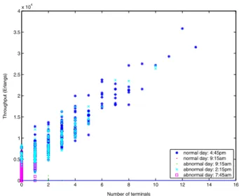
Invariant relation – throughput We examine the
throughput as a function of the number of active user ter-minals in the system. Both the actual measurements col-lected from the UTRAN system and the model as described in equation (1) are used in our analysis. Note that there are alternative models to describe the relations between through-put and the number of active terminals.
A simple anomaly detection rule can be set such that the normal throughput should belong to the range of
[T h(minn) , T h(maxn) ], given the number of active usersnin the
system. Using this detection rule, we can easily find that the abnormal throughput shown as squares in Figure 4. It is ob-served that the system behavior at time 7:45am violates the invariant relation between throughput and the number of
ter-0 2 4 6 8 10 12 14 16 0 0.5 1 1.5 2 2.5 3 3.5 4x 10 4 Number of terminals Throughput (Erlangs) normal day: 4:45pm normal day: 9:15am abnormal day: 9:15am abnormal day: 2:15pm abnormal day: 7:45am
Figure 4. Measured throughput vs. number of terminals
minals. Later we verified that the system has a serious failure at that moment.
3
Temporal correlations
Trend analysis [4] is an approach to predicting the fu-ture movement of target observations. It is based on the idea that what has happened in the past gives us the idea of what will happen in the future. By examining the UTRAN mea-surements, we observed that the UTRAN data display a pat-tern of fairly regular fluctuations, such ascycles. This repre-sents the characteristics of user activity in UTRAN systems. Regular cycles have a constant interval between successive peaks, which is the period of the cycle. As a result, trend analysis can be used to estimate the future traffic pattern and load in cellular systems.
Different models can be used to model historical behav-iors and changes. One of such models is the regression model. By using regression methods, the trend analysis model takes into account the fact that usage patterns exhibit similarities over time, but they also evolve from time to time. Moving average is one of the methods for detecting trends.
3.1
Trend analysis model
Along time, all UTRAN measurements can be formu-lated as time series. In trend analysis, an observed time se-ries can be decomposed into three components: the trend (long term direction), the seasonal factor (systematic, calen-dar related movements) and the irregular factor (unsystem-atic, short term fluctuations). As a result, a general trend analysis method can be expressed as:
yt=local mean+seasonal factor+error (4)
where the local mean is assumed to have an additive trend term and the error is assumed to have zero mean and con-stant variance. At each time t, the smoothing model es-timates these time-varying components with level, trend,
and seasonal smoothing states denoted byLt,Tt, andSt−i
(i= 0,1, ...M−1), respectively. The set of updating
equa-tions are given by
Lt+1 = α(yt+1−St+1−M) + (1−α)(Lt+Tt)
Tt+1 = β(Lt+1−Lt) + (1−β)Tt
St+1 = γ(yt+1−Lt+1) + (1−γ)St+1−M
whereα,βandγare three convergent matrices of smooth-ing constants, andM is the time interval for a season.
Them-step-ahead forecast at timetis
ˆ
yt+m=Lt+mTt+St+m−M (5)
Note that, the parametersα,β andγof regression mod-els are learned from the past time series by minimizing the errors between the estimated values from models and their actual observations.
3.2
Algorithm
To apply trend analysis in UTRAN time series, we first build a regression model and then perform the prediction with the following steps. Since user activities of UTRAN system reflect daily patterns, a typical trend interval is 24 hours. With different level of observation, other possible trend interval include a week, a month and a year. Here we use “day” as the primary trend interval in our analysis.
1. Determine the seasonal parameterM. 2. Estimate initial values.
3. Estimate parameters ofα,β, andγof the trend model using historical data.
4. Use trend model to predict next (m) step output.
5. Updateα,β, andγto minimize error for the lastktime inter-vals.
6. repeat 4 - 5 with new measures.
Off-line methods can be used for the first three steps to deter-mine or estimate the required parameters. Once the regres-sion model is initiated, on-line algorithms can be used to fit the model with the new measures continuously. Further, time series along with their trend component and seasonal factors can be used as an indicator to detect abnormal system states.
Trend analysis for fault detection Time series along
with their trend component and seasonal factors can be used as an indicator to detect abnormal system states. For exam-ple, the deviation between the observation and the estima-tion can be used to generate warning for fault detecestima-tion. By collectively considering multiple time series from UTRAN measurements, more comprehensive detection methods can be setup to improve the accuracy of fault detection. Using multiple features (e.g. KPIs) of measurements for UTRAN system management will be discussed in Section 4.
3.3
Experimental results
In this section, we present the evaluation results with data collected from real UTRAN system during the period from May 30, 2006 to June 15, 2006. Each time tick represents a 15-minutes interval, and there are 96 time ticks for a day.
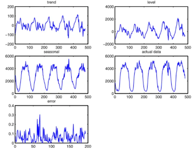
3.3.1 Example 1: Throughput in terms of bear services
In this example, the time series is decomposed into three parts: trend, seasonal factor and levels. Follow the steps list in the previous section, the parameters are learned with historical data. 0 100 200 300 400 500 −200 −100 0 100 200 trend 0 100 200 300 400 500 −2000 0 2000 4000 level 0 100 200 300 400 500 0 2000 4000 6000 seasonal 0 100 200 300 400 500 0 2000 4000 6000 actual data 0 50 100 150 200 0 0.1 0.2 0.3 0.4 error
Figure 5. Throughput with trend analysis: June 9, 2006 to June 15, 2006
As shown in Figure 5, the trend has relatively small fluc-tuation comparing to seasonal factor, which means that the trend is relatively stable for throughput. On the other hand, the seasonal factor has obvious fluctuation within one day. That is, for one day cycle, the system has peak throughput during the daytime, and the system has lowest throughput around 3:00am in the morning every day, shown as “sea-sonal” in the figure. The level of throughput shown as “level” represent the irregular part of the cycle each day. This is the part that reflects the daily change of throughput. The esti-mation error (zoomed to show only the first two days) with actual measurement is normalized and shown in Figure 5. It is noticed that on June 10, there is larger error than the mean errors, and something irregular is detected by our trend anal-ysis. We checked the actual data and found that the system did not respond well for a 30-minutes interval during that midnight.
4
Cell correlation
A mobile cellular system may include hundreds of cells with a large number of KPIs, which reflects the correlated relations between different cells. The challenge of cell cor-relations is how to define the similarities among cells with respect to the KPIs. In this section, we first examine the cell correlation with respect to a single KPI and then we apply a signature vector to examine multiple KPIs for cell correla-tions. We also propose to use parallel and sequential meth-ods to evaluate system states with multiple KPIs.
4.1
Single KPI-based cell correlation
Based on the importance of KPIs, a few selected KPIs can be used to examine cell correlations. As a result, the
feature (e.g. normal behaviors) of each cell can be charac-terized by those selected KPIs. Faulty cells can be located by comparing KPIs of different cells. Since cells can be cor-related based on different KPIs, the correlation results can be different with respect to different KPIs. Since there exist correlations between different KPIs, it is expected that the feature of one KPI could convolve with another KPI.
The steps of using selected KPIs for fault detection is as follows. First, each cell is correlated with other cells based on a given KPI. Secondly, based on certain criteria (e.g., comparing the correlation value with pre-defined threshold), the cells are grouped as normal and suspicious. Further, other KPIs of suspicious cells are cross-checked. If the same cell is also raised as “suspicious” with other KPIs, that cell may require further analysis to determine root causes. Cells can also be correlated with each individual KPI in parallel and cross-checking the correlation results using binary oper-ation such asandoror, which can be expressed as:
F aultyCells = SuspiciousCells(KP I1)∧
SuspiciousCells(KP I2)∧
... SuspiciousCells(KP Ik)
where, the number of selected KPIs isk, and is much less than the total available KPIs, andSuspiciousCells(KP Ii)
is the set of cells which violates the rules set forKP Ii. As
a result,F aultyCellsis the set of cells which violates all rules ofKP Ii(i = 1,2, ...k). With selected KPIs, the sys-tem status can be examined at a finer level. Note that not all suspicious cells are faulty. However, suspicious cells have high possibility to be faulty and can be confirmed either by cross-checking with other KPIs or with additional monitor-ing data.
4.2
Experimental result for single KPI
based cell correlation
0 10 20 30 40 50 60 70 80 90 100 50 100 150 200 Time
Total received power
cell 599 cell 591 cell 590 cell 283 cell 217 cell 657
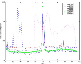
Figure 6. An example of single KPI-based cell correlation
In this experiment, cells are first grouped based on a given KPI (e.g. downlink interference in terms of received power). Most cells present relatively stable interference over time.
However, several cells, such as cell 217, 283, 657, 590, 591, 599 exhibit large fluctuation during a day by violating re-ceived power threshold, as shown in Figure 6. By cross checking with other KPIs such as RRC success rate, cell 599 is malfunctioned during 7:00pm-7:15pm by experienc-ing much lower success rate. After the performance problem from the cell is solved, the system went back to normal be-haviors later in that day. Although other suspicious cells also experience high interference, they have heavier load than normal and do not reveal problems with other KPIs. This method can facilitate operators to narrow down the problem size from hundreds of cells to several cells, and therefore, greatly reduce the complexity in data analysis.
4.3
Multiple KPIs-based cell correlation
In this section, the combination of multiple KPIs for cell correlation is discussed using the concept of signature vector.
4.3.1 Signature vector of KPIs
Now we can use the reduced number of KPIs from Section 2 to formulate a KPI vector to define the state of system or cells. Since the elements of KPI vector have varied range of values, the KPI vector should be normalized before fur-ther processing. Each element in the vector is normalized to the range between[0,1]. Different methods can be applied for this normalization. For example, a rule can be used to distinguish normal and suspicious behavior of a KPI, which result in a binary representation of that KPI. Here we in-troduce a “signature” vector to describe the normalized KPI vector. An example of the signature vector is expressed
as SV = [0,1, ...,0]. In general, multi-level quantization
(based on more complex rules or mathematic properties) can also be used for normalization. By using a signature vector to represent the system state, the noises from original KPI values would be filtered and the system state space would be highly compressed.
After the signature vectors are obtained, for repeated problems, they can be mapped into specific problems based on codebook correlation approach [11]. For example, if sig-nature vector for problem 1 is [1 1 1 0 1], and sigsig-nature vec-tor for problem 2 is [1 1 0 1 1], they are added to the code-book. Next time, when a specific signature, such as [1 1 1 0 1] (if the detection distance is 1) is observed, the root cause can be identified promptly. That is, with the preprocessing of codebook and corresponding causes, fault diagnosis and on-line analysis with large volume of data become very fast. Note that, the codebook may be different for different time period.
4.3.2 Correlation rules
In the transformation of KPI vectors to signature vectors, we use spatial and temporal correlations techniques discussed in previous sections to generate various correlation rules. Dif-ferent correlation methods can be used to derive many rules and then we can merge these rules with the signature vector
0 50 100 0 50 100 150 200 Number of cells State 0 0 50 100 0 50 100 150 200 State 1 0 50 100 0 50 100 150 200 State 2 0 50 100 50 100 150 200 250 time Number of cells State 3 0 50 100 0 50 100 150 200 250 300 350 time State 4 0 50 100 0 1 2 3 4 time State 5
Figure 7. Multi-variate sig-nature vector: normal case
0 50 100 100 200 300 400 500 600 700 800 Number of cells State 0 0 50 100 0 50 100 150 200 250 State 1 0 50 100 0 50 100 150 200 250 300 State 2 0 50 100 0 50 100 150 200 250 300 time Number of cells State 3 0 50 100 0 50 100 150 200 250 300 350 time State 4 0 50 100 0 0.5 1 1.5 2 2.5 3 time State 5
Figure 8. Multi-variate sig-nature vector: faulty case
0 20 0 50 100 0 20 0 50 100 0 20 0 50 100 0 20 0 50 100 0 20 0 50 100 0 20 0 50 100 0 20 0 50 100 0 20 0 50 100 0 20 0 50 100 0 20 0 50 100 0 20 0 50 100 0 20 0 50 100 0 20 0 50 100 0 20 0 50 100 0 20 0 50 100 0 20 0 50 100 0 20 0 50 100 0 20 0 50 100 0 20 0 50 100 0 20 0 50 100 0 20 0 50 100 0 20 0 50 100 0 20 0 50 100 0 20 0 50 100 0 20 0 50 100 0 20 0 50 100 0 20 0 50 100 0 20 0 50 100 0 20 0 50 100 0 20 0 50 100 0 20 0 50 100 0 20 0 50 100 0 20 0 50 100 0 20 0 50 100 0 20 0 100 200 0 20 0 100 200 0 20 0 100 200 0 20 0 100 200 0 20 0 100 200 0 20 0 100 200 0 20 0 100 200 0 20 0 100 200 0 20 0 100 200 0 20 0 100 200 0 20 0 100 200 0 20 0 100 200 0 20 0 100 200 0 20 0 100 200 0 20 0 100 200 0 20 0 100 200 0 20 0 100 200 0 20 0 100 200 0 20 0 100 200 0 20 0 100 200 0 20 0 100 200 0 20 0 100 200 0 20 0 100 200 0 20 0 100 200 0 20 0 100 200 0 20 0 100 200 0 20 0 100 200 0 20 0 100 200 0 20 0 100 200 0 20 0 100 200 0 20 0 100 200 0 20 0 100 200 0 20 0 100 200 0 20 0 100 200 0 20 0 100 200 0 20 0 100 200 0 20 0 100 200 0 20 0 100 200 0 20 0 100 200 0 20 0 100 200 0 20 0 100 200 0 20 0 100 200 0 20 0 100 200 0 20 0 100 200 0 20 0 100 200 0 20 0 100 200 0 20 0 100 200 0 20 0 100 200 0 20 0 100 200 0 20 0 100 200 0 20 0 100 200 0 20 0 100 200 0 20 0 100 200 0 20 0 100 200 0 20 0 100 200 0 20 0 100 200 0 20 0 100 200 0 20 0 100 200 0 20 0 100 200 0 20 0 100 200 0 20 0 100 200 0 20 0 50 100
Figure 9. Distribution of cell states over time
to track the whole system. For example, based on the nor-mal behavior of majority of cells, we might choose a thresh-old of the success rate for RRC setup. A cell is considered as suspicious if its rate is much lower than this threshold. Based on historical data, temporal correlation rules can also be set up, as discussed in Section 3. In practice, more com-plicated rules are needed to handle low number of attempts because it is difficult to detect different problems with insuf-ficient statistics. Note that whether a system and/or a cell is at the healthy state is not determined by a single KPI but comprehensive decision rules based on the signature vector. As discussed earlier, all these temporal and spatial correla-tion rules are maintained in a knowledge base. Operators can formulate complicated queries by dynamically combin-ing these rules from the KB to analyze real-time data. We are developing a rule engine which parses such queries and runs these rules on real-time monitoring to extract actionable information.
4.4
Similarity of cells
If the signature vector of one cell is the same as that of another cell, in this paper we say that these two cells have same system states with regard to the signature vector. Note that the similarity of cells is evaluated with the hamming distance between their signature vectors. A simple method to detect the similarity between two signature vectors is to use exclusive disjunction, i.e., “XOR” operator⊕. For example,
v = svi⊕svj, i = j. Two cells are more similar when thevis smaller. With this definition of similarity, we cluster the cells based on the correlation of signature vectors. Many clustering methods [10] for multi-variate parameters can be used for cell grouping purpose such as,k-means and self-organizing maps. It is possible that some of the KPIs are more important than others for system characterization. In this case, we can use weighted KPIs to compare similarity of cells.
To understand the mass behaviors of cells, cells are clus-tered by tracking their signature vectors. With new observa-tions at each time step, we compare those cells in the same cluster to determine any suspicious cell that behaves differ-ently with its peers. In fact, here we use a group of cells with similar behaviors to formulate some common baselines and each cell uses other cells in the same cluster as references
to check its own behavior. This is important because system states keep changing and it’s difficult to verify whether a spe-cific system state is healthy. By comparing with peers, each cell is able to verify whether its dynamic behavior is normal. Such a mechanism is also integrated with our rule engine so that operators can submit a query to fetch such information from real measurements. In addition, such a mechanism can be combined with other correlation mechanisms as a com-plicated query to the rule engine and the engine will parse the query and follow its commands to process low-level real data.
4.5
Experimental results for signature
vec-tors
4.5.1 Example 1
In this experiment, we examine the system state by trans-forming a multi-variate (e.g. six-element) signature vector to a single variable. The normal case is shown in Figure 7, where the distribution of cells that belongs to each state has smooth change with respect to time. When the system is disturbed as shown in Figure 8, it is observed that there is a sudden change of number of cells in those states (state 0, 1, 2, 3, 4). The corresponding signature vector is [1 1 1 1 1 0], which can be found in the codebook and indicates an issue of performance around 8:00am in the morning. It can also be read from the figures that most cells are in the state 0, 1, and 2 when the load is low and most cells are in the state 3 and 4 when the load is high.
4.5.2 Example 2
In this example, five KPIs related to the success rates for call setup and mobility are used. The normalization rules, such as, if KP Ii > 0.9, then svi = 1, otherwise
svi = 0, are applied to each KPIs in the signature vector.
Cells are clustered based on the signature vectors. The dis-tributions of cells for each 15-minutes interval are plotted in Figure 9, for example, the first box is the cell clustering result during during 23:15pm - 23:30pm. For each conse-quent 15 minutes, an updated distribution of system state is plotted. It is observed that most cells belong to the state 30 during 7:00am-11:00pm, while more cells belongs to state 1
during 11:00pm-7:00am. Such statistical results can be di-rectly used for system state monitoring.
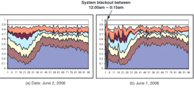
Furthermore, we observe that most cells belong to a small set of all possible system states, such as six states accounting for about 85% of all cells over time as shown in Figure 10. Therefore, we will focus on the dominant states and their associated cells for further analysis. In Figure 10 (b), it is very interesting to observe that at time 12:00am (shown at time tick 3 in the Figure), the whole system has a black-out problem and the expected correlation pattern is violated system-wide. The system states also have physical mean-ings. For example, state 0 means that either success rate of each element is below its threshold, or the number of its at-tempts is close to zero due to very light user load. The state 30 means that most elements in the signature vector has nor-mal success rate. For large dimension signature vectors, we can group the cells based on major system states and they can well reflect the major characteristics of system states.
0 0.1 0.2 0.3 0.4 0.5 0.6 0.7 0.8 0.9 1 16 11 16 21 26 31 36 41 46 51 56 61 66 71 76 81 86 91 96 (b) June 1, 2006 0 0.1 0.2 0.3 0.4 0.5 0.6 0.7 0.8 0.9 1 16 11 16 21 26 31 36 41 46 51 56 61 66 71 76 81 86 91 96
(a) Date: June 2, 2006
System blackout between 12:00am -- 0:15am
Figure 10. Using six states to examine the sta-tus of cellular system
5
Related work
Advanced monitoring and management of large number of performance measurements is an emerging research topic for UTRAN systems [7, 1, 8, 9, 2]. For UMTS performance measurements, we need to implement sophisticated filter-ing/call trace analysis processes in performance measure-ment (PM) software [6]. In [7], the self-organizing mapping andk-means methods are used for clustering and analyzing 3G cellular networks. These algorithms are used to visualize and group similarly behaving cells. However, such methods does not provide explicit physical meaning for the cell be-haviors and does not support on-line analysis. Our method is orthogonal to their method by using spatial and temporal correlations for real time analysis.
In [1], competitive neural method is used for fault detec-tion and diagnosis for cellular system. A given neural model is trained with data vectors representing normal behavior of a CDMA2000 cellular system. We utilize correlation based rules to form signature vector and verify our results with real measurements from cellular system. Another difference is that we use semi-supervised approach when the parameters of the model is required to adapt to the change of the system. Trend analysis has been widely used to track corporate busi-ness metrics [4]. We apply trend analysis to UTRAN system by properly tracking the seasonal factors of KPIs. Temporal
and spatial distributed event correlation are used for network security in [5]. We use spatial and temporal correlations to examine the relations between cells and KPIs in high dimen-sional monitoring data from UTRAN system.
6
Conclusions
In this paper, we present a systematic approach to corre-late performance measurements for mobile cellular network management. We first catalog a large number of raw mea-surements with a limited number of KPIs. Then we exploit the spatial and temporal correlation of KPIs to track and in-terpret system state along time. Experimental results from real UTRAN system demonstrate that it is promising to build a mobile network management and support system by effec-tively correlating KPIs.
References
[1] G. A. Barreto, J. C. C. Mota, L. G. M. Souza, R. A. Frota, and L. Aguayo. Condition monitoring of 3g cellular networks
thorugh competitive neural models. IEEE Transactions on
Neural Networks, 16(5), September 2005.
[2] R. M. S. Gonalves, B. M. G. Miranda, and F. A. B. Cercas.
Mobile network monitoring information system. The 2nd
International Conference on Wireless Broadband and Ultra Wideband Communications (AusWireless 2007), 2007. [3] http://www.3gpp.org/ftp/Specs/html info/32403.htm. 3gpp ts
32.403.
[4] http://www.itl.nist.gov/div898/handbook/pmc. Trend analy-sis.
[5] G. Jiang and G. Cybenko. Temporal and spatial distributed
event correlation for network security. Proceeding of the
2004 American Control Conference, June 2004.
[6] R. Kreher. UMTS Performance Measurement: A Practical
Guide to KPIs for the UTRAN Environment. Willey Publish-ers, 2006.
[7] J. Laiho, K. Raivio, P. Lehtimaki, K. Hatonen, and O. Simula.
Advanced analysis methods for 3g cellular networks. IEEE
Transactions on Wireless Communication, 4(3), May 2005. [8] D. Michel and V. Ramasarma. GPRS KPI measurement
tech-niques for the railway envirionment – lessions learned.Texas Wireless Symposium, 2005.
[9] J. Strassner, B. Menich, and W. Johnson. Providing seamless mobility in wireless networks using autonomic mechanisms.
Lecture Notes in Computer Science, 2007.
[10] R. Xu and D. Wunsch, II. Survey of clustering
algo-rithms. IEEE Transactions on Neural Networks, 16(3):645–
678, May 2005.
[11] S. A. Yemini, S. Kliger, E. Mozes, Y. Yemini, and D. Ohsie.
High speed and robust event correlation.IEEE