Investigations on the application of collaborative visual SLAM using dynamic Ground Control Points

(1)

Leibniz Universit¨at Hannover

Institut f¨ur Photogrammetrie und Geoinformation

Investigations on the application of

collaborative visual SLAM using dynamic

Ground Control Points

Master Thesis

submitted by Yi Huang at 06. Dec. 2019

Professor: Prof. Dr.-Ing. Christian Heipke Supervisor: M.Sc. Philipp Trusheim

(2)

Yi Huang: Investigations on the application of collaborative visual SLAM using dynamic Ground Control Points, Master Thesis, c 06. Dec. 2019

(3)

Erkl¨

arung

Hiermit erkläre ich, dass ich die vorliegende Arbeit selbstständig und ohne fremde Hilfe verfasst und keine anderen Hilfsmittel als angegeben verwendet habe. Die vorliegende Arbeit ist frei von Plagiaten. Alle Ausführungen, die wörtlich oder inhaltlich aus anderen Werken entnommen sind, habe ich als solche kenntlich gemacht. Diese Arbeit wurde in gleicher oder ¨

ahnlicher Form noch bei keinem anderen Prüfer als Prüfungsleistung eingereicht und ist auch noch nicht veröffentlicht.

Hannover, den 06. Dec. 2019

(4)

(5)

Abstract

With the development of autonomous driving, more and more people are studying the tech-nology of simultaneous localization and mapping based on the use of multiple lightweight and cheap camera sensors. Car2X research has also been developed alongside autonomous driv-ing, and information exchange has become an indispensable part. Therefore this thesis will combine information exchange and simultaneous localization and mapping. A vehicle that can transmit its own precise position information is referred to as a dynamic Ground Control Point (GCP), which is expected to assist in the positioning of receiving information vehicles. In order to investigate how to use dynamic GCPs in the collaborative visual simultaneous localization and mapping (CoSLAM), the simulation method is applied.

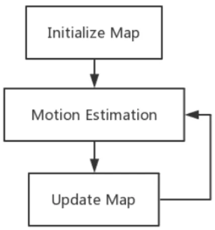
The simulated data include dynamic GCPs, dynamic cameras, and 3D static tie points. The entire implementation process is divided into three steps. The first step is to initialize the map. The exterior orientation of each camera in the first two frames is known, so using the matching 2D feature points and cameras’ exterior orientation in all views of the first two frames to reconstruct 3D static tie points and calculate their covariance matrix. The second step is motion estimation. According to the matching relationship between 3D static tie point and 2D feature point in the new frame, the initial exterior orientation of the camera in the new frame is calculated by EPnP. Then the exterior orientation is optimized by the Levenberg-Marquardt algorithm and the corresponding covariance matrix could be obtained. The third step utilizes the new exterior orientation of each camera to update the old map points and generate new map points. The third and second steps are cycled until the end of the simulation.

Afterward, three scenarios of real road conditions are simulated in the experiment, and the difference between whether to use dynamic GCPs is analyzed. It is found that the camera’s pose error grows slower and even changing its original error trend after using dynamic GCPs when the camera contains motion on both translation and rotation.

(6)

(7)

List of Figures

3.1. Front end and back end in a typical SLAM system [1] . . . 9

3.2. Basic visual SLAM framework . . . 10

3.3. Pinhole camera model [2] . . . 10

3.4. Image (x,y) and camera (xcam,ycam) coordinates [2] . . . 11

3.5. Radial distortion [3] . . . 13

3.6. Schematic diagram for direct method [4] . . . 16

3.7. Feature-based VO . . . 17

3.8. Epipolar geometry constraint [5] . . . 21

3.9. Four possible solutions for relative orientation parameters fromE [2] . . . 24

4.1. Flow chart of main process . . . 36

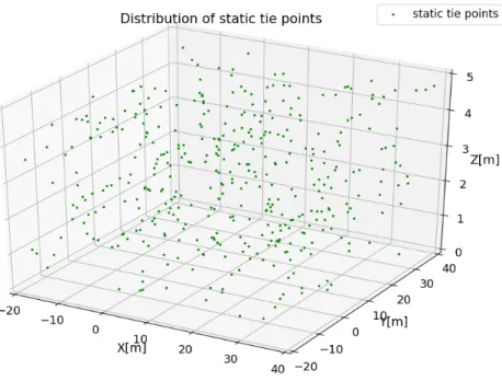
5.1. Distribution of static tie points . . . 44

5.2. Model of scenario A . . . 45

5.3. The number of seen 3D points . . . 46

5.4. The difference between estimated pose and reference . . . 47

5.5. Model of scenario B . . . 49

5.6. The number of seen dynamic GCPs . . . 50

5.7. The difference between estimated pose and reference . . . 51

5.8. Model of scenario C . . . 52

5.9. The number of seen dynamic GCPs . . . 54

(10)

(11)

List of Tables

5.1. The initial positions of camera and dynamic GCPs [m] . . . 45

5.2. RMSE in translation [m] . . . 48

5.3. RMSE in rotation [rad] . . . 48

5.4. The initial positions of cameras and dynamic GCPs [m] . . . 49

5.6. RMSE in rotation [rad] . . . 52

5.7. The initial positions of cameras and dynamic GCPs [m] . . . 53

(12)

(13)

Acronyms

SLAM Simultaneous Localization and Mapping

GNSS Global Navigation Satellite System

CoSLAM Collaborative visual SLAM

GCPs Ground Control Points

SFM Structure from Motion

BA Bundle Adjustment

EKF Extended Kalman Filter

MonoSLAM Monocular Simultaneously Localization and Mapping

PTAM Parallelization of Tracking and Mapping

IMU Inertial Measurement Unit

VO Visual Odometry

DoG Difference-of-Gaussian

SVD Singular Value Decomposition

PnP Perspective-n-Point

DLT Direct Linear Transformation

GN Gauss-Newton

LM Levenberg-Marquardt

BoW Bag of Words

RANSAC Random Sample Consensus

(14)

(15)

1. Introduction

Localization and mapping are essential parts of autonomous driving. Localization deter-mines exterior orientation (pose), mapping integrates the surrounding environment into a model with the help of exterior orientation and observations. The problem of simultaneous localization and mapping is called SLAM [6]. For localization and mapping, the external sensors commonly used are Global Navigation Satellite System (GNSS), camera and laser scanner. It is well known that the above sensors are noisy and there are restrictions on use. Laser scanners accurately sense the environment, but because they are very expensive and cumbersome, they can not be widely used or mounted on small carriers. GNSS has a high demand for the environment. It is suitable for areas with wide fields of vision and fewer obsta-cles. As a result, it usually can not work well in narrow streets. Due to the great attenuation of satellite signals indoors, which results in reduced accuracy, thus GNSS generally does not work well indoors. However, cameras are more likely to work in an unknown environment and could perceive more information such as colors and textures. Hence in recent years, people have gradually explored more possibilities for lighter, smaller, and cheaper cameras [7]. This thesis also aims to investigate the application of the camera. The camera is used as the only external sensor for simultaneous localization and mapping, known as visual SLAM. With the development of Car2X research in the past years, more and more information ex-change will occur. According to the distribution of data information processing space, it can be divided into the centralized processing method and the distributed processing method [8]. In this thesis, localization is based on distributed processing of information, multiple independent cameras are used to improve the localization by collaboration between these sensors. Mapping is based on centralized processing of information, using all useful informa-tion from cameras to generate a more accurate global map. The multi-camera collaborainforma-tion application in visual SLAM is called collaborative visual SLAM (CoSLAM) [9].

Vehicles with accurate position information are called dynamic Ground Control Points (GCPs). The specific task of the thesis is to investigate how dynamic GCPs with known coordinates in image and object space can be used in a CoSLAM by means of simulations. To investigate this question different scenarios should be generated using a given simulation tool. A scenario consists of multiple cameras observing each other and dynamic GCPs. The simulation tool handles three different objects:

1. Dynamic cameras: These are moving cameras that capture the images. The exterior orientation is unknown.

(16)

1. Introduction

2. Dynamic GCPs: These are moving objects with known positions in a global coordinate system at all times.

3. Static tie points: These points are stable in position, their 3D position is unknown. In the simulation tool, the number of cameras, dynamic GCPs and static tie points and their trajectories vary depending on the needs of the scenario. The simulation tool projects the object information into image space and provides the image coordinates of the seen ob-jects. In addition, it also provides the 3D position of every dynamic GCP at each epoch. The main task of this thesis is that using the above data by the CoSLAM to calculate the position of every static tie point and the exterior orientation of every camera in each epoch. In the end, the effect of dynamic GCP on CoSLAM is evaluated by the correctness and accuracy of the results.

The main problem in the implementation process is how to calculate the camera exterior orientation and the application of dynamic GCPs. Since using only the camera as the exter-nal sensor means that there is no other information to predict its own motion, the localization can merely rely on the observations obtained by itself. From a mathematical point of view, there is no motion equation for the model, only the observation equation. Thus, dynamic GCPs are expected to improve the accuracy of cameras’ exterior orientation and static tie points’ position, i.e. controlling the drift of the error. Nonetheless, the number of dynamic GCPs seen by each camera per frame is different. How many dynamic GCPs should be set in order to maximize the positive impact on the results remains to be discussed. At the same time, the distribution of dynamic GCPs should also be analyzed, because the centralized distribution of dynamic GCPs may lead to poor results.

In order to make the structure of this thesis and the content of each chapter clearer, the overall structure of the thesis is presented as follows:

• In chapter 2 the development of SLAM is described. It mainly introduces the work and important achievements of the predecessors in the field of SLAM and highlights the major breakthroughs made in the field of visual SLAM.

• In chapter 3 the theoretical background for visual SLAM is presented. The basic knowledge required to apply the visual SLAM method is explained in detail (such as the theory and formula of photogrammetry and computer vision) and some of the knowledge needed in CoSLAM is also supplemented.

• Inchapter 4 the specific operations and implementation steps to achieve localization and mapping are explained. Principally expounding the implementation method and the setting of the parameters, as well as the application of simulated data.

(17)

• In chapter 5the form and content of the scenario and the setting of the parameters are described. The results of different scenarios about the application of dynamic GCPs are discussed and the correctness and accuracy of the results are also analyzed. • In chapter 6 the conclusion with the application of dynamic GCPs in CoSLAM is in

(18)

(19)

2. Related Work

SLAM allows a robot to perceive the unknown environment, build an environmental map and continuously determine its position according to the environmental map. In 1986 R.C. Smith and P. Cheeseman first propose the probabilistic SLAM problem [10], which is con-sidered the key to achieving a truly autonomous mobile robot. Then in the early 1990s the research group of Hugh F. Durrant-Whyte discusses and solves an open problem (which can be seen as ”which came first, the chicken or the egg?”): localization and mapping depend on each other, accurate localization depends on the correct map, and correct mapping needs accurate location [11]. This discovery stimulates the subsequent research on the SLAM al-gorithm in terms of computational complexity and approximate solution. In 1998 Kalman filter-based SLAM is combined with probabilistic localization and mapping by Thrun [12]. After that, the filter-based SLAM algorithm is widely used and becomes the mainstream of the SLAM algorithm [7]. After 2000, SLAM gradually replaces the laser scanner with various cameras as a new research direction, as computer processing performance has been improved significantly. Because of this, SLAM researchers get ideas from the Structure from Motion (SFM) problem [13] and start to introduce the optimization method bundle adjustment (BA) [14] into SLAM. The difference between the optimization method and the filtering method is that the optimization method is not an iterative process, but considers the information in all past frames, i.e. a difference between least squares and maximum likelihood. The first and second sections focus on the important methods of filter-based SLAM and SFM-based SLAM in visual SLAM.

In the past decades, most visual SLAM techniques have been in view of the assumption that the surrounding environment is static. In fact, the surrounding environment exists a lot of moving objects. When these visual SLAM techniques are applied to actual scenes, various problems or even failures occur. Therefore, in recent years, how to apply SLAM in a dynamic environment has become a direction of SLAM research. The third section mainly introduces the SLAM in a dynamic environment closely related to this thesis.

2.1. Filter-based SLAM

In 1990 Smith et al. firstly present the stochastic map which is the representation of un-certain spatial relationships between objects and use the Extended Kalman Filter (EKF) to find an exactness solution [15]. They use EKF to estimate the position of feature (landmark)

(20)

2. Related Work

and of the robot in the state space at the same time. Yet the disadvantage is obvious, the problem of high computational complexity always exist.

Monocular Simultaneously Localization and Mapping (MonoSLAM) is the first real-time monocular visual SLAM system [16]. MonoSLAM uses EKF as the filtering, tracks the sparse feature points, and updates their mean and covariance with state vector that contains the camera’s current state and all landmarks. In EKF, the position of each feature point is subject to a Gaussian distribution and an ellipsoid can be used to represent its mean and uncertainty. One of the disadvantages of this algorithm is that sparse points are easily lost. The main disadvantage is that, no matter how the filter equation is sorted and calculated, its computational complexity is at least proportional to the square of the number of landmarks. The reason is that landmarks’ locations are added to the estimated state vector, this is also the reason for difficulty meeting the requirements of constructing large-scale maps and real-time.

In order to be able to apply visual SLAM in a large number of landmarks, Montemerlo et al. [17] propose a new algorithm for updating particle filter which is called FastSLAM. It divides the joint SLAM state into the motion part and the conditional map part. For the purpose of reducing the sampling space, the pose of the robot is expressed by particles with different weights and pose state is recursively estimated with the aid of the particle filter method. In particular, the map is represented by an independent Gaussian distribution, the recursive estimation of the map state uses the EKF method. The advantage of the algorithm is that on the one hand the computational complexity is reduced. On the other hand, the particle filter method directly approximates the model, does not require the control vector and the observation to satisfy the Gaussian distribution. However, the disadvantage is how to deter-mine the number of particles. A large number of particles means they require a large amount of memory and calculation time, but a small number of particles lead to inaccurate results [7].

2.2. SFM-based SLAM

Nistr et al. [18] publish the visual odometry (VO) to gradually solve SFM-based SLAM. For the first time, a system for ego-motion estimation in real-time of a single camera or stereo rig is introduced in detail, including feature extraction, feature matching, and robust estimation. In the following study, the front end mainly refers to the VO.

Klein and Murray [19] propose and implement the parallelization of tracking and map-ping (PTAM), distinguish the front and back ends for the first time (the tracking needs real-time response image data, the map optimization is placed on the back end). PTAM is based on keyframes and two parallel processing threads. The keyframe means, instead

(21)

2.3. SLAM in a dynamic environment

of finely processing each image, several key images are stringed together to optimize their trajectory and map. Two parallel processing threads are tracking and mapping. Specifically, the tracking thread does not modify the map but uses known maps for fast tracking; while the mapping thread focuses on the creation, maintenance, and updating of the map. Even if the mapping thread takes a long time, the tracking thread still has a map to track (if the device is still within the scope of the built map). In addition, PTAM also implements the strategy of relocation. If the number of successful inliers is insufficient (such as image blur-ring, fast motion, etc.), the tracking fails. Then the relocation is started, the current frame already compares the thumbnails of keyframes and selects the most similar keyframe as the prediction of the current frame orientation. The disadvantage of PTAM is that the scene is small and the tracking is easy to lose when the camera moves fast or tracks moving objects. In 2015 Mur-Artal et al. propose the monocular ORB-SLAM [20] and in 2016 expand SLAM to get SLAM2 which supports for stereo and RGBD sensors [21]. ORB-SLAM innovatively uses three threads to complete ORB-SLAM, which adds a separate loop closing thread to the PTAM algorithm framework. In addition, the PTAM algorithm framework has been improved: 1) ORB-SLAM tracking, mapping, relocation and loop closing all use uniform ORB features [22], ORB feature’s calculation efficiency is better than SIFT [23] or SURF [24] and has good rotation and scaling invariance; 2) thanks to the use of the visibility graph, the tracking and mapping operations are concentrated in a local cross-view area, enabling them to operate in real-time on a wide range of scenes without depending on the size of the overall map; 3) uses a unified Bag-of-Words model to perform relocation, loop closing and indexing to improve detection speed; 4) improves the lack of PTAM (can only manually select the initialization from planar scenes) and proposes a new automatic robust system initialization strategy on the basis of model selection, allows reliable automatic initialization from planar or non-planar scenes. Yet the downside is that on the one hand, it takes a lot of time to calculate the ORB feature for each image and the three-threads architecture puts a heavy burden on the CPU. On the other hand, a sparse feature point map can only meet the po-sitioning requirements, but can not provide navigation, obstacle avoidance or other functions.

2.3. SLAM in a dynamic environment

To deal with SLAM in a dynamic environment, mainly distinguishing between static and dynamic objects. That is motion segmentation which classifies dynamic and static features, which relies chiefly on computational geometric models (e.g., fundamental matrix, homogra-phy) and sometimes requires the help of an inertial measurement unit (IMU). There are five technologies to segment static and dynamic features: background-foreground initialization, geometric constraint, optical flow, ego-motion constraint, and deep learning [25]. The simu-lation in this thesis already contains distinguished static and dynamic points. Since the idea

(22)

2. Related Work

of the thesis is based on CoSLAM in Zou and Tan’s paper, the motion segmentation of Zou and Tan’s paper applies the reprojection error method of geometric constraint technology, thus only geometric constraint is introduced.

Zou and Tan [9] first present CoSLAM which uses multiple cameras to handle pose esti-mation and distinction between static and dynamic features. In terms of pose estiesti-mation, for the dynamic scene they design a multi-camera collaborative optimization scheme and add the dynamic point constraint to the optimization function (minimization of reprojection error). As for the distinction between static points and dynamic points, firstly all points are treated as static points and then are discriminated according to the reprojection error: if the reprojection error of a point for a single camera frame exceeds the threshold, the category of the point is marked as ”unknown”, then combined with the information of other cameras, it can be judged whether the point is a dynamic point. But the biggest limitation when using this method in the real world is to require time synchronization for each camera.

Tan et al. [26] use a similar approach with Zou and Tan [9], but they consider occlusion to make the results more robust. Projecting feature points to the current frame can compare appearance and structure, then it could be found that if this area has changed, i.e. whether the area may be occluded due to the change of perspective. The invalid 3D points can be deleted and updated in a timely and efficient manner so that the system can cope well with gradually changing scenes. The problem remains that fast moving objects can lead to failure, and the system can only work in a small range.

(23)

3. Theoretical Background

In 2016 Cadena et al. [1] talk about the past, present and future of SLAM. They not only evaluate and affirm the past work, but also propose the direction for the development of SLAM, as well as a typical system of SLAM is given in In Fig. 3.1. This system consists mainly of two parts: the front end and the back end. The front end performs data processing and integration, the back end performs inference estimation, the important loop closing step requires feedback from the back end and data from the front end to promote a more robust system.

Figure 3.1.:Front end and back end in a typical SLAM system [1]

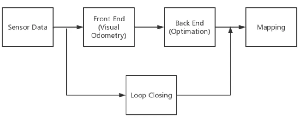
On the basis of the SLAM structure in the above Fig. 3.1, the basic visual SLAM frame-work is summarized in Fig. 3.2. The basic visual SLAM frameframe-work includes 5 components: sensor data, front end, back end, mapping and loop closing. Since this thesis is based on monocular cameras, the detailed description of these important components is only relevant to monocular cameras. Section 3.1 explains the staple model of the camera, including imaging principle, coordinate transformation, and distortion. The section 3.2 introduces the reading and preprocessing of camera data. The front end is presented in section 3.3 and is also known as VO. It expounds on how to quantitatively estimate the motion of the camera from images of adjacent frames. Section 3.4 describes the back end which optimizes the results of the front end. Loop closing in the section 3.5 usually determines whether the camera appears in the previous position by judging the similarity of the image, thus solving the problem of position drift over time. Mapping is based on different sensor types and application requirements. Section 3.6 briefly introduces the common maps.

(24)

3. Theoretical Background

Figure 3.2.: Basic visual SLAM framework

3.1. Camera model

The process of a monocular camera mapping points in the world coordinate system to the image pixel coordinate system can be expressed by a simple pinhole model. However, by reason of the presence of the camera lens, the above process is distorted. Wherefore the next two sections focus on a pinhole model and distortion.

3.1.1. Pinhole camera model

Figure 3.3.: Pinhole camera model [2]

The pinhole camera model in Fig. 3.3 shows the central projection of a point with global coordinate X = [X,Y,Z]T onto the image planeZ = f. The line connecting point X and

(25)

3.1. Camera model

camera center C intersects the image plane at point x. Assuming that the principle point

p is the origin of coordinate in the image plane, according to the similarity of triangles the coordinate of pointx is [fX_Z,fY_Z,f]T. Ignoring the last item, the 2D camera coordinates of point xis [fX_Z,fY_Z]T. Yet actually it exists principal point offset shown in Fig. 3.4, the true image coordinates of point xis [fX_Z +px,fY_Z +py]T [2].

Figure 3.4.: Image (x,y) and camera (xcam,ycam) coordinates [2]

If pointXand point xare represented in homogeneous coordinates, the central projection is able to be simply signified as a linear mapping between their homogeneous coordinates, which is expressed as a matrix multiplication:



   

f X +Zpx

f Y +Zpy

Z      =     

f 0 px 0

0 f py 0

0 0 1 0

             X Y Z 1         (3.1) K=     

f 0 px

0 f py

0 0 1

     (3.2)

The matrix K is called calibration matrix, the 3 parameters of calibration matrix K are called interior orientation. The above formula is derived based on assumptions that camera center C is the origin of the global coordinate, it means that the point X is in the camera coordinate system, so [X,Y,Z, 1]T can be written as Xcam. Then the Equ. 3.1 can be

(26)

x=K[I |0]Xcam (3.3)

However generally, the camera center Cis not the origin of the global coordinate system. Therefore pointXshould be convert from global coordinate system to the camera coordinate system through the transformation matrix Tcam_global first. The transformation matrix Tglobal_cam

include 3×3 rotation matrixRthat represents orientation of camera coordinate system and 3×1 translation vectortthat represents camera center position in global coordinate system. Rotation matrix Rand translation vector t together are called exterior orientation.

T_camglobal=





R t

0T 1



 (3.4)

T_globalcam =T_camglobal−1 =





RT −RTt

0T 1



 (3.5)

The mapping of pointXfrom global coordinate to camera coordinate is shown in Equ. 3.6:

Xcam =





RT −RTt

0T 1

          X Y Z 1         =  

RT −RTt

0T 1



X (3.6)

Combining Equ. 3.3 with the above formula 3.6 to get the following formula:

x∼K RT [I | −t]X (3.7)

The projection matrix Pis determined by the calibration matrix and the transformation matrix:

P =K RT [I | −t] (3.8)

3.1.2. Distortion

The lens in front of the camera affects the propagation of light during imaging. For ex-ample, irregular refraction of light is produced as it passes through the lens. The closer to the edge of the image, the more obvious the tendency that a straight line through the lens becomes a curve on the image. This phenomenon is called distortion. Distortion can be generally grouped into radial distortion and tangential distortion [27]. Radial distortion is induced by an imperfect lens manufacturing process that can result in defects in the shape of

(27)

3.2. Sensor data

the lens. Radial distortion [3] mainly includes barrel distortion with positive radial displace-ment and pincushion distortion with negative radial displacedisplace-ment. Normal image without distortion (a), barrel distortion (b) and pincushion distortion (c) are shown in Fig. 3.5:

Figure 3.5.: Radial distortion [3]

A radial distortion model is exhibited in Equ. 3.9 and Equ. 3.10 [28]:

∆xr=xcam(k1(x2cam+ycam2 ) +k2(x2cam+ycam2 )2+k3(x2cam+y2cam)4) (3.9)

∆yr =ycam(k1(x2cam+ycam2 ) +k2(x2cam+ycam2 )2+k3(x2cam+y2cam)4) (3.10)

where xcam and ycam are arbitrary coordinates in the image coordinate system, k1,k2,k3

are parameters of radial distortion.

Due to the fact that the lens is not parallel to the image plane, tangential distortion takes place [29]. In general, radial distortion affects the image a lot than tangential distortion, which means radial distortion is less credible and needs to be corrected [30]. A tangential distortion model is shown in Equ. 3.11 and Equ. 3.12 [28] with p1, p2 as parameters of

tangential distortion:

∆xt= 2p1xcamycam+p2((x2cam+ycam2 )2+ 2x2cam) (3.11)

∆yt=p1((x2cam+y2cam)2+ 2y2cam) + 2p2xcamycam (3.12)

3.2. Sensor data

In visual SLAM the common visual sensors include monocular, stereo and RGB-D cam-eras. A monocular camera has only one camera, a stereo camera has two cameras, and an RGB-D camera usually carries multiple cameras. In addition, RGB-D cameras could capture

(28)

color images. In this thesis, only needed monocular cameras is presented.

The advantages of the monocular camera are the simple structure, low cost, besides that it is easy to calibrate and identify. The disadvantage is that in a single image, the true size of an object cannot be determined. If two images are obtained by the motion of the camera, the distance of the camera motion can be calculated. However, this distance is uncertain and diffs from the real distance by a scale. For this reason that in feature-based monocular slam, the monocular camera is usually initialized by panning. Then the absolute length of the relative translation is fixed to 1, the depth of objects can also be calculated by triangulation. Hence the size of the camera trajectory and the map can be gained in the monocular SLAM, although it still differs from the real trajectory and map by a real scale.

Calibration should be performed first before the experiment begins. The purpose is to establish the relationship between the global coordinate system and the image coordinate system. Therefore, the parameters required to be solved include interior parameters, exte-rior parameters, and distortion parameters. ”Zhang’s Algorithm” is a camera calibration method using a one-sided checkerboard [31]. This method not only conquers the disadvan-tages of high-precision calibration required by the traditional calibration but also supplies higher accuracy and more convenient operation compared to self-calibration. Thus, Zhang’s algorithm is encapsulated as the function and widely used in computer vision. The actual steps for camera calibration refer to the paper [31].

3.3. Front end

VO estimates the relative pose of the camera on the basis of two adjacent frames. Since this estimate is affected by noise, the estimation error of the previous frame is added to the motion of the subsequent frame, this phenomenon is called drift. In other words, the cumulative error of VO over time leads to pose drift. Therefore, VO can only be used as the front end which estimates the rough result that used as the initial value of the back end. According to the difference of used image information the implementation method of VO can be grouped into the direct method using gray information and the feature-based method. The next two sections will focus on the feature-based method and briefly introduce the direct method for the reason that the feature method is steady and insensate to illumination and dynamic objects.

3.3.1. Direct method

The direct method doesn’t depend on feature points because not only it takes a lot of time and computation to extract and match feature points, but also the process of extracting feature points from an image discards a lot of useful information in the image. Thence the

(29)

3.3. Front end

direct method skips the step of extracting the feature points and estimates the motion by minimizing the photometric error instead of minimizing the reprojection error. In addition, because the direct method uses more information about image pixels, it is more robust in the poorly textured part than the feature-based method. The direct method saves the time of feature extraction, but if a large amount of image information is used for motion estimation, the large optimization problem in the later stage requires a large amount of computation to solve, so that the direct method can only achieve real-time through GPU acceleration.

According to the number of used pixels, the direct method is grouped into sparse direct method, dense direct method and semi-dense direct method [32]:

• Sparse Direct Method: Choosing sparse keypoints but not requiring descriptors, so the calculation and matching of descriptors can be avoid to make calculations simpler. The reconstruction depends on sparse keypoints.

• Semi-dense Direct Method: Consider using only pixels with gradients and discarding the pixels whose gradients are not obvious because such pixels have no positive effect in motion estimation. Finally performing semi-dense reconstruction.

• Dense Direct Method: All pixels are used for motion estimation and reconstruction, which has high requirements for computation. Yet the built dense map has many functions, such as path planning and obstacle avoidance.

The direct method is on account of the assumption that the gray value is constant, i.e. assuming that the imaged gray value of a point is constant at various views. However, when the illumination changes, the direct method is easy to fail. The reason is that the constraint of gray value invariance requires the luminosity error between two images to be as small as possible. In Fig. 3.6 shows the relationship of point P between space and image and the relationship between two frames. The corresponding pixel points of the point P in the space on the first frame and the second frame image are P1 and P2, respectively. Beyond that,

the relative pose in the following figure is represented by rotation matrix R and translation vector t, it is able to be expressed by the Lie algebraξ (see in appendices A).

In order to obtain the pose of the camera in the second frame relative to the first frame, an optimization problem is established according to the hypothesis of gray value invariance. As shown in Equ. 3.13, the optimal solution is gained by minimizing the photometric error which is represented by the variable e[4].

e=I1(P1)−I2(P2) (3.13)

The optimization function exhibited in Equ. 3.14 is the L2 norm of the photometric error.

min

ξ J(ξ) =||e||

(30)

Figure 3.6.: Schematic diagram for direct method [4]

There are endless points in reality, if each point is represented asPi, then the whole camera

pose estimation problem becomes the Equ. 3.15:

min

ξ J(ξ) = N

X

i=1

eT_i ei (3.15)

where ei is expressed in Equ. 3.16.

ei =I1(P1,i)−I2(P2,i) (3.16)

The specific solution to the above formulas will not be outlined here.

3.3.2. Feature-based method

The feature-based method considers that some representative points should be picked first which called feature points. Thereafter, the motion of the camera is estimated only for these feature points while reckoning the 3D position of the feature points. However, information about other non-feature points in the image is discarded. For each feature point, in order to explain its difference from other points the ”descriptor” is created. A descriptor is usually a vector containing information about feature points and surrounding areas. If the descriptors of two feature points are similar, they can be considered to be the same point. On the basis of the information of the feature points and the descriptors, the matching points in the two images could be calculated. Once the matched feature points are found, the relative pose is

(31)

3.3. Front end

able to be calculated by the epipolar geometry. After the feature points are reconstructed by relative pose, the reprojection errors of the feature points are minimized to obtain the best solution for the pose.

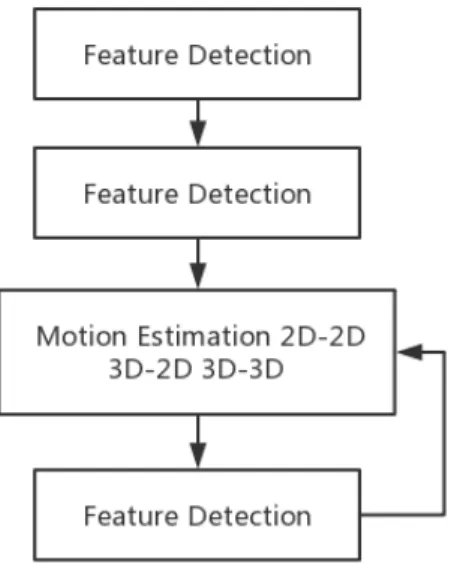
The following flow chart 3.7 shows the entire process of feature-based VO including feature detection, feature matching, motion estimation, and triangulation. They are an indispensable part of VO and have been gradually improved by predecessors [18–20]. Thence, the next few sections will elaborate on the specific implementation steps of the main components of feature-based VO.

Figure 3.7.: Feature-based VO

3.3.2.1. Feature detection

The feature is the representation of image information, high standards are generally re-quired for selected features. For example, they should have invariance to changes of per-spective and illumination and have some flexibility for blur and noise. Relative to the edges and pixel blocks of the image, the corner points with strong local grey value gradients in different directions are easier to calculate and compare their similarities in the two images. For this reason, the corner points become a so-called feature. However, when the observed distance or the perspective changes, the shape or type of the corner point changes so that it cannot be recognized. Thus, scientists in the area of computer vision have studied many more steady local image features, such as SIFT [23], SURF [24], ORB [22], etc. They have different performance in the aspect of rotation, scale invariance, and computational speed.

(32)

The feature consists of two parts: keypoint and descriptor. Examples for keypoint are Harris corners [33], Shi-Tomasi corners [34] and FAST corners [35]. Feature descriptor contains BRIEF [36], BRISK [37], SURF, SIFT, ORB, etc. The next paragraphs will deal with the basic steps of SIFT, SURF and ORB and their respective highlights.

The full name of SIFT is the Scale Invariant Feature Transform which presented in 2004 by Canadian professor David G. Lowe [23]. SIFT feature is a very stable local feature because it is scale and rotation invariant. The SIFT algorithm has the following main steps:

• Create different resolutions of image: That is the construction of Difference-of-Gaussian (DoG) Pyramid. A pyramid with a linear relationship (scale space) is constructed so that the feature points of the image can be found on the continuous Gaussian kernel scale. In addition, using a first-order DoG function to approximate a Gaussian Laplacian is equivalent to approximately calculate the most stable feature of an image, while greatly reducing the amount of computation.

• Keypoint localization: First, keypoint is selected by the local extrema of the DoG scale space, and then the low-contrast points and the unstable edge response points are removed to obtain the true keypoint.

• Orientation assignment: A gradient direction histogram is generated on account of the local image gradient direction, and the peak of the gradient direction histogram yields a dominant keypoint direction. All further orientations are computed relative to this dominant direction.

• Keypoint descriptor construction: Based on position, direction, and scale information of the SIFT keypoint a set of vectors is applied to depict the information of the keypoint and its surrounding neighborhood pixels.

SIFT is based on lots of heuristics and free parameters, and it is extensively used in com-puter vision and photogrammetry. Nonetheless, the shortcoming of SIFT is that there is no global control in local method and no perspective invariance.

On the basis of the SIFT algorithm SURF (Speeded Up Robust Features) [24] mainly improves the defects of the SIFT algorithm, such as slow operation speed and large calculation amount. The SURF process is similar to SIFT, hence only improvements are reflected in the following aspects:

• SURF relies on Hessian matrix to transform images, and the positions of keypoints are detected according to the extremum of the Hessian matrix determinant. Apart from the above step, using box blur filtering to approximate Gaussian blur.

• SURF builds scale pyramids by keeping the image size constant but changing the size of the box filter instead of downsampling.

(33)

3.3. Front end

• SURF uses the response of the first-order Haar wavelet in both x and y directions as the distribution information of the constructed feature vector which improves matching speed.

ORB (Oriented FAST and Rotated BRIEF) [22] is a very good real-time image feature extraction and description algorithm. ORB improves the FAST (Features from Accelerated Segment Test) feature extraction algorithm and uses the extremely fast binary descriptor BRIEF (Binary Robust Independent Elementary Features). FAST detects where the gray value of a local pixel changes significantly. This means if a pixel is obviously different from the surrounding neighborhood, the pixel can be considered a corner point. Within the neighborhood of a keypoint in BRIEF, n pairs of pixels pi,qi (i = 1, 2, ..., n) are selected.

Then comparing the gray value of each pixel pairs, if I(pi) > I(qi), 1 is generated in the

binary string, otherwise 0. All pixel pairs are compared to generate a binary string of length n, this binary string is a feature descriptor in BRIEF. The improvements implemented by ORB based on FAST feature extraction algorithm are explained below:

• In order to avoid the excessively concentrated corner points extracted by FAST, non-maximum suppression is applied.

• Aim to extract corner points with high quality, ORB can specify the number n of extracted corner points and then calculate the Harris response value for the extracted corner points. The response values are sorted from large to small, and the first n corner points are selected as the final extracted feature point set.

• Image pyramids are used and corner points on each layer of pyramids are detected to retain scale invariance.

• Intensity Centroid method is employed to maintain the rotation invariance.

3.3.2.2. Feature matching

Feature matching solves data association problems in SLAM, which is to associate the same image parts seen in multiple perspectives. This is accomplished by comparing the distances between descriptors to determine the similarity.

Different distance metrics can be chosen depending on the descriptor. If the type of de-scriptor is floating point, Euclidean distance [38] can be chosen. For a binary [39] dede-scriptor (such as BRIEF), Hamming distance [40] is more suitable. The Hamming distance between two different binaries refers to the number of different bits of two binary strings.

The simplest and most intuitive method is the Brute-Froce Matcher, which calculates the distance between a feature descriptor and all other feature descriptors, and then sorts the

(34)

resulting distances to match the nearest one keypoint. This method is simple, but there are a large number of error matches, which requires some strategy to filter out the wrong matches. Some methods for optimizing Brute-Froce Matcher are described below.

• Twice the minimum distance: choosing twice the minimum distance found in all matched point pairs as the judging criteria. If Hamming distance between a matched point pair is greater than the value, it is considered to be a wrong match and filtered out; if it is less than the value, it is considered to be a correct match.

• Cross matching: Cross matching carries out a Froce Matcher again after Brute-Froce Matcher. If keypoint A is matched to keypoint B by Brute-Brute-Froce Matcher, and point B is once again matched to keypoint A by Brute-Froce Matcher, it is considered to be a correct match.

• KNN matching: K-nearest neighbor matching means that picking K points which have the most similarity with the feature point. If K is 2, that is called KNN bidirectional matching method. For each feature point, there will be 2 matches. If the distance ratio of the first match and the second match is large enough, then this is considered to be a correct match [41].

3.3.2.3. Motion estimation

Motion estimation can be performed based on matched feature points. There are three types of situations in motion estimation. The first is the relative pose estimation between 2D images, the second is the projection relationship calculation between the 3D point cloud and the 2D image, and the third is the similarity transformation reckoning between 3D point clouds.

2D-2D motion estimation The 2D-2D correspondence is usually used for the initialization of the visual SLAM system because there is only 2D-2D data association at the beginning. First of all, the pose estimation between 2D images is explained. The geometric constraint between any two images can be represented by Fig. 3.8. The center of the left camera isOl,

the center of the right camera isOr, and the line connecting centerOl and centerOris called

the baseline. Assuming that the feature points are correctly matched, so the feature point in the left projective plane is pl and its corresponding feature point in the right projective

plane ispr. Image ray Olpl and Orpr intersects at point P in 3D space. PointOl,Or and P

determines a plane called epipolar plane. The intersections of the baseline and the projective planes are respectively el and er called epipole. The intersection lines of the epipolar plane

(35)

3.3. Front end

Figure 3.8.: Epipolar geometry constraint [5]

Coplanarity of pointOl,Or and P is called epipolar constraint which could be represented

using fundamental matrix Fin Equ. 3.17 [2, 42].

pT_r ·F·pl= 0 (3.17)

Fundamental matrix F is a 3×3 matrix that expresses the correspondence between the feature points of an image pair. The F matrix contains the spatial geometric relationship (exterior orientation) of the two images and the camera calibration parameters (interior ori-entation). Since the rank of the F matrix is two and it can be freely scaled, at least seven pairs of feature points are needed to estimate the Fmatrix.

Essential matrix E is a 3×3 matrix which differs from the fundamental matrix F only by the calibration matrix. Kl and Kr (see in Equ. 3.2) are the calibration matrix of the

left and right cameras respectively. The relationship between the essential matrixE and the fundamental matrix Fcan be indicated by Equ. 3.18.

E =K_rT ·F·Kl (3.18)

The E matrix has nine unknown parameters. Since the rank of E matrix is two, singular value has two constraints and epipolar constraint exists, E consists of five degrees of freedom which means that make use of at least five pairs of feature points to estimate E matrix is allowed. In addition to the fundamental matrix and the essential matrix, there is also a matrix called the homography matrixH.Hmatrix describes the mapping of plane in global coordinate system and image coordinate system, it is not introduced here.

(36)

Solving the relative pose depends onEmatrix andFmatrix. The normalized eight-point-algorithm [43] is the easiest way to calculate the fundamental matrix. Therefore, the basic process of solving the fundamental matrix by the eight-point-algorithm is elaborated in detail below, and then the essential matrix through the relationship between the essential matrix and the fundamental matrix is obtained.

To avoid numerical issues, it is necessary to condition the image coordinates within the feature point sets before estimating the fundamental matrix. Firstly determining the center of gravity (xC,l,yC,l) and (xC,r,yC,r) of the feature points in two images. Secondly calculating

the average distances ¯Simg,l and ¯Simg,r of all feature points from the centres of gravity in

image space. Thirdly obtaining the scalesS2D,l =

√

2/S¯img,landS2D,r=

√

2/S¯img,rfor image

coordinate. SupposingN ≥8 feature point pairs extracted on the left and right images are

xl,i and xr,i withi= 1, 2, 3...N, thence conditioning can be expressed in Equ. 3.19.

x0 =T2D·x, T2D =



   

S2D 0 −S2D ·xC

0 S2D −S2D·yC

0 0 1

     (3.19)

After that the conditioned feature points in image coordinate are x0_l_,_i and x0_r_,_i. For each point pairx0_rT_,_i·F·x0_l_,_i = 0 is satisfied. This constraint is able to expressed via the Kronecker product and the vec-Operator: (x0_l_,_i⊗x_r0_,_i)T ·vec(F) = 0. The expanded description can be seen in the Equ. 3.20.



   

(x0_l_,1⊗x0_r_,1)T ... (x0_l_,_N ⊗x0_r_,_N)T



   

·vec(F) = 0 (3.20)

The above formula 3.20 can also be written as Equ. 3.21.

NA9·9f1=N 01 (3.21)

If there is a certain (non-zero) solution, the rank of the coefficient matrix A is at most eight. As F is a homogeneous matrix, the solution is unique in the absence of a scale factor and can be directly solved by a linear algorithm under the premise that the rank of matrix A is eight. Matrix A’s rank may be greater than eight due to noise in the coordinates of the feature points, thus a least-square solution is required which can be solved by Singular Value Decomposition (SVD) in Equ. 3.22.

(37)

3.3. Front end

The solution of f is the singular vector corresponding to the smallest singular value of the coefficient matrix A, that is, the last column vector of the matrix V. The rank of theFmatrix is two because the fundamental matrix has an important characteristic that is the singularity. For the fundamental matrix, nonsingularity means that the calculated epipolar lines don’t coincide. Therefore, a singular constraint is added to correct the matrix F0 derived from f. First of all, SVD is carried out forF0 in Equ. 3.23:

F0 =hf(1 : 3) f(4 : 6) f(7 : 9)

i

=U ·S0·VT (3.23)

where S0 =diag(σ1,σ2,σ3) . Then smallest singular value is set to 0: S=diag(σ1,σ2, 0).

The corrected Fmatrix is obtained by product of U, the corrected S andVT in Equ. 3.24:

F =U ·S·VT (3.24)

The finalF matrix is recovered from the conditioning:

F =T₂T_D_,_r·F ·T2D,l (3.25)

For the essential matrix, the normalized point pairs are substituted into the eight-point-algorithm of F to get the initial E matrix. Then E matrix is also subjected to SVD. Fi-nally reconstructing E matrix with the singular value constraint through replacing S0 =

diag(σ1,σ2,σ3) by S =diag(1/2(σ1+σ2), 1/2(σ1+σ2), 0).

The next step is to recover the camera’s motion based on the estimated essential matrixE, i.e. calculating the external orientation (R is rotation matrix andt is translation vector) of the camera. This process is derived from SVD: E=U ·S·VT withS =diag(1, 1, 0). There are two solutions fort: t1=v3 andt2=−v3 (v3 refers to the last column of matrix V). And

Rhas also two solutions: R1=V ·W·UT and R1 =V ·WT ·UT withW = 

   

0 −1 0

1 0 0

0 0 1



   

.

Fig. 3.9 shows the combinations of two rotation matrix Rand two translation vector tto get four possible solutions. Only in solution (a) the 3D point in both cameras has a positive depth. Thus, as long as substituting any point into four solutions and calculating the depth of the point in two cameras, the correct solution could be outcropped.

3D-2D motion estimation The characteristics of 3D-2D are commonly used in the oper-ation phase of the visual SLAM system. The previous camera pose and the points in 3D space are known. It is necessary to estimate the correspondence between these 3D points and 2D feature points in the current frame. With this correspondence, the Perspective-n-Point

(38)

Figure 3.9.: Four possible solutions for relative orientation parameters from E[2]

(PnP) method can be used to solve the pose. There are many ways to solve PnP problems, such as P3P [44], Direct Linear Transformation (DLT) [2], EPnP [45] and UPnP [46]. Apart from this, BA is able to resolve the PnP problem. DLT and BA are interpreted next.

First introducing DLT, assuming that a 3D homogeneous point X is projected onto the image plane by the 3×4 projection matrix P with twelve unknown parameters to get the feature point x= [u,v, 1]T which can be represented in Equ. 3.26:

x=λP X, P =



   

pT₁ pT₂ pT₃

     (3.26)

The cross product can be applied to eliminate the unknownλ: x×x= 0 i.e. x×P X = 0. This formula can be described in detail by the following equation:



   

0 −1 v

1 0 −u

−v u 0

         

pT₁X pT₂X pT₃X



   

(39)

3.3. Front end

Expanding the above formula 3.27 to get

upT₃X−pT₁X= 0, vpT₃X−pT₂X= 0, upT₂X−vpT₁X= 0 (3.28) Obviously, the third equation in the above equation can be obtained by the first two equations which means each feature point offers two linear constraints on P. Making an assumption that the number of feature points is N (N ≥ 6), a linear system of equations could be listed:

          

−X₁T 0 u1X1T

0 −X₁T v1X1T

..

. ... ...

−XT

N 0 uNXNT

0 −X_NT vNXNT

                p1 p2 p3     

= 0 (3.29)

The Equ. 3.29 can be written as 2NA12·12P1 = 0. Because of the existence of the error

AP does not equal zero, the||p|| is also fixed to 1 due to homogeneous coordinates, thus the SVD can be utilized to solve the problem. Implementing SVD for A: A =U ·S·VT, P is the rightest column of V.

Local BA wants to minimize the reprojection error between image coordinate of observa-tions and reprojected reconstructed 3D points, i.e. minimizing the sum of squares of a large number of nonlinear functions which can be solved by a nonlinear least-squares algorithm. The common algorithms are Gauss-Newton (GN) algorithm and Levenberg-Marquardt (LM) algorithm [47]. In the following description,xis a state vector containing rotation and trans-lation parameters, h is the increment of x. f(x) is a series of nonlinear equations, i.e. reprojection error equations for 3D points. For small ||h|| the GN algorithm performs a first-order Taylor expansion onf(x) to obtain a Jacobian matrixJ of the derivative off(x) with respect tox, which can be seen in Equ. 3.30 [48].

f(x+h)'l(h) =f(x) +∂f(x)

∂x h=f(x) +J(x)h (3.30)

Then the function F(x) is defined in the following formula, which depicts the sum of squares of f(x+h):

F(x+h)'L(h) = 1 2l(h)

T_l₍_h₎

= 1 2f

T_f ₊_hT_JT_f₊1

2h

T_JT_{J h}

=F(x) +hTJTf+1 2h

T_JT_{J h}

(40)

wheref =f(x) and J =J(x). Then calculating the first derivative of L(h) and making it equals zero: L0(h) =JTf+JTJ h= 0, the GN stephgn which minimizes L(h) can be found

in Equ. 3.32.

JTJ hgn=−JTf (3.32)

However, this algorithm does not converge when JTJ is a singular matrix or in ill condi-tion. If the size of the step is too large, the local approximation may not be accurate. LM algorithm implements some improvements on the basis of Gauss-Newton algorithm. Next, the basic principle and specific steps for LM algorithm are explained.

LM algorithm adds damping parameterµto the Equ. 3.32 and the formula can be expressed in Equ. 3.33.

(JTJ+µI)hlm =g, g=−JTf and µ≥0 (3.33)

If the damping parameter µ is small, JTJ dominates which signifies that the quadratic approximation is good and the LM algorithm is closer to the GN algorithm. Otherwise when

µis large,µI occupies a dominant position andhlm appears in the steepest descent direction,

which means that the nearby quadratic approximation is bad.

The steps of LM algorithm are then shown in Alg. 1. Firstly the initial value of the pa-rameters should be determined. k is the number of iterations and starts from zero, kmax

is the maximum number of iterations and is chosen by user. The factor v is initialized to two. The state vectorx is first assigned by the initial input value and then updated by the calculated increment hlm. Matrix A and matrixg come from the Equ. 3.33. Matrix Qxx is

the covariance matrix of state vectorx, which is the inverse of matrixA. The initial value of the damping parameterµis related to the size of the elements inA, whereτ is also selected by user. In stopping criteria, ε1 andε2 are small and positive numbers, which are chosen by

the user. During the iterative process, the condition for controlling the update is the gain ratio%, where the numerator is the gain of the actual nonlinear model and the denominator is the gain predicted by the linear model. If % is large, it means that the linear result nears to the real model, µ should be reduced to bring the next LM algorithm step closer to the GN algorithm step. If % is small, then the linear approximation is very poor,µis needed to be increased. The purpose is to make the next LM algorithm step approaches the steepest descent direction and reduce the step length. At each iteration, judging the value of % and checking if the exit condition is met. If any exit condition is met, outputting the state vector

x and exiting the LM algorithm.

3D-3D motion estimation The 3D-3D data correspondence is mainly used to estimate and correct the cumulative error of the loop, and to calculate a similar transformation that

(41)

3.3. Front end

Algorithm 1 Levenberg-Marquardt method [48]

k:= 0; v:= 2; x:=x0

A:=J(x)TJ(x); g:=J(x)Tf(x)

f ound:= (||g||∞≤ε1); u:=τ ·max{aii}

while (not f ound)and(k < kmax) do

k:=k+ 1; Qxx :=A−1; Solve (A+µI)hlm=−g

if ||hlm|| ≤ε2(||x||+ε2)then

f ound:=true else

xnew :=x+hlm

%:= (F(x)−F(xnew))/((L(0)−L(hlm))

if % >0then x:=xnew

A:=J(x)TJ(x); g:=J(x)Tf(x)

f ound:= (||g||∞≤ε1)

u:=u·max1₃, 1−(2%−1)3 ; v:= 2

else

u:=u·v; v:= 2·v end if

end if end while

can align the loop. It is mainly used for RGB-D cameras and stereo cameras, so it is not mentioned here.

3.3.2.4. Triangulation

After gaining relative pose between two images or among multiple images, triangulation can be exploited to acquire the coordinates of feature points in 3D space. For example in two views, assuminting thatP1 = [pT1,1,pT1,2,pT1,3]T andP2= [pT2,1,pT2,2,pT2,3]T are projection matrix

for two images, the desired homogeneous coordinates of 3D point is X and its corresponding feature points are x1 = [u1,v1, 1]T and x2 = [u2,v2, 1]T. The principle is similar to the DLT

(see in 3.3.2.3) which uses cross product to eliminate the unknown scale. Therefrom each feature point affords two linear constraints on X and the system of linear equations is shown in Equ. 3.34 [2].

(42)

3. Theoretical Background AX =        

u1pT1,3−pT1,1

v1pT1,3−pT1,2

u2pT2,3−pT2,1

v2pT2,3−pT2,2        

X = 0 (3.34)

However, due to the influence of noise, the above equation is always not equal. Therefore, the problem could be solved by the least-squares method (such as SVD). X is the rightest column of V which is decomposed fromA=U ·S·VT.

3.4. Back end

VO can get the relative pose between two frames. Due to the inevitable error accumula-tion, the absolute pose is drift that means it becomes increasingly inaccurate as time goes on. Therefore, with the help of the back end a reliable solution is able to be built. There are two main methods for back end optimization. One is based on the optimization of filtering theory, because of the simplicity EKF [49] is the mainstream method in the early stage which relies on the Markov assumption. Markov assumption is the state of this frame that is only related to the previous frame of the current frame and has nothing to do with the previous frames (like VO), thus it is difficult to achieve global optimization. The other one is nonlinear optimization, it takes all the data into consideration and puts them together for optimization. Although it will increase the amount of calculation, the result is much better. The state of the system is introduced first, then filter-based optimization and nonlinear optimization are expounded in the next two sections.

In the process of visual SLAM, the system can be described by motion equation and observation equation which are shown in Equ. 3.35:

 



xk =fk−1(xk−1,uk−1) +wk−1

lk=hk(xk) +vk

(3.35)

wheref is the motion equation that infers the current state from the previous state based on the input information andh is the observation equation which gives the observation data generated when the camera sees a 3D point. xpresents all unknowns at each timek= 1, 2, ... including cameras’ exterior orientation and landmarks’ 3D position, u is the input control part,w is the system noise,v is the observation noise andl is the observation.

(43)

3.4. Back end

3.4.1. Filter-based optimization

In a linear Gaussian system, the equations of motion and observation are linear, and the two noise terms obey the Gaussian distribution of zero-mean. The linear system is expressed as follows [50]:

              

xk= Φk−1xk−1+Lk−1uk−1+wk−1 lk₌_Ak_xk₊_vk

wk∼N(0,Qk_ww)

vk_∼_N_(0,_Qk ll)

(3.36)

wherexk orxk−1 is the state vector in the current or previous frame. Qk_ww is a covariance matrix of system noise w. Qk

ll is a covariance matrix of observation noise v. These two

covariances are generally set in advance based on experience. Φk−1 is the transfer matrix that is calculated based on the linear relationship between the previous state xk−1 and the current statexk_. _Lk−1 _{is the control matrix which can be obtained on the basis of the linear}

relationship between control partuk−1and states. Akis the design matrix that is gained from the relationship between observation lk and current state xk. For linear Gaussian systems, Bayesian rules can be used to calculate the posterior probability distribution of x which is the derived process of Kalman filter. Kalman filter is an unbiased optimal estimation of the recursive form of linear systems, the derived results are shown as follows:

                    

Qk_xx_,−= Φk−1Qkxx−,+1 Φk−1

T

+Qk_ww−1

ˆ

x₋k = Φk−1xˆ₊k−1+Lk−1uk−1

Kk =Qk_xx_,−Ak T(AkQkxx,−Ak T +MkQkllMk T)

−1

ˆ

xk₊= ˆxk−+Kk(lk−hk(ˆxk−)) Qk_xx_,+= (I−KkAk)Qk_xx_,−

(3.37)

where ˆxk₋ is the predicted state vector and ˆxk₊ is the corrected state vector in the current frame, Qk_xx_,− and Qkxx,+ are covariance matrices corresponding to ˆxk− and ˆxk+, respectively.

K is the Kalman gain calculated by optimal estimation and used to scale the innovation

lk−hk(ˆxk₋). When the predicted state is obtained by the motion equation (see the first equa-tion of Equ. 3.36), the predicted state can be corrected according to the scaled innovaequa-tion.

However, most systems in the real world are not linear, as well as states and noise are not affected by Gaussian distribution. Therefore, it is necessary to linearize the system and approximate the distribution of states and noises with a Gaussian distribution. For EKF,

(44)

the linearization of the Equ. 3.35 can be performed using Taylor-series with the development point xk−1 = ˆxk₊−1:

xk=fk−1(ˆxk+,uk−1,wk−1, 0) +

∂fk−1

∂x

ˆ

xk₊−1 (x

k−1₋_x_ˆk−1

+ ) +

∂fk−1

∂w

ˆ

xk₊−1 w

k−1 _(3.38)

The nonlinear observation equationsh are linearized analogously tof also on the basis of Taylor-series at the development pointxk_{= ˆ}_xk

−: lk=hk(ˆxk−, 0) +

∂hk ∂x ˆ xk −

(xk−xˆk−) +

∂hk ∂v ˆ xk −

vk (3.39)

In the approximation of the linear system, the noise term and the state term are treated as Gaussian distribution. Thus, as long as their mean and covariance matrices are estimated, the state can be described. After such an approximation, the follow-up work is the same as the Kalman filter. So EKF is a direct extension of Kalman filter. The formula given by EKF is consistent with Kalman filter, and the linearized matrix is used instead of the transfer matrix and the design matrix in the Kalman filter. The calculated result of EKF 1. order for the Gauss-Markov-Model is summarized in following equation:

                    

Qk_xx_,− = Φk−1Qkxx−,+1 Φk−1

T

+Gk−1Qkww−1Gk−1T

ˆ

xk

−=fk−1(ˆxk+,uk−1,wk−1, 0)

Kk=Qk_xx_,−Ak T(AkQkxx,−Ak T +Qkll)

−1

ˆ

xk₊= ˆxk₋+Kk(lk−hk(ˆxk₋, 0))

Qk_xx_,+ = (I−KkAk)Qk_xx_,−

(3.40)

where Φk−1 = ∂f_∂xk−1

ˆ

xk₊−1 ,G

k−1 ₌ ∂fk−1

∂w

ˆ

xk₊−1 ,A

k ₌ ∂hk

∂x ˆ xk −

,Mk= ∂hk

∂v ˆ xk − . EKF has some limitations. For example, it only linearizes using first-order Taylor-series expansion at a fixed point and then directly calculates posterior probability based on the linearization result. However, the first-order Taylor-series expansion depends on the nonlin-earity of the observation and state equations. If these equations have a higher-order term (such as 7 order), the first-order Taylor expansion does not necessarily approximate the whole function. Another drawback is the limited storage space of the EKF. EKF needs to store the mean and variance of the state, at the same time maintain and update them. There are a large amount of landmarks in the visual SLAM. If these landmarks are put into the state, the amount of storage will increase squared with the number of states, so EKF is not suitable for large scenes.

(45)

3.4. Back end

3.4.2. Nonlinear optimization

Local BA is used in VO for nonlinear optimization, but only the camera’s pose and land-marks’ position between two adjacent frames are optimized. For back end optimization, all poses and positions of all landmarks for the entire map need to be Optimized, which means that the amount of data is greatly increased. A huge amount of data can cause a sharp increase in computation which is not suitable for real-time. Until the last decade, people gradually realized the sparsity of BA in the SLAM problem, so that it can be used in real-time scenarios [51]. Sparsity refers to the additional sparsity of the Hessian matrix H when some camera states are not associated with landmarks in BA. The method for solving BA with the help of sparsity will be explained next.

The observation equation is expressed in Equ. 3.41:

h(x) :

 



x0 =xc−f_rr₁₃11(₍X_X−₋_ttx)+_x)+r_r₂₃21₍(Y_Y₋−t_t_y)+y)+_rr₃₃31₍(_ZZ₋−t_tz_z)₎

y0 =yc−f_rr12(X−tx)+r22(Y−ty)+r32(Z−tz)

13(X−tx)+r23(Y−ty)+r33(Z−tz)

(3.41)

where camera’s rotation matrix isR=



   

r11 r12 r13

r21 r22 r23

r31 r32 r33 

   

and camera’s translation vector is

t= [txty tz]T. xc,yc and f are interior orientation. [X Y Z]T is the position of 3D point in

global coordinate system. [x0 y0]T is the image coordinate of the 3D point projected on the image. x= [c1, ...,cm,p1, ...,pn]T stands for camera’s exterior orientationci (include rotation

and translation parameters) and landmark’s 3D positionpj. l is the observations, then the

error of this observation ise=l−h(x). Therefore, the overall cost function can be expressed as [52]: 1 2 m X i=1 n X j=1

||eij||2 =

1 2 m X i=1 n X j=1

||l−h(x)||2 (3.42)

When adding a small increment ∆x to the argumentx, the objective function becomes: 1

2||f(x+ ∆x)||

2 _≈ 1

2 m X i=1 n X j=1

||eij +Jc,ij∆ci+Jp,ij∆pj||2 (3.43)

where Jc,ij represents the partial derivative of the entire cost function 3.42 to the camera

pose in the current state, and Jp,ij represents the partial derivative of the function to the