5247.pdf

(1)

LASSO based Resample Model Averaging for

Genetic Association Studies

Jeremy A. Sabourin

A dissertation submitted to the faculty of the University of North Carolina at Chapel Hill in partial fulfillment of the requirements for the degree of Doctor of Philosophy in the Department of Statistics and Operations Research.

Chapel Hill 2013

Approved by:

Andrew B. Nobel

William Valdar

Yufeng Liu

J.S. Marron

(2)

c

(3)

Abstract

JEREMY A. SABOURIN: LASSO based Resample Model Averaging for Genetic Association Studies.

(Under the direction of Andrew B. Nobel and William Valdar.)

Significance testing one SNP at a time has proven useful for identifying genomic

regions that harbor variants affecting human disease. In theory, simultaneous modeling

of multiple loci should help when considering complex diseases affected by multiple

predictors. However, they are typically applied in an ad hoc fashion: conditioning

on the top SNPs, with limited exploration of the model space and no assessment of

how sensitive model choice was to sampling variability. Formal alternatives exist but

are seldom used. When considering complex traits in humans, the genetic model is

most often assumed to be additive only SNP effects. When non-additive effects such as

dominance or overdominance are present, additive only models can be underpowered.

We first present LLARRMA, a resample model averaging based method using the

LASSO that allows for additive. It estimates for each SNP, the probability that it

would be included in a multiple SNP model in alternative realizations of the data. We

show that under simulations based on real GWAS data, that LLARRMA identifies a

set of candidates that is enriched for causal loci relative to single locus analysis.

We next generalize the resample model averaging framework and present

LLARRMA-dawg, a generalized resample model averaging based method using the group LASSO

that allows for additive and non-additive SNP effects. We show that under simulations

(4)

is enriched for causal loci relative to LLARRMA in the presence of non-additive

ef-fects. We examine how the framework for LLARRMA-dawg can be extended to other

problems where multiple model predictors are required to model the effects of a single

variable.

The final portion of this dissertation describes additional information that one may

explore from resample model averaging. Specifically, we examine how one can identify

response specific variable relationships based on the models selected under resampling.

This give the researcher further information about the predictors than the standard

(5)

Acknowledgments

Much of the work described in this dissertation is collaborative, and I am very grateful

for all of the help I have received. In particular, I would like to thank:

• My advisors Andrew Nobel and William Valdar, for their patience, dedication,

and many insightful comments.

• My committee members Yufeng Liu, Steve Marron and Michael Wu, for their

helpful criticism and suggestions.

• Ethan Lange and Leslie Lange for providing data and patiently explaining

scien-tific questions and concepts.

• Andrey Shabalin, Jeff Roach and many others for their additional helpful

com-ments.

(6)

List of Figures

1.1 Displays the structure of DNA from (Ansari, 2001). . . 2

1.2 Representation of the 23 paired chromosomes of the human male;

modified from (Access Excellence, 2009). . . 3

1.3 Comparison of dominant effects to the additive model. . . 8

1.4 An example of the resulting −log₁₀(p-values) from a single locus

regression in a region of high LD from Strange et al. (2010) . . . 11

1.5 An illustration of a crossover adapted from Morgan et al. (1915). . . 12

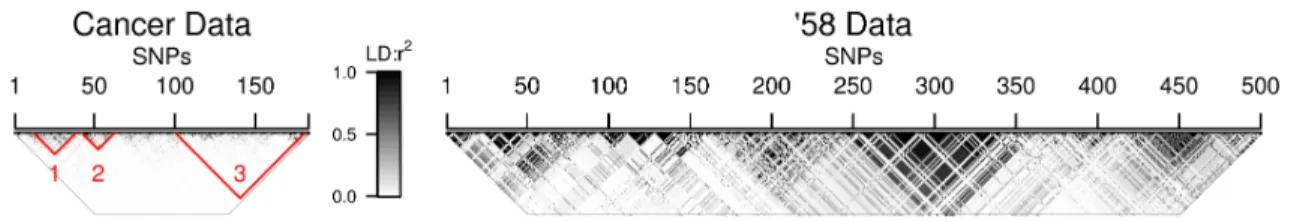
2.1 LD structure of the two genotype datasets used in the simulations. Shading indicates pairwise LD between SNPs, ranging from white

(r2 = 0) to black (r2 = 1). . . 59

2.2 A comparison of LLARRMA and stability selection. . . 64

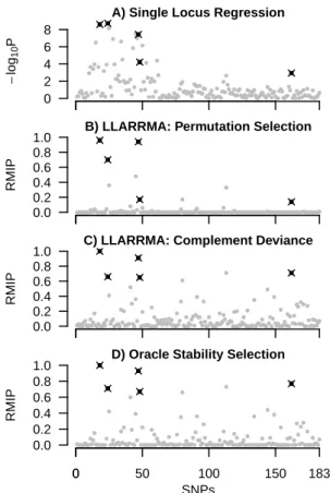
2.3 Results for seven procedures applied to an example case-control data set from simulation study 1A. Plots show SNP score (logP or RMIP) against SNP location in the cancer data, with causal SNPs in black

and non-causal SNPs in gray. . . 67

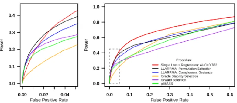
2.4 ROC curves for simulation study 1A: moderate SNP effects in a hit region of moderate LD. Curves compare the ability of seven methods to discriminate causal from non-causal loci in 1000 simulated case-control data sets. Right plot shows the full ROC curve; left plot

shows a zoomed section focusing on the top-scoring SNPs of each method. 68

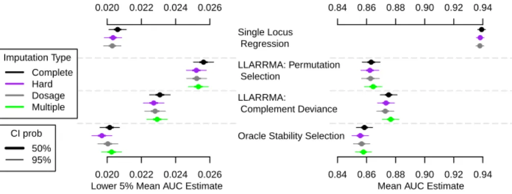
2.5 Area under the ROC curve (AUC) for seven methods applied to four types of imputed genotype data in simulation study 1A: moderate SNP effects in a hit region of moderate LD. Each AUC estimate is based on 1000 simulations and is plotted as mean (dot), 50% CI and

(11)

2.6 ROC curves for simulation study 1B: small SNP effects in a hit region of moderate LD. Curves compare the ability of the methods to discriminate causal from non-causal loci in 1000 simulated case-control data sets. Right plot shows the full ROC curve; left plot

2.7 Area under the ROC curve (AUC) for the methods applied to four types of imputed genotype data in simulation study 1A: moderate SNP effects in a hit region of moderate LD. Each AUC estimate is based on 1000 simulations and is plotted as mean (dot), 50% CI

(thick bar) and 95% CI (thin bar). . . 70

2.8 Global choice of penalty parameter λ by oracle stability selection (black pluses) versus local, per-subsample, choice by LLARRMA complement deviance selection (gray crosses) in 50 representative

simulation trials out of 1000 performed for simulation study 1B. . . 71

2.9 ROC curves for simulation study 2 with 5 loci: small SNP effects in a hit region of strong LD. Curves compare the ability of seven methods to discriminate causal from non-causal loci in 100 simulated case-control data sets. Right plot shows the full ROC curve; left plot

2.10 Area under the ROC curve (AUC) for 7 methods applied to simu-lated case-control influenced by 1-7 causal loci in simulation study 2: small SNP effects in a hit region of strong LD. Each AUC estimate is based on 1000 simulations and is plotted as mean (dot), 50% CI

and 95% CI. . . 72

3.1 LD structure of the HAPGEN2 data sets used in the simulations. Shading indicates pairwise LD between SNPs, ranging from white

(r2 = 0) to black (r2 = 1). . . 90

3.2 Results of four methods applied to an example dataset from sim-ulation study 2B. Plots show SNP score (logP or RMIP) against SNP location in the Hapgen2 data, with true signal SNPs in black (additive effect) and red (non-additive effect) and background SNPs

in gray. . . 94

3.3 Initial and full ROC curves for simulations study 1’s 5 sub-studies. We observe an overwhelming difference between the single locus and multiple locus methods in all situations. We observe consis-tently that LLARRMA-w procedures perform at least as well as

(12)

3.4 Ranking of 2500 true signals from study 1E by single locus regression (SL) vs by LLARRMA-based method (RMA). Colors based on SL significance; genome wide significant (logP ≥ 8; green), marginal

significance (orange), not significant ( logP ≤4; red). . . 98

3.5 The average number of SNPs that must be examined to find the first, second, third, fourth, and fifth true signal in simulation 1E.

Dotted gray line indicates 5% of the SNPs in the hit region. . . 99

3.6 Initial and full ROC curves for simulations study 2A (pa = 0.6, pd=

0.3, and ph = 0.1) and 2B (pa = 0.3, pd = 0.6, ph = 0.1). All

LLARRMA procedures are using their randomized penalties. . . 100

4.1 ROC curves for the additive model based on 100 simulations on HS population A. We observe a clear advantage to methods with either multiple locus modeling (LLARRMA-haplo) or mixed effect models

(EMMA and QTLrel). . . 121

4.2 ROC curves for the full model based on 100 simulations on HS popu-lation A. With the increase to the full model, we observe a advantage

to LLARRMA-haplo over mixed effect models (EMMA and QTLrel). . 122

4.3 ROC curves for the additive model based on 100 simulations on HS population B. We observe a clear advantage to methods with either multiple locus modeling (LLARRMA-haplo) or mixed effect models

(EMMA and QTLrel) with LLARRMA-haplo performing slightly worse. 123

4.4 ROC curves for the full model based on 100 simulations on HS popu-lation A. With the increase to the full model, we observe a advantage

to LLARRMA-haplo over mixed effect models (EMMA and QTLrel). . 123

5.1 Single locus regression and LLARRMA outputs for ARIC African American GWAS data hit region on chromosome 1 for CRP. We observe a large set of significant SNPs in the single locus approach are hard to distinguish between, while the LLARRMA output has

a smaller set of defined SNPs with high RMIPs. . . 131

5.2 Single locus regression and LLARRMA outputs for ARIC African American GWAS data hit region on chromosome 13 for factor 7 levels. We observer both single locus and LLARRMA selecting the same top SNP, but LLARRMA highlights the importance of a

(13)

5.3 LLARRMA and LLARRMA-dawg outputs for ARIC European

Amer-icans hit region for HDL on chr 8. . . 133

5.4 Single locus regression and LLARRMA outputs for MESA European

Americans hit region for CRP on chr 1. . . 134

5.5 LLARRMA-haplo output for HS mice for Mean Adrenal Weight. . . 136

6.1 (Left) displays the LD between SNPs that had RMIPs of at least 0.25. (Right) displays the 2D-RMIP of the same variables. Red lines indicate true SNPs in the model. We observe that the 2D-RMIP does well identifying pairs of variables which have true effects with

the response. . . 139

6.2 RMA based analyses of TCGA breast cancer. (Top) displays the LLARRMA output. (Bottom right) displays ther2 of variables with RMIPs above 0.25. (Bottom left) displays the 2D-RMIP for the

same set of variables. . . 141

6.3 RMA based analyses of TCGA breast cancer luminal subtypes. (Top) displays the LLARRMA output. (Bottom right) displays the

r2 _{of variables with RMIPs above 0.25. (Bottom left) displays the}

(14)

List of Tables

1.1 The base pairs of an individual at 7 loci; we observe that 4 of the 7 loci we have different alleles on each chromatid and the remaining

3 have the same allele. . . 3

1.2 Displays how one models different levels of dominance under the a,

d notation. . . 8

1.3 The base pairs of an individual at 7 loci. The lower half of the table displays the genotypes and phased genotypes of the individual at each loci. The allele sequence of each chromatid are examples of haplotypes. While the genotype row give no indication of the underling haplotypes, in the phased genotypes we notice that the first allele in the phased genotype always corresponds to chromatid 1. This means that the sequence given by the first allele in the

phased genotypes forms the haplotype from chromatid 1. . . 10

3.1 Nomenclature for modeling and resampling procedures used in the

paper. . . 89

3.2 Summary of the sub-simulation models whereβ?_q ∼N(1.35(−1)νj,0.022) withνj ∼Bernoulli(0.5),αis chosen randomly from{0.5,0.75,1,1.25},

and υj ∼Bernoulli(0.5). . . 91

3.3 Mean percent of maximum initial AUC for simulation study 1. All standard errors are less than 0.94. Bold indicates the best method for each model and any methods statistically the same as the best method. Underlined indicates the best method excluding random-ized procedures and any methods statistically the same as the best

non-radomized method. . . 97

3.4 Mean percent of total initial AUC for simulation study 2, where in 2A the true signals effect types are sampled from a Multinomial(5, pa=

0.6, pd= 0.3, ph = 0.1) and 2B from a Multinomial(5, pa = 0.3, pd=

0.6, ph = 0.1) distribution. All standard errors are less than 0.92.

Bold indicates the best method for each model and any methods statistically the same as the best method. Underlined indicates the best method excluding randomized procedures and any methods

(15)

Chapter 1 Introduction

This Dissertation consist of seven chapters. Each chapter addresses a problem or

appli-cation in statistical genetics. Each is related to the general problem of how to identify

genetic variants affecting a given disease trait. This is also commonly known as a

“genetic associations” study.

This chapter provides the necessary genetics background (methods and terminology)

to understand the research problems discussed in the later chapters. The chapter is

laid out as follows. Section 1.1 describes the basic genetics topics that are important

to genetic association studies. Section 1.2 describes the statistical literature on the

human related research problems discussed. Section 1.3 describes the terminology and

literature related to the use of model organisms. Section 1.4 describes how genetic

information is commonly incorporated into a statistical model of association with a

disease trait. Section 1.5 gives an overview of how receiver operator characteristic

(ROC) curves are used to compare methods. The chapter ends with an overview of the

research questions addressed in the dissertation (Section 1.6).

1.1 Basic genetic background

In order to understand fully the statistical modeling of genetic diseases, one needs a

(16)

predictors for a genetic association study, followed by other genetic complications that

often arise within genetic association studies.

1.1.1 DNA structure and SNPs

In the simplest models of association, a single outcome is predicted by a variable

rep-resenting the genetic state of the individual. A common scenario models the state of

individuals differing at a particular variant in their DNA (deoxyribonucleic acid). DNA

carries the genetic instructions used for the development and functioning of all known

living organisms (with the exception of RNA viruses). The information in DNA is

stored as code consisting of four chemical bases: adenine (A), cytosine (C), guanine

(G), and thymine (T). These bases are often referred to as nucleotides, and appear in

pairs. Figure 1.1 displays the structure of the DNA molecule. The pairs come in one of

two forms, A with T or C with G, and form units called base pairs. The DNA molecule

is a long chain of these base pairs separated into long structures called chromosomes.

Figure 1.1: Displays the structure of DNA from (Ansari, 2001).

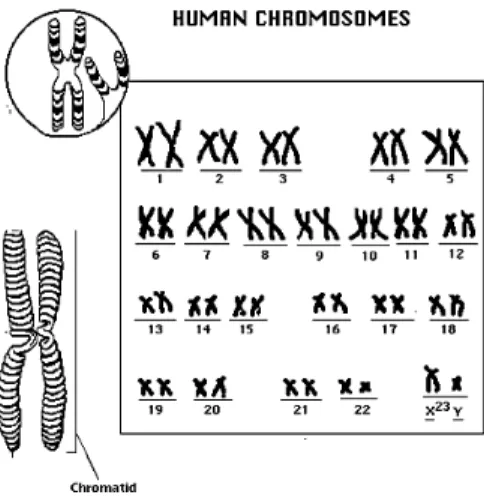
Human DNA comprises of about 3 billion base pairs split over 23 chromosomes, one

of which is our sex chromosome. Figure 1.2 displays the chromosomes of a human male.

More than 99 percent of these bases are the same in all humans. The locations that

differ among individuals are the source of heritable variation in humans (eg. height,

eye color, etc.). Each such location, generically referred to as a locus (plural loci),

potentially harbors variation that affects a trait or disease (often called a phenotype),

and is a candidate predictor for genetic associations. Along with many other organisms,

(17)

Figure 1.2: Representation of the 23 paired chromosomes of the human male; modified from (Access Excellence, 2009).

Locus 1 Locus 2 Locus 3 Locus 4 Locus 5 Locus 6 Locus 7

Chromatid 1 A T C A A G T

Chromatid 2 T T T G A A T

Table 1.1: The base pairs of an individual at 7 loci; we observe that 4 of the 7 loci we have different alleles on each chromatid and the remaining 3 have the same allele.

as homologues chromatids), a paternal copy passed down from our father and a maternal

copy from our mother. As all humans contain two versions of their DNA, each locus

contains two chemical bases (possibly the same). Table 1.1 displays the base pairs of an

individual at 7 loci. Observe that 4 of the 7 loci have different alleles on each chromatid

and the remaining 3 have the same allele. Each chemical base that is observed at a

given location is referred to as an allele. The alleles at a given locus are the predictors

we will consider for genetic association with a phenotype.

The information encoded in one chromatid is called a haplotype. It is often

conve-nient to consider both haplotypes at once. The combination of the two haplotypes at

a single locus is referred to as a genotype. It is most common that a locus where two

individuals’ DNA differs will has only two possible alleles, or nucleotides. Such loci are

(18)

loci that are SNPs. [We will investigate loci that are not SNPs in Chapter 4.] As a SNP

contains only two possible alleles, it is common practice to call the less common allele

in the population the “minor allele”, Q, and the more common allele, q, the “major

allele”.

Given that we know the allele present on each haplotype at a given locus, we can

determine the possible genotypes. The possible genotypes that can be observed are

homozygous minor, QQ, heterozygous, Qq or qQ, and homozygous major, qq. At

present, most techniques for identifying alleles are not capable of resolving haplotypes

of an individual, but merely return the two alleles present at each loci. Thus, it is

common practice to not distinguish between the heterozygous genotypes, Qq and qQ.

With this simplification, the standard additive effect SNP predictor is defined as the

count of the minor allele at a given locus, i.e., we code the unordered genotypes {qq, qQ, QQ} as {0, 1, 2}. With this representation of a SNP, one can begin to see how we may look to statistically model a phenotype as a function of the SNP to detect if

the SNP has a significant additive effect on the phenotype. We consider more general

predictors in Section 1.4.

1.1.2 Genetic models for phenotypic effects

With an understanding of the loci considered for causal variants, one must ask how

these loci affect a phenotype. The underlying genetic models have been disputed, and

exist in many different varieties. The most detailed model would explain phenotypic

variations by including genetic variants, environmental effects, and potential

interac-tions between and within these effects. Models with this level of detail are usually

impractical to estimate and are rarely considered. Simpler models are easier to

under-stand, collect data for, and model statistically. Below describes some of the historically

relevant models that have been used, leading up to the model commonly used in today’s

(19)

Single variant mutations - Mendelian diseases

The origins of genetic association studies come from family based studies of Mendelian

diseases, or diseases resulting from a single mutation in the structure of DNA, which

cause a single basic defect with pathologic consequences. There are thousands of genetic

diseases caused by a single mutation, but discovering which locus is the culprit is still a

daunting task. As Mendelian diseases result from a single mutation, studying the DNA

for multiple generations of a family infected by a disease allows for the identification

of loci that potentially directly results in the disease. While family based studies have

been successful for Mendelian disorders, there remained many diseases for which family

designs were unsuccessful in identifying the underling genetic variants. These diseases

became known as common diseases and their analysis erupted with the introduction of

the genome wide association study (GWAS; WTCCC, 2007).

Simple single locus model - GWAS for common diseases

The simple single locus GWAS model assumes that there is a single SNP variant that

has a causal effect on the phenotype. Unlike the Mendelian model, it is not assumed

that the presence of a single allele determines the disease status of the individual, but

rather it is assumed that the effect of the allele’s count is additive, i.e., the effect of

having two copies of the minor allele is double of that of having a single copy of it. The

effect of locus xi on phenotype y may be modeled as

yi =µ+xi,jβj +i

whereµis the phenotypic mean,βj is the effect of locusxj ony, andi is a normal error.

This simplistic model was one that was assumed in many analyses, and is consistent

with many common diseases. This model is not often considered in today’s literature,

(20)

and potentially interactions of loci and environmental effects. Studies have shown that

phenotypes for complex diseases require multiple variants to explain the differences of

the phenotype (Su, Marchini and Donnelly, 2011). Even though it has become common

practice to assume a more complicated model for complex diseases, it is still common

that studies report only a single locus in their findings.

Simple multiple locus model - complex trait models

As studies have shown that the mendelian model is not valid for complex traits, many

now assume a similar model with contains multiple loci. This model has multiple causal

loci, but for mathematical convenience each locus acts with an independent additive

effect. This may be represented by the the model

yi =µ+

X

j∈J

xi,jβj+i

where J is the set of SNPs with true signals. This model has allowed researchers to account for a much larger amount of variability in complex phenotypes than that

accounted for by the Mendelian model. Even though we assume a multiple locus model,

it is still common practice to test loci one at a time. When considering the simple

multiple locus model, we assume that there exists only a few loci that are truly causal.

This means in statistical terms that we are assuming the model to be sparse.

Genetic dominance in the model

The simple models that we have considered thus far assumed that the SNPs have an

additive effect on the phenotype. Unfortunately, not all genetic effects follow additive

models. By only modeling additive effects, potential causal variants may be missed.

To extend the model further, we remove the assumption of an additive effect to allow

for dominant effects. A dominant effect, in its simplest form, means that having one

(21)

Under this definition, one may also consider recessive effects, meaning having one copy

of the minor allele having the same effect as not having a copy (one may think of a

recessive effect as the major allele is dominant). We will consider a more general notion

of dominance, where by dominance we mean any deviation from an additive model.

The general notion of dominance can be harder to detect, but allows for models

that more closely resembles observed effects. The common genetic dominance model

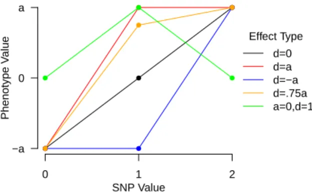
for an individual SNP is to assign two values a and d for the additive and dominant

effect aspects respectively. We assume that the homogeneous minor allele state, QQ,

will have an effect with a value ofa, and the homogeneous major allele state, qq, will

have an effect of −a, and the heterogeneous state, Qq or qQ, will have an effect of d. Under this setting, the coding of the genotypes would differ from the standard 0, 1,

2 coding but be coded as -1, 0, and 1 for qq, qQ, and QQ respectively. This can be

represented in a single locus regression model for locusj as

yi =µ+ajxi,j +djI(xi,j = 0) +i.

Table 1.2 displays how one would write out several models under this notation. This

notation generalizes the additive model to allow a dominant model; it is easily

observ-able that when there is no dominant effect, ie. d= 0, that it simplifies to the standard

additive effects centered at the heterogeneous state. It is also observable that if d=a

(d = −a) that this modeling simplifies to the simplistic definition of a dominant (re-cessive) effect. To illustrate how different dominant effects can be from the standard

additive effects, Figure 1.3 displays the non-additive dominance type effects which the

(22)

Additive Dominant Recessive General Dominance

d 0 a -a a×α ∈_R

qq -a -a -a -a

qQ 0 a -a αa

QQ a a a a

Table 1.2: Displays how one models different levels of dominance under the a, d nota-tion.

0 1 2

−a 0 a

SNP Value

Phenotype V

alue

●

● ●

●

Effect Type

d=0 d=a d=−a d=.75a a=0,d=1

Figure 1.3: Comparison of dominant effects to the additive model.

More general models

As previously mentioned, the most detailed model considered would contain both

ge-netic variants, environmental effects, and interactions between and within these effect.

To account for as detailed of a model containing only genetic effects, one may extend

the multiple locus model to include not only the dominance predictors, but also

inter-actions. Models with interactions are sometimes considered, but are harder to model

statistically; even assuming a sparse model with only considering pairwise interactions,

a very large number of interactions are possible leading to a very large number of

pre-dictors in the model (Balding, 2006). Given the sparse set of causal variants we could fit

a model to include interactions easily, but in this setting it would be more common to

perform a haplotype analysis. A haplotype analysis examines the unique combinations

of each loci, as a haplotype, for association with the phenotype rather than individual

(23)

Locus 1 Locus 2 Locus 3 Locus 4 Locus 5 Locus 6 Locus 7

Chromatid 1 A T C A A G T

Chromatid 2 T T T G A A T

Genotype AT TT CT AG AA AG TT

Phased Genotype A/T T/T C/T A/G A/A G/A T/T

Table 1.3: The base pairs of an individual at 7 loci. The lower half of the table displays the genotypes and phased genotypes of the individual at each loci. The allele sequence of each chromatid are examples of haplotypes. While the genotype row give no indication of the underling haplotypes, in the phased genotypes we notice that the first allele in the phased genotype always corresponds to chromatid 1. This means that the sequence given by the first allele in the phased genotypes forms the haplotype from chromatid 1.

When the contributing loci in a genetic model have been identified, rather than

examine the interactions of the loci, it is more common to phase the data and examine

the individual haplotypes created by the set of loci. By phasing the data, we mean to

analyze the haplotypes in the population and use this information to reconstruct

hap-lotypes from the genotype information. Table 1.3 revisits the data from Table 1.1 and

displays the standard genotype information along with the phased genotypes obtained

after reconstructing the individual haplotypes. As none of the research presented here

is directly related to the use of haplotype phasing, no more details are given here (see

Browning (2008) for further details). With the haplotypes reconstructed, a haplotype

model would assume that each observed haplotype has its own effect. This leads to

a model which can easily be modeled statistically, assuming that you can identify the

proper loci to include in a haplotype. When selecting the loci to include in the

haplo-type model, one needs to consider how fast the size of the model grows, i.e., includingp

SNPs results in 2p possible haplotypes in the model. For this reason, haplotype models

are most often considered for small regions where it is suspected that there are multiple

causal loci, which may not have been validated. This model may include spurious loci

(24)

1.1.3 Linkage disequilibrium

One of the largest hindrances to a genetic association study is the pattern of correlation,

or linkage disequilibrium (LD), between SNPs. LD is considered a measurement of how

likely combinations of alleles would be under the assumption of random formation of

haplotypes. A common measure of LD is the square of the correlation (Balding, 2006).

SNPs that are close together are often in high LD, and this causes a confounding

relationship between the SNPs close to a causal SNP and the phenotype. This often

results in a set of SNPs that form a “cloud” of statistically significant SNPs when

modeled based on single locus methods, as displayed in Figure 1.4. Many standard

statistical methods are unable to distinguish which SNP is the causal SNP within a

set of SNPs in high LD as they fail to incorporate LD information into the analysis

(Balding, 2006).

L E T T E R S

rs27524 at

ERAP1

) generated strong evidence for interaction in the

discovery, replication and combined data (discovery

P

= 2.45 × 10

−5

_,

replication

P

= 0.027, combined

P

= 6.95

× 10

−6

_{) (}

_{Supplementary}

Table 5

).

Figure 3

shows that when stratified by genotypes at the two

loci, the

ERAP1

SNP only has an effect in individuals carrying at least

one copy of the risk allele at rs10484554.

Very few convincing examples of interactions between complex

disease loci have been reported in humans

24–26

_{, perhaps because the}

power to detect these interactions is limited unless the causal SNPs

or very good surrogates have been typed

27

_{. The finding that variation}

at the

ERAP1

locus is only associated with disease in individuals

carrying the

HLA-C

risk allele is particularly interesting biologically

because of the role of

ERAP1

in class I peptide presentation.

It is also noteworthy that the odds ratio for rs27524 is 1.43 (95%

CI 1.21–1.69) in the

HLA-C

–positive subgroup as compared to the

estimate of 1.27 (95% CI 1.18–1.38) from the GWAS of the entire

dataset (in the replication data these estimates were 1.23 (1.09–1.39)

and 1.13 (94% CI 1.05–1.22), respectively). Were this phenomenon

to be more widespread, it would affect the proportion of broad-sense

heritability explained by the GWAS findings.

10 10 8 8 1.0 0 r 2 0.2 0.4 0.6 0.8 6 6 4 4 rs4649203 rs702873 rs17716942 rs6809854 rs280519 rs8016947 rs240993 rs27524 rs458017 rs12720356 rs2278442 rs13014803

LOC284632 REL GCA

GCG

NFKBIA SLC16A10

ERAP1 CAST

KIAA1919 REV3L TRAF3IP2

IFIH1 KCNH7 FAP PEX13C2orf7 KIAA1841 PUS10 IL28RA

1p36 2p16 2q24 3p24

19p13 14q13 6q21 5q15 2 2 0 0 0 0

60.7 61.2 162.6 163.0 163.4 18.6 18.8 19.0 19.2

10.1 35.4 35.2 35.0 34.8 34.6 112.1 111.9 111.7 111.5 96.3 96.2 96.1

96.0 10.3 10.5 10.7

61.1 61.0 60.9 60.8 cM/Mb cM/Mb –log 10 P –log 10 P 10 8 6 4 2 –log 10 P 10 8 6 4 2 –log 10 P 50 50 40 40 30 30 20 20 10 10 0 0 cM/Mb 50 40 30 20 10 0 0 cM/Mb 50 40 30 20 10 10 8 6 4 2 –log 10 P 0 0 cM/Mb 50 40 30 20 10 10 8 6 4 2 –log 10 P 0 0 cM/Mb 50 40 30 20 10 10 10 12 14 8 8 6 6 4 4 2 2 –log 10 P –log 10 P 0 0 0 cM/Mb 50 40 30 20 10 0 cM/Mb 50 40 30 20 10

24.25 24.35 24.45 24.55

Chromosomal position (Mb) Chromosomal position (Mb) Chromosomal position (Mb) Chromosomal position (Mb)

Chromosomal position (Mb) Chromosomal position (Mb)

Figure 2 Regional association plots. The −log₁₀ P values for the SNPs at eight new loci are shown on the upper part of each plot. SNPs are colored based on their r2_{with the labeled hit SNP which has the smallest}_P_{value in the region.}_r2_{is calculated from the 58C control data. Where more than one}

SNP is labeled, there is evidence for multiple signals at the locus (see main text). The bottom section of each plot shows the fine scale recombination rates estimated from individuals in the HapMap population, and genes are marked by horizontal blue lines. Genes within the recombination region of the hit SNPs are labeled, except for 19p13, where the genes are GLP-1, FDX1L, RAVER1, ICAM3, TKY2, CDC37, PDE4A, KEAP1 and S1PR5.

Table 2 Newly associated loci identified in this study

Chr. rsID Positiona _{Gene of interest}b _alleleRisk

RAFc _{Discovery sample} _{Replication sample} _Combined

Cases Controls P_scan OR (95% CI) P_repl OR (95% CI) P_comb

1p36 rs4649203 24,392,507 IL28RA (2) A 0.77 0.73 6.46 × 10−6 _{1.22 (1.12–1.32)} _{1.36 × 10}−3 _{1.13 (1.05–1.22) 6.89 × 10}−8

2p16 rs702873 60,935,046 REL (5) G 0.62 0.56 1.32 × 10−7 _{1.23 (1.14–1.32)} _{1.41 × 10}−3 _{1.12 (1.04–1.20) 3.59 × 10}−9

2q24 rs17716942 162,968,937 IFIH1 (5) A 0.90 0.86 4.05 × 10−8 _{1.38 (1.23–1.54)} _{3.82 × 10}−7 _{1.29 (1.17–1.43) 1.06 × 10}−13

3p24 rs6809854d _18,759,427 _None _G _0.23 _0.19 _{3.09 × 10}−6 _{1.24 (1.14–1.36)} _{4.92 × 10}−3 _{1.14 (1.04–1.26) 1.12 × 10}−7

5q15 rs27524 96,127,700 ERAP1 (2) A 0.40 0.36 6.81 × 10−10_{1.27 (1.18–1.38)} _{7.96 × 10}−4 _{1.13 (1.05–1.22) 2.56 × 10}−11

6q21 rs240993e _111,780,407 _TRAF3IP2₍₄₎ _A _0.30 _0.25 _{8.71 × 10}−13_{1.36 (1.25–1.48)} _{3.37 × 10}−9 _{1.25 (1.16–1.34) 5.29 × 10}−20

rs458017e,f _111,802,784 _G _0.09 _0.06 _{8.11 × 10}−11_{1.62 (1.40–1.88)} _{9.59 × 10}−8 _{1.37 (1.22–1.54) 2.16 × 10}−16

14q13 rs8016947 34,902,417 NFKBIA (1) C 0.61 0.57 4.26 × 10−6 _{1.19 (1.11–1.29)} _{7.89 × 10}−7 _{1.19 (1.11–1.27) 1.52 × 10}−11

19p13 rs12720356g _10,330,975 _TYK2₍₉₎ _A _0.93 _0.90 _{9.25 × 10}−6 _{1.34 (1.18–1.52)} _{8.82 × 10}−7 _{1.40 (1.23–1.61) 4.04 × 10}−11

rs280519g _10,333,933 _A _0.51 _0.47 _{8.51 × 10}−7 _{1.20 (1.12–1.30)} _{5.93 × 10}−4 _{1.13 (1.05–1.21) 4.42 × 10}−9

Evidence for association at loci reported in this study. Chr., chromosome; P_scan, scan stage P; P_repl, replication stage P; P_comb, combined P.

a_{NCBI human genome build 36 coordinates.}b_{The number in brackets shows the number of genes between recombination hotspots.}c_{Risk allele frequency.}d_{This SNP failed Sequenom}

geno-typing, so replication genotyping for this locus was at rs7428395, which had r2_{= 0.97 as calculated from 58C (HapMap CEU}_r2_{= 1).}e_{Separate signals within the same locus, where the}

marginal P values and ORs are reported. For further discussion and details of joint models, see text. f_{This SNP failed Sequenom genotyping, so replication genotyping for this locus was at}

rs465969, which had r2_{= 0.73 as calculated from 58C (HapMap CEU}_r2_{= 0.82).}g_{Separate signals within the same locus, where the marginal}_P_{values and OR are reported.}

© 20

10 Nat

ur

e

Amer

ica,

Inc.

All r

ights r

eser

ved.

Figure 1.4: An example of the resulting−log₁₀(p-values) from a single locus regression in a region of high LD from Strange et al. (2010)

(25)

However LD can also aid genetic analyses, particularly for the imputation of missing

genetic data. But before we discuss how LD can be used here, we will first review the

causes of LD.

LD is the occurrence of some combinations of alleles in a population more or less

often than one would expect from a random formation of haplotypes from alleles based

on their frequencies under Hardy-Weinburg (HW) equilibrium. HW equilibrium states

that both allele and genotype frequencies in a population remain constant, that is, they

are in equilibrium, from generation to generation unless specific disturbing influences

are introduced. In the simplest case of HW equilibrium, we observe a single locus with

two alleles. The minor allele is denoted A and the major allele a; their frequencies

are denoted by p and q respectively. If the population is in equilibrium, then the

homozygote genotypesAAandaaare observed with frequencyp2 _and_q2 _{respectively in}

the population, and the unphased heterozygote genotypeaAis observed with frequency

2pq.

The combinations of alleles that result in LD can most easily be explained by the

process of how our DNA is passed down from our parents. Each copy of a chromosome

was obtained from one of our parents, but this copy is not an exact copy of one of their

chromosome. Rather, it is a combination of their chromosomes. When producing sex

cells, the process of meiosis creates a new copy of each chromosome that is a mixture

of their two copies. The new chromosomes are not highly mixed, but rather a crossover

event occurs a few times per chromatid. In 1919, J. B. S. Haldane proposed a

statis-tical model for genetic recombination, the stochastic process that occurs during cell

meiosis whereby the paternal and maternal chromatids (the chromatids obtained from

their mother and father) of each chromosome exchange some of their genetic material

to form recombinant chromatids; the resulting set of chromatids being used to form

(26)

(the point of genetic exchange; also known as recombination breakpoints) occur along

the chromosome as a Poisson process. In the simplest theoretical representation, the

expected number of crossovers for a chromosome is 1, that is, one point of exchange

between the maternal and paternal chromatids. In fact, Haldane realized that some

chromosomes undergo more crossovers than others. He therefore defined the unit of

genetic distance, the Morgan, as the expected number of crossovers between two loci.

Specifically, if genetic distance is measured in Morgans (M), then the rate of the Poisson

process is 1 for a 1M chromosome, and 1.5 for a 1.5M chromosome.

Figure 1.5: An illustration of a crossover adapted from Morgan et al. (1915).

As crossover events are not numerous in meiosis, we pass along long sequences of

DNA that are the same as our previous generation which results in some correlation or

LD. As a population ages, the level of LD slowly weakens due to the random process of

crossovers. As the human population is still relatively young, our DNA exhibits strong

LD in areas that crossover events are less common.

Now to get back to how we can use LD. With an understanding of the crossover

(27)

(Tanaka, 2009) or 1000genomes (Siva, 2008) projects, one can phase an individuals

haplotype. This is done by using the neighboring loci to infer the probability of the

haplotype that is present at a given location based on comparison to the reference

haplotypes and using the knowledge of recombination rates from LD to estimate the

probability of a recombination at this location. The ability to model this information

through the use of Hidden Markov models provides an accurate method to estimate

phased haplotypes (Scheet and Stephens, 2006). These phasing methods also provide

the basis for estimating the information needed to impute, or fill in, missing values in

genotype or haplotype data.

Missing data and imputation

SNP data within a GWAS will most always include combinations of loci and individuals

where the genotype is unknown or uncertain. To avoid a potentially wasteful complete

cases analysis, it is common to impute the missing genotypes using a program such as

MACH (Li et al., 2010), IMPUTE (Howie, Donnelly and Marchini, 2009) or fastPHASE

(Scheet and Stephens, 2006), and analyze the partly-imputed data as if it were fully

observed. Imputation methods are typically based on reconstruction and phasing of

inferred haplotypes. Let us consider the SNP matrixX which may be divided into its

missing and observed elements asX={Xmis,Xobs}.

In this setting, imputation methods such as fastPHASE (Scheet and Stephens, 2006)

model the joint distribution of the missing genotypesp(Xmis|Xobs,ω), whereω includes

additional information used in the imputation (e.g., priors or additional haplotype data

from HapMap (Tanaka, 2009) or 1000Genomes (Siva, 2008)). However, most GWAS

studies do not use this joint distribution directly. In most GWAS, they replace Xmis

with an element by element point estimate of Xbmis that is constructed based on the

marginal conditional distributions of individual missing elements. The standard

(28)

elements are defined as the expectation of the minor allele count ˆxij = E(xij|Xobs,ω);

or by a “hard” imputation, Xb_mishard, whose elements are imputed as the genotype with the maximum posteriori probability

ˆ

xij = argmax g∈{0,1,2}

p(xij =g|Xobs,ω).

The simplest approach to modeling missing genotypes within GWAS is to estimate

Xmisas eitherXb_misdoseorXb_mishard and then assume thatXb ={Xbmis,Xobs}was complete. This

plug-in approach underestimates variability as it fails to incorporate uncertainty about

the imputation (Little and Rubin, 2002). Zheng et al. (2011) show that when modeling

effects at a single locus, using these plug-in approaches reduces the power to detect

causal SNPs a negligible amount when the imputation accuracy is reasonably high.

Nonetheless, ignoring imputation uncertainty could be more problematic in multiple

locus settings. An example of this is if the joint posterior distribution of haplotypes

p(Xmis|Xobs,ω) differs substantially from joint distribution implied by the product of

marginal posteriorsQ

ij∈Xmisp(xij|Xobs,ω) (eg, Servin and Stephens, 2007). A natural

way to incorporate imputation uncertainty is through multiple imputation (Little and

Rubin, 2002).

By multiple imputation we mean a method that calculates the joint posterior

dis-tribution of the data and randomly draws the values of the missing data from this

distribution to create a version of the imputed data. This random draw would be

re-peated K times to create K different version of the imputed data, rather than simply

plugging in a single value like the plug-in imputation methods had. When using

mul-tiple imputation to draw inference about a parameter θ, it is most common that the

desired statistic, ˆθ, would be computed for each imputed version of the data providing

ˆ

(29)

and Rubin (2002) show that the combined analyses of the different imputed versions

of the data can be used to account for the uncertainty of the unobserved data.

1.2 Overview of standard statistical methods for

Hu-man GWAS

A genome wide association study (GWAS) has become the most common experiment

for understanding the genetics of diseases. Recent GWASs have investigated hundreds

of thousands of single nucleotide polymorphisms (SNPs) for associations with a

pheno-type. Proper statistical modeling of the data is important when identifying SNPs that

are associated with a phenotype. When analyzing the GWAS data it is important to

consider the underlying genetic model in order to obtain the best possible results.

Re-gression modeling has become the most commonly used statistical tool used in GWAS

studies. The specific regression technique that has been used is single locus regression

models that fit a model for each SNP in the data set individually. The−log₁₀P values (hereafter referred to as “logP”) of the individual regressions are used to identify loci

of significant association with a phenotype. These single locus regression methods have

allowed researchers to investigates genetic association studies with large numbers of

loci in a single study (WTCCC, 2007).

The single locus regression approach to GWAS analyses have allowed researchers

to analyze large amounts of data quickly. Unfortunately, performing these single locus

based analyses on each SNP assumes that the SNPs are independent, but LD has

shown that SNPs are often highly dependent. Ignoring the LD often has negative

effects on the single locus regression models. In regions of high LD, they often find

large quantities of SNPs to be statistically significant even though there are likely only

one or a few SNPs in the region that have a true association with the phenotype.

These large clouds of significant loci, referred to as “hit regions”, are often hard to

(30)

there are many proposed methods for analyzing GWAS data, single locus regressions

are essentially the only method used in practice, and many practitioners who use it

do not like the overall performance in regions of localized LD. Researchers often ask

for the development of methods that better handle the localized LD which hinders the

single locus method. There is thus great value in developing principled approaches to

discriminate true from false associations in hit regions. This is further emphasized by

sure independence screening (SIS) (Fan and Lv, 2008), where it is theoretically shown

that prescreening the data for the set of most correlated predictors, or hit regions, and

performing more detailed analysis on the selected set of predictors still selects the true

set of predictors with probability tending to one.

1.2.1 Statistical analyses for hit regions

Statistical analyses run after selecting hit regions of top SNPs are often of an ad hoc

nature. They typically involve fitting further regressions that condition on “top” locus

that appear to be most strongly associated. The conditioning is used in order to rule

out correlated neighbors of the top locus or rule in suspicions of an independent second

signal. In ad hoc conditioning, rarely are there formal considerations of the fact that the

association of the top locus is often insignificantly different from that of its correlated

neighbors, and that while its association with the phenotype is probably stable to

sampling error, its superiority in association over its neighbors is probably not. This

inherent instability of the relative strengths of association between confounding loci

makes such strategies extremely high risk: a slightly different sampling of individuals

could demote the conditioning locus, resulting in an alternative conditioning locus

and potentially lead to drastically altered conclusions. This approach becomes more

precarious still when some of the loci are themselves known with varying certainty,

(31)

the weakness of association is now also a function of imputation uncertainty unrelated

to the phenotype (eg, Servin and Stephens, 2007).

Joint modeling of all loci through multiple regression seems like an attractive

al-ternative to the single locus regressions because it accounts for the LD of the data

(Balding, 2006). However, standard multiple regression is often unsuitable because

even when the number of loci p is much less than the number of individuals n, LD

creates multicollinearity that prevents meaningful estimation of locus effects. Stepwise

multiple regression techniques can be used to fit such models, formalizing the ad hoc

conditioning approach, and thus also inheriting its weaknesses. Further, a model

selec-tion procedure that selects a single set of active loci typically provides no indicaselec-tion of

the sensitivity of the set of loci with respect to, for example, sampling variability and

imputation. This makes the set of selected loci form stepwise procedures a statistic that

is obscure at best and misleading at worst. Bayesian approaches offer a coherent

per-spective by formally accounting for uncertainty in the model choice, the estimation of

effects, and imputation uncertainty (Stephens and Balding, 2009). However, these are

often computationally intensive, and require formal statements of prior belief relating

to the number of causal variants and their effects that many analysts are unprepared

or unwilling to specify.

Penalized regression models provide an alternative that does not require a

commit-ment to Bayesian learning. Placing a penalty on the size of coefficients in the multiple

regression objective leads to moderated estimates of coefficient effects. This allows for

stable estimation when many predictors are in the model. In particular, the LASSO

(Tibshirani, 1996) penalizes the absolute value of each coefficient subject to a penalty

parameter λ, resulting in some effects being shrunk to exactly zero. This results in

a “sparse” model in which only a subset of effects are active. Increasing the level of

(32)

parameter. Recent computational advances in the fitting of LASSO-type models have

made them more practical for analysis of large scale genetic data (eg, Wu et al., 2009).

Nonetheless, as a tool for modeling effects at multiple loci, the LASSO leaves important

questions unanswered. One problem is how to select λ. This is typically approached

by criteria-based methods (Zhou et al., 2010; Wu et al., 2009), such as AIC and BIC,

empirical measures of predictive accuracy (such as cross validation; Friedman, Hastie

and Tibshirani, 2010), and criteria aiming to control type I error (such as

permuta-tion; Ayers and Cordell, 2010). Another issue is how to characterize uncertainty in the

model choice given parameterλ. Although LASSO moderates estimated effects through

shrinkage, it is no better than stepwise methods in that it ultimately selects a single

model (or single “path” of models, when λ is varied), and thus states with absolute

confidence a statistic that could in fact be highly sensitive to sampling variability.

One intuitive way to characterize variability of model choice is to estimate a model

inclusion probability (MIP) for each locus. Whereas a Bayesian approach would

formu-late this as a posterior probability that conditions on both the observed data and prior

uncertainty in model choice, a frequentist alternative is to formulate the MIP as the

probability a locus would be included in a sparse model under an alternative realization

of the data. Valdar et al. (2009) proposed an approach that applied forward selection

of genetic loci to resamples of the data and defined the resample MIP (RMIP) as the

proportion of resampled datasets for which a locus was selected. This resample model

averaging (RMA) approach used either bootstrapping (ie, “bagging”) or subsampling

(ie, “subagging”), and followed an earlier application to genome wide association in

Valdar et al. (2006) and work on general aggregation methods by Breiman (1996) and

B¨uhlmann and Yu (2002). Independently, Meinshausen and B¨uhlmann (2010) proposed

“stability selection”, which powerfully combines subagging with LASSO shrinkage to

(33)

1.2.2 Stability selection

Stability selection (Meinshausen and B¨uhlmann, 2010) combines the use of subsampling

and LASSO penalized regression in order to account for sampling uncertainty in the

problem of model selection. The use of stability selection has been widespread do to

its generality, and has proved to be useful in many areas.

The idea behind stability selection is not to apply the LASSO to a data set and

take the selected model (or path of models) to be the true model. Rather, stability

selections seeks to apply the LASSO to many subsamples (of half of the data) and

select the variables which are selected within a large percent of the data over a user

determined set of penalty parameters. The variables which have a high MIP (above

some threshold) are considered stable variables and should be included in your final set

of variables. Under some reasonable assumptions (see further discussion in the next

subsection), Meinshausen and B¨uhlmann (2010) establish a bound on the expected

number of noise variables with MIPs above a threshold (between .5 and 1) based on

the expected number of variables included on each subsample. This bound can be

useful in helping the user decide on the set of penalty parameters to be used and/or

the threshold for stable variables.

Recently, stability selection has been revisited by Shah and Samworth (2011), who

restate stability selection in a more general framework. They also made minor

mod-ifications to the stability selection procedure. The changes to the procedure along

with some distributional observations on the inclusions probabilities have resulted an

analogous version of the bound on the number of falsely selected variables for their

setting.

Shah and Samworth (2011) modified the subsampling scheme of stability selection to

includeK/2 complementary pair subsamples rather thanK subsamples as used by

(34)

1, . . . , K/2) where N(2j−1)T

N(2j) ₌_∅_{. They refer to the modified method as}

comple-mentary pairs stability selection (CPSS). This modification falls into the setting of the

original setup, thus all theory from stability selection (Meinshausen and B¨uhlmann,

2010) still holds.

Shah and Samworth’s motivation for the complement pairs comes from the the

proofs on stability selection. The proofs directly use simultaneous selection

probabili-ties for complementary pairs, even though stability selection does not sample the

com-plementary pair. Another large distinction from Meinshausen and B¨uhlmann (2010)

is that rather than use false (or noise) variables Shah and Samworth consider ”low

selection probability” variables, where the set of low probability selection is defined as

Lθ ={k :pk,bn/2c ≤θ}

wherepk,n is the selection probability of variablek under the considered variable

selec-tion procedure based on n individuals. By considering Lθ rather than the set of noise

variables, Shah and Samworth are able to reduce the number of assumptions for their

theorem for the number of falsely selected low selection probability variables. Shah and

Samworth argue that one can consider a noise variable as a low selection probability

variable to obtain a bound on false discoveries. While this may be appropriate in some

settings, it may not hold in the setting of a GWAS hit region. This is because a SNP

that is in high LD with the causal SNP may have a selection probability higher than

the threshold used to define a low selection; while you can raise the threshold to

ad-dress this, a causal SNP with a low MAF may then fall into the set of low selection

(35)

Detailed overview of stability selection

To best understand the procedure of stability selection, let us consider dataD ={y,X}

withy={y1, . . . , yn;yi ∈R}being a function ofX= [Xi, . . . , Xn], Xi ∈Rp and indices

N ={1, . . . , n}. We assume that the relationship between Xand ycan be modeled by

a regression model, such as a linear model

y=µ+XTβ+

whereµ is the intercept,β = (β1, . . . , βp) are the effects of thep variables of (X), and

∼N(0, σ2_{). Assume that of the} _p_{variables in} _X_{, only a subset are ’true’ predictors,}

i.e., non-zero coefficients. If we define the set S = {k :βk6= 0} as the set of true

predictors, out goal is to useD to select the set S. Meinshausen and B¨uhlmann define a selection probability as follows:

Let D(k) _{be a random subsample, drawn with replacement, of} _D _{of size} _|N(k)_| ₌ bn/2c, such that N(k) _{⊂ N}_{, k} _{= 1}_{, . . . , K}_{. For every set} _J_{, the probability of being}

selected in the set ˆS(D(k)_{) is given by}

ˆ

ΠJ =P?{J ⊂Sˆ(D(k))}

where the probabilityP? _{is with respect to random subsampling.}

Model selection for stability selection is performed on each subsample k by the use

of the LASSO penalty (Tibshirani, 1996) which gives estimates

ˆ

β(λ;D(k)_{) = argmin}

β

(

−`(β;D(k)_{) +}_λ

m

X

j=1 |βj|

)

, (1.1)

where`(β;D(k)_{) is the log-likelihood of}_β _{for data}_D(k)_{, and} _λ _{is a penalty parameter.}

From these estimates we can define the set of selected predictors ˆSλ

(36)

ˆ

β(λ;D(k)₎₆_{= 0}_}_{. Aggregating over} _K _{subsamples, we obtain the estimate of ˆ}_π

J as

ˆ

π_Jλ = 1

K

X

k=1

I(J ∈Sˆλ(D(k))).

To select a final set of variables to include, Meinshausen and B¨uhlmann select the stable

variables for a cut-off πthr with 0< πthr < 1 and a set of regularization parameters Λ.

The set of stable variables is defined as

ˆ

Sstable={j : max

λ∈Λ(ˆπ

λ

j)≥πthr},

that is we include the set of variables which were included in a proportion of the

subsample models higher then πthr. Note that in practice Λ is most often chosen to be

a single value of λ, but the selection of this value is a difficult problem.

Meinshausen and B¨uhlmann provide theoretical properties for stability selection.

These include a bound for the number of falsely selected stable variables and results on

consistent variable selection. Theorem 1.1 states the bound for the number of falsely

selected null variables. DefineqΛ=E(|∪λ∈ΛSˆλ|), i.e., the expected number of variables

selected over λ∈Λ.

Theorem 1.1. Theorem 1 (Meinshausen and B¨uhlmann, 2010) Let qΛ be as above,

and define N = {k : βk 6= 0}. Let V = |N ∩Sˆstable| be the number of falsely selected

variables with stability selection.

Assume that the joint distribution the null variables, {I(k ∈ Sˆλ₎_{, k} _∈ _N_} _is

ex-changeable for all λ∈Λ. Also assume that the original selection procedure is no worse

than random guessing for all λ ∈ Λ. Then, the expected number of falsely selected

variables for πthr∈(0.5,1)is bounded by

E(V)≤ 1 q

(37)

Theorem 1.1 can be useful in practice for the often difficult choice of the best value

of λ, or λ ∈ Λ if considering a range of values. Unfortunately, when it comes to the use of genetic data, the exchangeability assumption will be violated by LD. This makes

the use of this bound for selecting λ when applying stability selection to a hit region

potentially ambiguous.

Meinshausen and B¨uhlmann continue their theoretical work by showing that under

some assumptions that stability selection has consistent variable selection, ie. P( ˆS =

S) → 1 as n → ∞. The assumptions of the consistent variable selection are rather strong. In order to obtain consistent variable selection in a less restrictive setting,

Meinshausen and B¨uhlmann (2010) introduce the randomized LASSO.

The randomized LASSO (Meinshausen and B¨uhlmann, 2010) is a new generalization

of the LASSO. Rather than penalizing each variable by its coefficients absolute value,

|β|, by a weight proportional to λ, the randomized LASSO changes the penalty λ to

a randomly chosen value in [λ, λ/α] where α is a weakness parameter withα ∈(0,1]. The randomized LASSO estimator ˆβ(λ, α;D) is

ˆ

β(λ, α;D) = argmin

β

(

−`(β;D) +λ

m

X

j=1 |βj|

Wj

)

,

whereWj ∼U(α,1) is the weighting parameter with α∈[0,1]. While we have defined

the randomized LASSO estimator for the entire data set, it is most appropriately used

for multiple resamples of the data. This is because it would not make sense to apply the

penalty a single time to the full data set asW randomly down-weights some predictors

relative to others.

Since the random penalties are regenerated for each subsample, this produces a

randomized re-weighting that can help deal with the shortcoming of the LASSO when

(38)

correlated, the LASSO tends to select just a single variable, or favors the one variable,

and ignores the others by setting them equal to zero. Thus, the use of the randomized

LASSO allows for the identity of favored predictors to shift within correlated groups

between subsamples, thus counteracting the favoritism of the LASSO. Meinshausen

and B¨uhlmann (2010) advocate choosing α ∈ [0.2,0.8] with lower values producing a more sparse set of stable variables.

Stability selection in genetics

Recently, stability selection has been applied to genetic data. Alexander and Lange

(2011) implement a standard version of stability selection for genome-wide associations

studies. They found that stability selection lacks power to detect true associations

when compared to the standard single locus regression models on a standard set of

GWAS data from WTCCC (2007) and simulated data sets. While stability selection

was underpowered, there are many aspects of the implementation of stability selection

that makes one suspect that the use of stability selection for genetic association is ‘sold

short’ by the results of Alexander and Lange (2011). Before going into details of why

one may feel this way, lets examine what was done in the paper.

Alexander and Lange (2011) produce two versions of stability selection, the first

was a rather standard implementation of stability selection that uses Theorem 1.1 to

select the value of λ. While Alexander and Lange do address the fact that LD will

violate the exchangeability condition of the theorem, they mention that Meinshausen

and B¨uhlmann (2010) speculate that the Theorem 1.1 may hold under more general

conditions. Although they do perform a permutation test to validate that the false

discovery bound obtained from SS theorem 1 is reasonable, they performed only one

permutation per data set. Alexander and Lange (2011) also use the Theorem 1.1 in

a non standard manor due to their misconseption about the algorithm used to fit the

(39)

use Theorem 1.1 to find the average number of variables that should be included,q. For

the first 10 subsamples, they find the λ that includes q predictors. The lambda that is

then used for stability selection is the average of theλs from the first 10 subsamples.

The setting which Alexander and Lange tested stability selection was not a setting

that would motivate the use of a multiple locus method. Specifically, the simulations

run by Alexander and Lange should favor single locus methods as the true signals are

simulated on separate chromosomes, essentially making each of them single independent

signals. With the relatively large sample size and very large effect sizes that are used in

the simulations, single locus methods would perform well unless the true variables were

to be in an area of extremely high LD. Unfortunately, we do not have any information

about the LD within the independent regions where the true SNPs were located, and

thus are unable to accurately evaluate if stability selection is even being compared to

single locus regression in a fair setting.

While the standard implementation of stability selection in Alexander and Lange

(2011) was found to lack power in GWAS analyses, He and Lin (2011) were more

suc-cessful in incorporating stability selection for GWAS data. He and Lin (2011) propose

to use stability selection for case/control data with the LASSO model selection

proce-dure replaced by a three stage iterated sure independence screening (ISIS) (Fan and Lv,

2008) procedure, which they refer to as GWASelect. The first iteration is a marginal

SIS procedure and the second and third iterations are conditional SIS procedures to

ensure no variables may have been missed in the first screening.

GWASelect performs well in their simulation studies. But, one may argue that the

simulation settings are too easy to detect true signals. Specifically, the SNPs in the

simulations were chosen so that they have a minor allele frequency (MAF) of 0.3. As

for a GWAS study a MAF of 0.05 or higher is considered a common allele, He and Lin

(40)

of the true SNPs in the simulations, the effect sizes are also chosen to be much larger

than one would expect to see in real data. The effect sizes for their three simulations

were 0.35, 0.3, and 0.5 for their first, second, and third simulation sets respectively. To

compare these effect sizes, consider that the effect sizes used in the research presented

in this dissertation run between 0.13 and 0.25 with a mean of 0.22.

He and Lin also define a true positive as any SNP within 50SNPs of the true SNP

with r2 >0.05, and a false negative cluster as any set of SNPs within 10SNPs of each

other; each false positive cluster counts as only 1 false positive. This allows us to see

that GWASelect does a good job of selecting regions close to the true SNP, but does

not actually give any information about the methods ability to select the correct SNP.

While it may not be clear how well stability selection or modifications of it will truly

perform on genetic hit regions from GWASs, it is clear that it is a legitimate competing

method for multiple locus methods. Thus, stability selection is an important competing

method for the multiple locus methods discussed in the later chapters.

1.3 Model Organisms and Association Mapping

Although the main focus of this dissertation is on human genetics, we have adapted

the methods presented for use with model organisms. Model organisms are non-human

species that are studied with the goal of better understanding biological phenomena,

including biological mechanisms relevant to human disease (Palmer and de Wit, 2011).

They are studied with the hope that the data and theories generated will be

applica-ble to other organisms (Ankeny and Leonelli, 2011). The use of model organisms has

played a vital roll in much of our understanding of heredity, development, and molecular

processes that are required to understand phenotypic diversity in humans and other

or-ganisms (M¨uller and Grossniklaus, 2010). Much of the success of model organisms has

5247.pdf

LASSO based Resample Model Averaging for

Genetic Association Studies

Abstract

Acknowledgments

Table of Contents

List of Figures

List of Tables

Chapter 1

Introduction

1.1 Basic genetic background

1.1.1

DNA structure and SNPs

1.1.2

Genetic models for phenotypic effects

1.1.3

Linkage disequilibrium

L E T T E R S

rs27524 at

ERAP1

) generated strong evidence for interaction in the

discovery, replication and combined data (discovery

P

= 2.45 × 10

,

replication

P

= 0.027, combined

P

= 6.95

× 10

) (

Supplementary

Table 5

).

Figure 3

shows that when stratified by genotypes at the two

loci, the

ERAP1

SNP only has an effect in individuals carrying at least

one copy of the risk allele at rs10484554.

Very few convincing examples of interactions between complex

disease loci have been reported in humans

, perhaps because the

power to detect these interactions is limited unless the causal SNPs

or very good surrogates have been typed

. The finding that variation

at the

ERAP1

locus is only associated with disease in individuals

carrying the

HLA-C

risk allele is particularly interesting biologically

because of the role of

ERAP1

in class I peptide presentation.

It is also noteworthy that the odds ratio for rs27524 is 1.43 (95%

CI 1.21–1.69) in the

HLA-C

–positive subgroup as compared to the

estimate of 1.27 (95% CI 1.18–1.38) from the GWAS of the entire

dataset (in the replication data these estimates were 1.23 (1.09–1.39)

and 1.13 (94% CI 1.05–1.22), respectively). Were this phenomenon

to be more widespread, it would affect the proportion of broad-sense

heritability explained by the GWAS findings.

Table 2 Newly associated loci identified in this study

© 20

10 Nat

ur

e

Amer

ica,

Inc.

All r

ights r

eser

ved.

Missing data and imputation

1.2 Overview of standard statistical methods for

Hu-man GWAS

_,

_{) (}

_{Supplementary}

_{, perhaps because the}

_{. The finding that variation}