LMU-ASC 32/17 MPP-2017-105
Generalized Parallelizable Spaces from
Exceptional Field Theory
Pascal du Bosque,a,b Falk Hassler,c Dieter Lüst,a,b aMax-Planck-Institut für Physik
Föhringer Ring 6, 80805 München, Germany bArnold-Sommerfeld-Center für Theoretische Physik
Fakultät für Physik, Ludwig-Maximilians-Universität München Theresienstraße 37, 80333 München, Germany
cUniversity of North Carolina
Department of Physics and Astronomy
Phillips Hall, CB #3255, 120 E. Cameron Ave., Chapel Hill, NC 27599-3255, USA
E-mail: [email protected],[email protected],[email protected]
Abstract: Generalized parallelizable spaces allow a unified treatment of consistent maximally
supersymmetric truncations of ten- and eleven-dimensional supergravity in generalized geometry. Known examples are spheres, twisted tori and hyperboloides. They admit a generalized frame field over the coset spaceM=G/Hwhich reproduces the Lie algebragofGunder the generalized Lie derivative. An open problem is a systematic construction of these spaces and especially their generalized frames fields. We present a technique which applies todimM=4 for SL(5) exceptional field theory. In this paper the group manifold G is identified with the extended space of the exceptional field theory. Subsequently, the section condition is solved to remove unphysical directions from the extended space. Finally, a SL(5) generalized frame field is constructed from parts of the left-invariant Maurer-Cartan form on G. All these steps impose conditions on G and H.
Contents
1 Introduction and Summary 1
2 Generalized Diffeomorphisms on Group Manifolds 6
2.1 From Double Field Theory to Exceptional Field Theory 6
2.2 Section Condition 9
2.3 Generalized Lie Derivative 10
2.4 Linear Constraints 13
2.5 Quadratic Constraint 18
3 Section Condition Solutions 18
3.1 Reformulation as H-Principal Bundle 19
3.2 Connection and Three-Form Potential 21
3.3 Generalized Geometry 26
3.4 Lie Algebra Cohomology and Dual Backgrounds 29
3.5 Generalized Frame Field 30
4 Examples 34
4.1 Duality-Chain of the Four-Torus withG-Flux 34
4.1.1 Gaugings in the 15 35
4.1.2 Gaugings in the 40 39
4.2 Four-Sphere with G-Flux 41
5 Conclusion 45
A SL(n) Representation Theory 46
B Additional Solutions of the Linear Constraint 50
C Faithful Representations and Identifications 53
1 Introduction and Summary
Table 1: U-duality groups [9] which have the T-duality groups O(d-1,d-1) as subgroup. More-over, the coordinate and section condition irreps [2,3] of the corresponding EFTs [4–8,13,14] and the embedding tensor irreps [15,16] after the linear constraint are given.
d 2 3 4 5 6 7 8
U-d. group SL(2)×R+ SL(3)×SL(2) SL(5) Spin(5,5) E
6(6) E7(7) E8(8)
coord. irrep 21 +1−1 (3,2) 10 16 27 56 248
SC irrep (3,1) 5 10 27 133 3875+1
emb. tensor 15+40 144 351 912 3875
these distinguished global symmetries from the eleven-dimensional perspective. All of them admit a GL(d) subgroup which originates from diffeomorphisms on the torus. If we study the generators of the global symmetry group, we observe that d2 of them generate this subgroup. Furthermore, there exist additional generators from internal gauge transformations of p-form fields. However, they are not sufficient to enhance GL(d) to the full duality groups listed in table 1. In addition, there have to be hidden symmetries without obvious explanation from an eleven-dimensional point of view [12].
EFT succeeds in making the full duality group manifest by considering an extended space-time. There are no hidden symmetries. It is very important to keep in mind that the additional directions added to the eleven-dimensional spacetime of M-theory are not physical1. Neverthe-less, they are a powerful book keeping device. But at the end of the day, one has to get rid of them by imposing the section condition (SC). An example where this extra book keeping pays off are generalized Scherk-Schwarz reductions2 [20–25] which result in maximal gauged super-gravities. In conventional Scherk-Schwarz reductions [26,27], the compactification ansatz for the metric is given by the left- or right-invariant Maurer-Cartan form on a group manifold G. More specifically, the Maurer-Cartan form gives rise to a vielbein ea from which the metric follows.
Here,amarks an index in the adjoint representation of the Lie algebrag of Gand we suppress vector indices. Considering the Lie derivative
Leaeb =fab
ce
c, (1.1)
we observe that the vielbein implements g with the structure constants fabc on every point
of G. As a result, the lower dimensional theory after the compactification has G as a gauge symmetry. In EFT one chooses a generalized vielbein EAwhereA is an index in the coordinate irrep of the corresponding duality group (see table 1). Again, we suppress the vector index of the extended space. Under the generalized Lie derivativeLb, which mediates infinitesimal gauge
transformations in EFT, an analogous relation to (1.1),
b
LEAEB=XAB
CE
C, (1.2)
1
In the d-torus compactification outlined above, these additional coordinates allow for the interpretation of being conjugate to certain brane wrapping modes. But taking the section condition into account, EFT is defined for more general backgrounds. Take for instance ad-dimensional sphere instead of a torus. For this case there do not exist non-contractible cycles and thus no winding modes.
2
holds. The compactified theory is a maximal gauged supergravity. Its gauge algebra g is re-stricted by the embedding tensor formalism [12,15,16,28]. We denote the EFT analogue to the structure constants fabc as XABC. Even if (1.1) and (1.2) look very similar, there are three
important differences. First, the generalized Lie derivative is not the conventional Lie deriva-tive L on the extended space. Moreover, the generalized frame field is not the left- or right invariant Maurer-Cartan form on a group manifold G associated to the Lie algebra g. Finally, the generalized frame is constrained by the SC3. Thus, Lb in EFT reduces to the generalized
Lie derivative of exceptional Generalized Geometry (GG) [29–33] on the physical space M. If one is able to find a generalized frame field EA which fulfills (1.2), M is called a generalized parallelizable space [23,34]. There exists no algorithm yet to construct those spaces. Still there are some known examples such as spheres [23,24], twisted tori, and hyperboloides [24]. In com-bination with the generalized Scherk-Schwarz ansatz, they are crucial to show that dimensional reductions on certain coset spaces are consistent [23–25,35–37]. Hence, presenting a methodical way to construct the generalized frame field EA in (1.2) is the objective of this work.
In this paper we follow a different approach to EFT which makes the groupGmanifest. It is based on geometric Exceptional Field Theory (gEFT) introduced in [38]. This theory treats the extended space as a conventional manifold. Compared to the conventional formulation, it has a modified SC and an additional linear constraint. Following [38], we mainly consider manifolds with GL(5)+-structure. More specifically, we study group manifolds Gwhich arise as a solution of the SL(5) embedding tensor [28]. They represent an explicit example for an extended manifold whose structure group is a subgroup of GL(5)+. In this setup, the background vielbein of gEFT is the left-invariant Maurer-Cartan form onG. The resulting theory is closely related to DFTWZW [39,40], a version of Double Field Theory (DFT) [41–46], derived from the worldsheet theory of a Wess-Zumino-Witten model. Perhaps most remarkably, it allows us to give a direct construction of a large class of generalized parallelizable spaces.
Our main results can be summarized as follows. We start by following the ideas of [38,47,48] to implement generalized diffeomorphisms that are compatible with standard diffeomorphisms (mediated by the Lie derivativeL). To this end, we introduce a covariant derivative∇onGand use it to write the generalized Lie derivative
LξVA=ξB∇BVA−VB∇BξA+YABCD∇BξCVD. (1.3)
In this equation we use flat indices A, B, C for the group manifold and YABCD denotes the
Y-tensor measuring the deviance from Riemann geometry for the corresponding EFT [3]. The left-invariant Maurer-Cartan form EAI connects flat indices with tangent space indices on G.
Additionally, we need to impose the modified SC
YCDABDC·DD·= 0 (1.4)
for the algebra of infinitesimal generalized diffeomorphisms to close [38,39]. It involves flat (curvature free but torsionful) derivatives D which are connected to ∇ by ∇AVB = DAVB+
3
ΓACBVC. By itself, the SC is not sufficient for (1.3) to close. Furthermore, we have to impose
two linear and a quadratic constraint. At this point, the results are quite general and do not require to explicitly fix the T-/U-duality group. However, solving the linear constraints heavily depends on the representation theory of the chosen duality group. A linear constraint is known in the context of the embedding tensor formalism as well. It reduces the irreps resulting from the tensor product coordinate irrep × adjoint to the embedding tensor irreps given in table 1. Considering SL(5) as a specific duality group, the linear constraints we find result in the same restriction. On top of that, they come with an additional subtlety. For gaugings in the 40
the dimension of the resulting group manifold is between nine and six. Thus, we are not able to identify the coordinates on G with the irrep 10 stated in table 1. In order to still obtain well-defined generalized diffeomorphisms on these group manifolds, we break SL(5) into smaller U-duality subgroups whose irreps can be chosen such that they add up todimG. This situation is special to gEFT, it does not occur for the T-duality subgroup O(3,3) for which we reproduce the gauge algebra of DFTWZW [39,40]. Finally, the quadratic constraint is equivalent to the Jacobi identity on the Lie algebra of Gand therefore automatically fulfilled in our setup.
Additionally, the SC in (1.4) has to be solved. It acts on fluctuations (denoted by·) around the background group manifold G. A trivial solution is given by constant fluctuations. They are sufficient to capture the lightest modes in the generalized Scherk-Schwarz reduction. If we want to incorporate heavier modes, we have to find the most general SC solutions. They depend on all d physical coordinates of the extended space. We apply a technique introduced in [49] for DFTWZW to construct them. It interprets the group manifold as a H-principal bundle over the physical manifoldM =G/H. For DFT,H is a maximally isotropic subgroup ofGand the embedding of H inG is parameterized by the irrep2d−2 of the T-duality group O(d-1,d-1). We show that for gEFT the subgroupH is fixed by the SC irrep in table1. Following [49], the data selecting d physical directions out of the dimG coordinates on G are encoded in a connection one-form on the principle bundle. By pulling this one-form back to the physical manifoldM, one obtains a gauge connection. If it vanishes, which implies that the corresponding field strength is zero, the SC is solved. In this case, we show how the generalized Lie derivative (1.3) onG is connected to GG onM. From the data of theH-principal bundle and its connection a generalized frame fieldEˆAIˆ on the generalized tangent bundleT M⊕Λ2T∗M (indices I) is constructed. Itˆ
allows us to rewrite (1.3), if we restrict it toM ⊂G, as
LξV
ˆ
I =
b
LξV
ˆ
I+F
ˆ
JKˆ
ˆ
IξJˆVKˆ , (1.5)
theF-twisted generalized Lie derivative of GG. Moreover, the generalized frame field fulfills the relation
LEˆAEˆB=XABCEˆC (1.6)
similar to (1.2). However, we are still left with a twist term in (1.5) and henceEˆAis not equivalent
gives rise to the SL(5) transformation
MABtB=m−1tAm for tA∈g. (1.7)
If the structure constantsXABC satisfy an additional linear constraint which is required for the
embedding tensor solution to describe a geometric background, the generalized frame field
EAIˆ=−MAB
Eβi EβkCkij
0 ηδ,β˜EδiEj
!
B
ˆ
I with C = 1
3!Cijkdx
i∧dxj ∧dxk=λvol (1.8)
represents a generalized parallelization (1.3) of M. The constant factor λfollows directly from the embedding tensor and vol is the volume form on M induced by the frame Eαi. It is the
inverse transpose of
tαEαi =m−1∂im , (1.9)
where the splitting of the g=m⊕h generators tA=(tα, tα˜) into the subalgebra tα˜ ∈ h and a complement coset parttα ∈mis used. For more details on theη-tensor see (3.25) in section3.2.
In general, the choice ofHfor a given Gis not unique. To show that different choices result in backgrounds related by a duality transformation, we take a closer look at the duality chain for the four-torus with four-form G-flux in M-theory. Its extended space corresponds to the ten-dimensional group manifold CSO(1,0,4) resulting from the15of the embedding tensor. It is a priori not compact and requires the modding out of the discrete subgroup CSO(1,0,4,Z) from the left. There are two choices of subgroups H which reproduce the duality chain four-torus with G- ↔ Q-flux [50]. Another T-duality transformation results in a type IIB background with f- ↔ R-flux. This chain is captured by an embedding tensor solution in the 40. It gives rise to a nine-dimensional group manifold with an unique subgroup H. This subgroup realizes the background with geometric flux only. We do not find a SC solution for the R-flux background which is in agreement with the fact that there exists no GG description for the locally non-geometric fluxR-flux [34,51]. As an example for a physical manifoldM without any non-contractible cycles, we discuss the four-sphere with G-flux. For all these backgrounds we construct the generalized frameEA.
linear constraint it requires. Finally, the four-torus withG-flux, the backgrounds contained in its duality chain and the four-sphere with G-flux are worked out as explicit examples in section4. Section5 concludes this work.
2 Generalized Diffeomorphisms on Group Manifolds
Covariance with respect to diffeomorphisms plays an essential role in general relativity. In EFT, diffeomorphisms are replaced by generalized diffeomorphisms. They combine the former with gauge transformations on the physical subspace, which emerge after solving the SC. It is im-portant to distinguish between these generalized and standard diffeomorphisms on the extended space. They are not identical, but we show in this section that they can be modified to become compatible with each other on a group manifoldG. By compatible, we mean that the generalized Lie derivative transforms covariantly onGin the sense known from general relativity. A similar approach, which works for arbitrary Riemannian manifolds, has been suggested by Cederwall for DFT [47,48]. Cederwall introduces a torsion free, covariant derivative with curvature to obtain a closing algebra of infinitesimal generalized diffeomorphisms. Here, we use a different approach. Our covariant derivative has both torsion and curvature. It is motivated by DFTWZW [39,40] whose gauge transformations we review in subsection2.1(for a complete review see [52,53]). In the following subsections2.2and2.3, we extend the structure from DFTWZW to EFT. Doing so, we see that closure requires two linear and a quadratic constraint in addition to the SC. For the U-duality group SL(5), we present the solution to the linear constraints in subsection 2.4 and discuss the quadratic one in subsection2.5. For this particular U-duality group, the constraints found agree with the ones in [38].
2.1 From Double Field Theory to Exceptional Field Theory
First, we want to review the most important features of generalized and standard diffeomor-phisms which we want to combine. In DFT, the infinitesimal version of the former is mediated by the generalized Lie derivative [44]
LξVI=ξJ∂JVI+ (∂IξJ−∂JξI)VJ. (2.1)
It closes according to
[Lξ1,Lξ2] =L[ξ1,ξ2]C, (2.2) if the SC
∂I·∂I·= 0 (2.3)
is fulfilled [43]. This constraint applies to arbitrary combinations of fieldsVI and parameters of gauge transformations ξI, represented by the placeholder ·. Furthermore, we make use of the C-bracket
[ξ1, ξ2]C= 1
2(Lξ1ξ2− Lξ2ξ1) (2.4)
Lie derivative
LξηIJ = 0 (2.5)
leaves the coordinate independent O(d-1,d-1) metric ηIJ invariant. This metric is used to raise
and lower indices I, J, K, . . . running from 1, . . . ,2D. This completes the short review of the relevant DFT structures. On the other hand, infinitesimal diffeomorphisms are mediated by the Lie derivative
LξVI =ξJ∂JVI−VJ∂JξI (2.6)
which closes according to
[Lξ1, Lξ2] =L[ξ1,ξ2]. (2.7) The Lie bracket
[ξ1, ξ2] =Lξ1ξ2= 1
2(Lξ1ξ2−Lξ2ξ1) (2.8) is defined analogous to the C-bracket in (2.4). In contrast to generalized diffeomorphisms, neither does its closure require an additional constraint, nor isηIJ invariant under the Lie derivative.
In order to make (2.1) and (2.6) compatible with each other, we require that the generalized Lie derivative transforms covariantly under standard diffeomorphisms. In this case
Lξ1Lξ2 =LLξ1ξ2 +Lξ2Lξ1 or equivalently [Lξ1,Lξ2] =L[ξ1,ξ2] (2.9) holds. Assume that VI and ξI in the definition of the generalized Lie derivative transform covariantly, namely
δλVI =LλVI and δλξI =LλξI. (2.10)
Then, the partial derivative in (2.1) spoil (2.9). We fix this problem by replacing all partial derivatives with covariant derivatives
∇IVJ =∂IVJ+ ΓILJVL. (2.11)
In this case, we obtain the generalized Lie derivative
LξVI=ξJ∇JVI+ (∇IξJ− ∇JξI)VJ. (2.12)
Before we study it in more detail we have to choose the connection Γ. In order to fix it, we impose some additional constraints. First of all, the covariant derivative has to be compatible with the metric ηIJ. Thus, it has to fulfill
∇IηJ K = 0. (2.13)
In order to explain the additional ingredient for the construction, consider a group manifold G and identifyηIJ with a bi-invariant metric of split signature on it. Then,G is parallelizable
and comes with the torsion-free (flat) derivative
DA=EAI∂I, (2.14)
whereEAI (generalized background vielbein) denotes the left-invariant Maurer-Cartan form on
G. DA carries a flat index, likeA, B, C, . . ., running from one to2Dand is compatible with the
flat metric
ηAB =EAIηIJEBJ. (2.15)
Its torsion
[DA, DB] =FABCDC (2.16)
is given by the structure constants of the Lie algebra g associated to G. Hence, on a group manifold it appears more natural to use the flat derivativeDAinstead of∇I with a torsion-free
Levi-Civita connection. Indeed, Closed String Field Theory (CSFT) calculations for bosonic strings onG suggest that we write the SC [39]
DA·DA·= 0 (2.17)
with flat derivatives. In CSFT, DA has a very clear interpretation as a zero mode in the
Kač-Moody current algebra on the world sheet and the SC arises as a direct consequence of level matching. On the other hand, the generalized Lie derivative (2.12) does not close with only flat derivatives DA anymore. The only way out is to accept the presence of two different
covariant derivatives. The flat derivatives needed for the SC and the covariant derivative∇Afor
everything else. This approach completely fixes
∇AVB =DAVB−
1 3FCA
BVC (2.18)
and reproduces exactly the results arising from CSFT [39]. Vectors with flat indices are formed by contracting vectors with curved indices with the generalized background vielbein, e.g. VA= VIEAI. The Christoffel symbols are obtained from the compatibility condition for the vielbein
∇AEBI = 0. (2.19)
In order to generalize this structure to EFT, we have to
• fix the Lie algebragof the group manifoldGby specifying the torsion of the flat derivative
• fix the connection of∇to obtain a closing generalized Lie derivative
2.2 Section Condition
While in DFT all indices live in the fundamental representation of the Lie algebra o(d-1,d-1), the situation in EFT is more involved. Here, we use different indices in different representations of the U-duality group. Let us start with the coordinate irrep denoted by capital lettersI, J, . . .. Our main example in this paper is SL(5) EFT for which this irrep is the two index anti-symmetric
10of sl(5). Moreover, a convenient way to express the SC in a uniform manner [3]
YM NLK∂M∂N·= 0 (2.20)
uses the invariant Y-tensor. It is a projector from the symmetric part of the tensor product of two coordinate irreps to the SC irrep. Both irreps are given in table 1. For SL(5) the SC irrep is the fundamental 5 and denoted by small lettered indices a, b, . . .. In this particular case, the Y-tensor reads [8]
YM NLK =
1 4
M N a
LKa with the normalization YM NM N = 30 (2.21)
where is the totally anti-symmetric tensor with five fundamental indices. For the SC itself the normalization can be neglected. However, it is essential if we express the generalized Lie derivative (1.3) in terms of theY-tensor. With the flat indices defined in analogy to the curved ones, the flat derivative
DA=EAI∂I (2.22)
has the same form as in DFTWZW. The generalized background vielbeinEAI describes a
non-de-generate frame field on the group manifold and is valued in GL(n) withn= dimG. At this point it is natural to ask: What happens when the dimension of G is not the same as the dimension of the coordinate irrep. We postpone the answer to section 2.4. For the moment let us assume that the dimensions match. Now n-dimensional standard diffeomorphisms act through the Lie derivative on curved indices and the SC reads
YCDABDC·DD·= 0. (2.23)
Thus, we have a situation very similar to DFTWZW discussed in the last subsection. Finally, the torsion of the flat derivativeFABC (2.16) lives in the tensor product
2.3 Generalized Lie Derivative
In analogy to the SC (2.20), the generalized Lie derivative of different EFTs in table 1 can be written in the canonical form
LξVM =LξVM +YM NLK∂NξLVK (2.25)
by using theY-tensor and the standard Lie derivative on the extended space. If the SC holds, the infinitesimal generalized diffeomorphisms mediated by it close to form the algebra [3]
[Lξ1,Lξ2]VM =L[ξ1,ξ2]
EV
M with [ξ
1, ξ2]E= 1
2(Lξ1ξ2− Lξ1ξ2). (2.26) It should be noted that this formulation includes the DFT results forYM NLK =ηM NηLK and
therefore extends naturally to EFT, e.g. for the SL(5) Y-tensor in (2.21). Hence, it is the natural starting point for our discussion. It is instructive to keep the rough structure of the closure calculation in mind, because we have to repeat it after replacing partial derivatives with covariant ones. Evaluating
[Lξ1,Lξ2]V
M − L
[ξ1,ξ2]EV
M, (2.27)
one is left with sixteen different terms. All of them contain two partial derivatives. But only in four terms the partial derivatives act on the same variable. Because the Y-tensor has the properties
δF(BYAC)DE−Y(ACF GYB)GDE = 0 and
δ(BFYACDE)−YACG(FYBGDE)= 0 (2.28) for d≤6 only terms which are annihilated by the SC remain. For the other U-duality groups with d >6 the closure calculation gets more involved [3]. Here, we are interested in a proof of concept. Thus, we focus on the simplest cases and postpone the rest to future work. For scalars the generalized and standard Lie derivative coincide
Lξs=Lξs . (2.29)
Applying the Leibniz rule we obtain the action of generalized diffeomorphisms on one-forms
LξVM =LξVM −YP QN M∂QξNVP , (2.30)
the objects dual to the vector representation. Finally, we remember that YM NP Q has to be an
invariant tensor
LξYM NP Q= 0 (2.31)
in the same fashion asηIJ is in DFT. This completes the list of properties for the EFT generalized
Lie derivative we require to make it compatible with standard diffeomorphisms.
in (2.25) by covariant ones to find
LξVA=ξB∇BVA−VB∇BξA+YABCD∇BξCVD. (2.32)
This expression can be rewritten in terms of flat derivatives
∇AVB=DAVB+ ΓACBVC and ∇AVB=DAVB−ΓABCVC (2.33)
by introducing the spin connectionΓABC. Expanding the generalized Lie derivative yields LξVA=ξBDBVA−VBDBξA+YABCDDBξCVD+XBCAξBVC and
LξVA=ξBDBVA+VBDAξB−YCDBADDξBVC−XBACξBVC (2.34)
with
XABC = 2Γ[AB]C+YCDBEΓDAE (2.35)
collecting all terms depending on the spin connection. We will see later that XABC is closely
related to the embedding tensor of gauged supergravities. Under the modified generalized Lie derivative the Y-tensor should still be invariant, which translates to the first linear constraint
∇CYABDE :=C1ABCDE = 2YF(ADEΓCFB)−2YAB(D|FΓC|E)F = 0 (C1) on the spin connection Γ after imposing DAYBCDE = 0. It is a direct generalization of the
metric compatibility (2.13) in DFTWZW.
Now, we demand closure of the modified generalized Lie derivative. Equivalently, all terms (2.27) which spoil the closure have to vanish. Let us start with the ones containing no flat derivatives. They only vanish if the quadratic constraint
XBEAXCDE−XBDEXCEA+X[CB]EXEDA= 0 (2.36)
is fulfilled. In order to analyze it, we decompose XABC into a symmetric part ZCAB and an
anti-symmetric one
XABC =ZCAB +X[AB]C. (2.37)
Moreover, all terms with only one flat derivative acting on VA in (2.27) vanish, if we identify the torsion of the flat derivative with
[DA, DB] =X[AB]CDC. (2.38)
Note that we have used DAXBCD = 0 and YABBC =Y(AB)(BC), which holds only for d≤6, in all calculations. For a consistent theory, it is essential that the Bianchi identify
[DA,[DB, DC]] + [DC,[DA, DB]] + [DB,[DC, DA]] = 0 (2.39)
Jacobi identity
X[AB]EX[CE]D +X[CA]EX[BE]D+X[BC]EX[AE]D
DD = 0. (2.40)
But after antisymmetrizing (2.36) with respect toB, C, D, we obtain
X[BC]EX[CE]A+X[DB]EX[CE]D +X[CD]EX[BE]D =−ZAE[BXCD]E (2.41) instead of zero. Hence, we are left with
ZAE[BXCD]EDA= 0 (2.42)
which in general does not vanish. For DFTWZW ZABC vanishes and this problem does not occur.
Thus, it is special to gEFT. As we show in section 2.4, it is solved by reducing the dimension of the group manifold representing the extended space.
An important property of the generalized Lie derivative is that the Jacobiator of its E-bracket only vanishes up to trivial gauge transformations. Let us take a closer look at these transforma-tions
ξA=YABCDDBχCD (2.43)
in the context of our modified generalized Lie derivative. Ultimately, this will help us to better organize terms in the closure calculation with one flat derivative acting either on ξ1 or ξ2. Inserting (2.43) into the generalized Lie derivative (2.34), we obtain
LξVA=C2aABCDEDBχCDVE+· · ·= 0 (2.44)
where . . . denotes terms which vanish under the SC and due to the properties of the Y-tensor (2.28). The tensor
C2ABa CDE =YBFCDXF EA+
1 2Y
AF
CDX[F E]B+ 1 2Y
AF
EHYGHCDX[F G]B (C2a) has to vanish if trivial gauge transformations have the form (2.43).
Terms with two derivatives in (2.27) vanish under the SC and due to (2.28). All we are left with are terms with one flat derivative acting on the gauge parameters ξ1 or ξ2. Because (2.27) is anti-symmetric with respect to the gauge parameters, it is sufficient to check whether all DAξB1 contributions vanish. We write them in terms of the tensor
C2ABb CDE =ZADCδBE −ZBDEδCA−YBFECZADF +YABCFZFDE
+YABEFX[DC]F +YABCFX[DE]F −2YF(AECX[DF]B)= 0 (C2b) as
−1
2C
AB
2a CDE+C2ABb CDE
reason why the two contributions have to vanish independently. Only the second linear constraint
−1
2C
AB
2a CDE+C2ABb CDE = 0 (C2)
has to hold in conjunction with the first linear constraint (C1) and the quadratic constraint (2.36) for closure of generalized diffeomorphisms under the SC. Thus, one has to restrict the connectionΓABC in such a way that all these three constraints are fulfilled. This is exactly what
we do in the next two subsections.
Without too much effort we can already perform a first check of our results at this point. To this end, consider the O(d-1,d-1) T-duality group with
YABCD =ηABηCD, ΓABC =
1 3FAB
C and X
ABC =FABC. (2.46)
In this case, we have
C1ABCDE =
2
3ηDEFC
(AB)−2 3η
ABF
C(DE)= 0 (2.47)
C2ABa CDE =ηCD(FBEA+FAEB) = 0 (2.48)
C2ABb CDE =ηAB(FDCE+FDEC)−2ηECFD(AB)= 0 (2.49)
due to the total antisymmetry of the structure constants FABC. Hence, this short calculation is
in agreement with the closure of the gauge algebra of DFTWZW presented in [39].
2.4 Linear Constraints
Solving the linear constraints for gEFT is more involved than for DFTWZW, which we presented as a simple example at the end of the last subsection. It requires more sophisticated tools from representation theory. Especially, we need to obtain projectors which filter out certain irreps from tensor products of the coordinate irrep in table 1. Here, our initial choice of SL(5) as the duality group pays off. Irreps (or more precisely projectors onto them) of SL(n) and their tensor products can be conveniently organized in terms of young tableaux making their representation theory very traceable. All required techniques are reviewed in appendix A. As an explicit example, the T-duality subgroup SL(4) is discussed there. Its Lie algebra sl(4) is isomorphic to so(3,3). Hence, we already know the solutions to the linear constraints, which allows us to check the machinery developed in the appendix.
We start our discussion with the spin connectionΓABC. The indices are in the10 and 10
ofsl(5). We express said indices through the fundamental5 indices and lower the raised indices with the totally anti-symmetric tensor to obtain
Γa1a2,b1b2,c1c2c3 = Γa1a2,b1b2
d1d2
d1d2c1c2c3. (2.50) In this form, it is manifest that the 1000 independent components of the connection are embedded in the tensor product
which we translate into corresponding Young diagrams
× ×
!
= 3 + + 2 + 2 + + . (2.52)
This decomposition looks similar to (A.17) in appendix A. However, the 10of sl(5) is not self dual as the6ofsl(4). Thus, we pick up an additional box in the last irrep on the left hand side. Each of these diagrams is associated with a projector. Because some irreps appear more than once in the decomposition of the tensor product (2.51), we label them as
10×(10×10) =10×(1+24+75) =
10×1 =10a
10×24 =10b+15+40a+175a
10×75 =10c+40b+210+315
(2.53)
in order to clearly distinguish all projectors.
While the first linear constraint (C1) is straightforward to solve forsl(4), things now become more involved. First, note that the constraint acts trivially on the index C. We suppress this index and rewrite (C1)
C1a1a2a3,b1b2b3,d1d2,e1e2 =σ1Γa1a2,a3b1b2b3d1d2e1e2 = 0 (2.54) in terms of the permutations
σ1 = (6 5 4 3) + (3 5 2 4 1)−(6 5 4 3 2)−(3 5 6 2 4 1) + (6 5 4 3 2 1)−(6 10 2 7 4 8 5 9 1)−
(6 10 5 9 4 8 2 7 1) + (6 10 2 3 7 4 8 5 9 1) + (6 10 5 9 4 8 2 3 7 1) + (3 5 1)(4 6 2)
−(3 7 1)(6 10 5 9 4 8,2)−(3 7 4 8 5 9 1)(6 10 2) (2.55) which act on the ten remaining indices. This form allows for the constraint to be solved by linear algebra techniques. To this end, we choose the explicit basis
(d1d2),(e1e2)∈V10={(d1d2)|d1, d2∈ {1 . . .5} ∧d1 < d2}
(a1a2a3),(b1b2b3)∈V10 ={(a1a2a3)|a1, a2, a3∈ {1 . . .5} ∧a1 < a2 < a3} (2.56) for the irreps10and10appearing in (2.54). Keeping the properties of the totally anti-symmetric tensor in mind, we interpretσ1 as a linear map from Γto C1
σ1 :V10×V10→V10×V10×V10×V10. (2.57)
Solutions of the first linear constraint are in the kernel of this map and can be associated to the projectors of the irreps we have discussed above. An explicit calculation shows that
holds. Hence, the most general solution can be written in terms of the projector
P1 =P10a+P10b+P15+P40a+P175a. (2.59)
Next, we have to check which of these irreps survive the transition from the connection ΓABC to XABC. In analogy to (2.54), we express (2.35) in terms of permutations
σX = ()−(3 1)(4 2) + (3 5 1)(4 6 2)−(3 5 1)(4 6 7 2) + (3 5 7 2 4 6 1) (2.60)
through
Xa1a2,b1b2,c1c2c3 =σXP1Γa1a2,b1b2,c1c2c3. (2.61) Note that the first linear constraint is already implemented in this equation by the projectorP1. Again, we apply the techniques presented in appendix Ato decompose
σXP1P10×10×10= 12
5 P10ab+P10c+ 4P15+ 3P40a (2.62) into orthogonal projectors on different sl(5)irreps whereP10ab is defined as
P10ab=
5
12(P10a−P10b)σX(P10a+P10b). (2.63) It embeds just another ten-dimensional irrep10ab into10aand 10b. In the following, we only focus on the 15 and 40. These are exactly the irreps which survive the linear constraint on the embedding tensor in seven-dimensional maximal gauged supergravities4 [28]. As presented in appendix A of [20], the remaining two ten-dimensional irreps can be combined to one 10
capturing trombone gaugings. Since we are only interested in a proof of concept, we do not discuss trombone gaugings. They are considered in [38] which takes the embedding tensor irreps
10+15+40 as starting point. We a priori did not restrict the allowed groups G. But trying to implement generalized diffeomorphisms on them exactly reproduces the correct irreps of the embedding tensor. Originally, they arise from supersymmetry conditions [15]. Here, we do not make any direct reference to supersymmetry. Hence, it is remarkable that we still reproduce this result.
Now, let us discuss the remaining linear constraint (C2). We proceed in the same fashion as for the first one and write
C2a1a2a3,b1b2b3,c1c2,d1d2,e1e2 =σ2Xa1a2,a3b1,b2b3c1c2d1d2e1e2 (2.64) in terms of a sum of permutations denoted asσ2 which is of a similar form as (2.60) but contains 54 different terms. Thus, we do not write it down explicitly. In the basis (2.56),σ2 gives rise to the linear map
σ2:V10×V10×V10 →V10×V10×V10×V10×V10 (2.65)
whose kernel contains the 15, but not the 40a. However, from maximal gauged supergravities
4
In [28] a tree index tensorZab,c
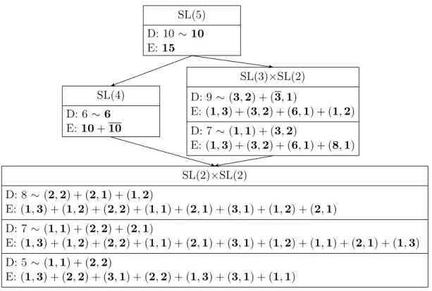
SL(5) D: 10∼10
E:15
SL(4) D: 6 ∼6
E:10+10
SL(3)×SL(2) D: 9 ∼(3,2) + (3,1)
E:(1,3) + (3,2) + (6,1) + (1,2) D: 7 ∼(1,1) + (3,2)
E:(1,3) + (3,2) + (6,1) + (8,1) SL(2)×SL(2)
D: 8 ∼(2,2) + (2,1) + (1,2)
E:(1,3) + (1,2) + (2,2) + (1,1) + (2,1) + (3,1) + (1,2) + (2,1) D: 7 ∼(1,1) + (2,2) + (2,1)
E:(1,3) + (1,2) + (2,2) + (1,1) + (2,1) + (3,1) + (1,2) + (1,1) + (2,1) + (1,3) D: 5 ∼(1,1) + (2,2)
E:(1,3) + (2,2) + (3,1) + (2,2) + (1,3) + (3,1) + (1,1)
Figure 1: Solutions of the linear constraints (C1) and (C2). “D:” lists the dimension of the group manifold and the corresponding coordinate irreps. All components of the embedding tensor which are in the kernel of the linear constraints are denoted by “E:”.
in seven dimensions [28], we know that also gaugings in the dual 40 are consistent. How do we resolve this contradiction? First, we implement the components of this irrep in terms of the tensor Zab,c and connect it to the40a, we discussed above, through
(X40a)a1a2,b1b2,c1c2c3 =a1a2d1d2[b1Z
d1d2,e1
b2]c1c2c3e1 (2.66) with the expected property
P40a(X40a)a1a2,b1b2,c1c2c3 = (X40a)a1a2,b1b2,c1c2c3. (2.67) Following the argumentation in [28], we interpret Zab,c as a 10×5 matrix and calculate its rank
s= rank(Zab,c). (2.68)
The number of massless vector multiplets in the resulting seven-dimensional gauged supergravity is given by 10−s. They contain the gauge bosons of the theory and transform in the adjoint representation of the gauge groupG. Thus, we immediately deduce
dimG= 10−s . (2.69)
compactification is in one-to-one correspondence with the group manifold we are considering [54]. There is no reason why it should be different for gEFT. So, if we switch on gaugings in the 40, we automatically reduce the dimension of the group manifold representing the extended space. Possible ranks s which are compatible with the quadratic constraint of the embedding tensor are 0 ≤ s ≤ 5. For those cases we have to adapt the coordinates on the group manifold. To this end, we consider possible branching rules of SL(5) to its U-/T-duality subgroups given in table 1, e.g. SL(4), SL(3)×SL(2) and SL(2)×SL(2)
10→4+6 (2.70)
10→(1,1) + (3,2) + (3,1) (2.71)
10→(1,1) + (1,1) + (2,1) + (1,2) + (2,2). (2.72) For the first one, we obtain a six-dimensional manifold whose coordinates are identified with the
6 of the branching rule (2.70) after dropping the 4. In the adapted basis
V4 ={15,25,35,45} V6 ={12,13,14,23,24,34} (2.73)
V4 ={234,134,124,123} V6 ={345,245,235,145,135,125}, (2.74) σ2 is now restricted to
σ2 :V6×V6×V6 →V6×V6×V6×V6×V6, (2.75)
while the irreps 15and 40split into
15→
S1+S4+10 (2.76)
40→
AA
4+6+10 +H20H. (2.77)
All crossed out irreps at least partially depend on V4 or its dual which is not available as coordinate irrep anymore. Of course, the10from the15still satisfies all linear constraints. But now only the 6 is excluded by the second linear constraint (2.64) with (2.75), while the 10 is in its kernel. This result is in alignment with the SL(4) case we discuss in appendix A. Hence, switching on specific gaugings in the 40 breaks indeed the U-duality group into a subgroup. An alternative approach [38] is to keep the full SL(5) covariance of the embedding tensors by not solving the linear constraints. However this technique obscures the interpretation of the extended space as a group manifold which is crucial for constructing the generalized frame EA
2.5 Quadratic Constraint
Finally, we come to the quadratic constraint (2.36) which simplifies drastically to
X[BC]EX[ED]A+X[DB]EX[EC]A+X[CD]EX[EB]A= 0 (2.78) after solving the linear constraints which result in ZCAB = 0 for the remaining coordinates on
the group manifold G. Now, it is identical to the Jacobi identity (2.40) which is automatically fulfilled for the Lie algebrag. Thus, the flat derivative satisfies the first Bianchi identity (2.39). For the covariant derivative (2.33), we compute the curvature and the torsion by evaluating the commutator
[∇A,∇B]VC =RABCDVD−TABD∇DVC. (2.79)
Doing so, we obtain the curvature
RABCD = 2Γ[A|CEΓ|B]ED+X[AB]EΓECD, (2.80)
where we used that ΓABC is constant due to (2.35) and the torsion
TABC =−X[AB]C + 2Γ[AB]C =YCD[A|EΓD|B]E, (2.81) for which we used (2.35) and (2.38). In general both are non-vanishing. Using these equations, we can compute the first Bianchi identity
R[ABC]D+∇[ATBC]D −T[ABETC]ED =
2X[AB]EX[CE]D+ 2X[CA]EX[BE]D+ 2X[BC]EX[AE]D = 0 (2.82) for ∇. Again, it is fulfilled because of the Jacobi identity (2.40). These results are in agreement with DFTWZW. It is straightforward to check that all gaugings, given in table 3 of [28], can be reproduced in the framework we presented in the first part of this paper. Explicit examples with with ten-dimensional groups CSO(1,0,4)/SO(5) and also a nine-dimensional group are discussed in section4.
3 Section Condition Solutions
the generalized tangent bundleT M⊕Λ2T∗M. Sometimes, the choice of the subgroup H is not unique for a given G. Different subgroups result in dual backgrounds. Section 3.4 presents a way to systematically study these different possibilities. It works exactly as in [49], so we keep the discussion brief. Starting from the SC solution, we construct the generalized frame field
EA fulfilling (1.2) in section 3.5. We also introduce the additional constraint on the structure
constantsXABC which is required for this construction to work.
3.1 Reformulation as H-Principal Bundle
Following the discussion in [49], we first substitute the quadratic version (2.23) of the SC by the equivalent linear constraint [3]
vaaBCDB·= 0 (3.1)
which involves a vector field va in the fundamental (SC irrep) of SL(5). This field can take
different values on each point ofG. In order to relate different points, remember that translations on G are generated by the Lie algebra g. Especially, we are interested in the action of its generators in the representations
5: (tA)bc=XA,bc and 10: (tA)BC =XABC = 2XA,[b1 [c1δ
b2]c2]= 2(tA)[b1 [c1δ
b2]c2]. (3.2) Both are captured by the embedding tensor. The corresponding group elements arise after apply-ing the exponential map. Now, assume we have a set of fields fi with a coordinate dependence
such that they solve the linear constraint (3.1) for a specific choice of va. Then, there exists
another set of fieldsfi0 with a different coordinate dependence
DAfi0 = (Adg)ABDBfi and (Adg)ABtB =g tAg−1 (3.3)
which solve the linear constraint after transformingva according to
v0a= (g)abvb. (3.4)
Here,(g)ab represents the left action of a group element gon the vectorvb. This property of the
linear constraint (3.1) is due to the fact that a totally anti-symmetric tensoris SL(5)invariant. The situation is very similar to the one in DFTWZW. Only the groups and their represen-tations are different. A minor deviation from [49] is the splitting of the 10indices into two sets of subindices. In order to implement the section condition, we introduce a vector va0 which gives rise to
v0aaβCtβ = 0 and va0a
˜
βCt
˜
β 6= 0. (3.5)
It splits the generatorstA ofg
tA=
tα tα˜
and tα ∈m, t˜α∈h (3.6)
va0 invariant under the transformation (3.4). This suggests to decompose each group element g∈Ginto
g=mh with h∈H (3.7)
while m is a coset representative of the left coset G/H. Because the action of h is free and transitive, we can interpretG as aH-principal bundle
π:G→G/H=M (3.8)
over M, the physical manifold.
We now study this bundle in more detail. The discussion is closely related to the one in [49]. So we keep it short, but still complete. A group elementg∈Gis parameterized by the coordinatesXI. In order to implement the splitting (3.6), we assign to the coset representativem
(generated bytα) the coordinatesxiand to the elementsh∈H(generated byt˜α) the coordinates
x˜i. Doing so, results in XI =
xi x˜i with I = 1, . . . , dimG , i= 1, . . . , dimG/H and ˜i= ˜1, . . . ,dimH . (3.9) In these adapted coordinates π acts by removing the x˜i part of the XI,
π(XI) =xi. (3.10)
We also note that the corresponding differential map reads
π∗(VI∂I) =Vi∂i. (3.11)
Each element of the Lie algebraggenerates a fundamental vector field onG. If we want to relate the two of them, we need to introduce the map
t]A=EAI∂I (3.12)
which assigns a left-invariant vector field to eachtA∈g. It has the important propertyωL(t]A) =
tA where
(ωL)g =g−1∂Ig dXI =tAEAIdXI (3.13)
is the left-invariant Maurer-Cartan form on G. Both (3.13) and (3.12) are completely fixed by the generalized background vielbein EAI and its inverse transposed EAI. After taking into
account the splitting of the generators (3.6) and the coordinates (3.9), they read
EAI =
Eαi 0
Eα˜i Eα˜˜i
!
and EAI =
Eαi Eα˜i
0 E˜α˜i
!
. (3.14)
We further equip the principal bundle with the h-valued connection one-form ω. It splits the tangent bundle T Ginto a horizontal/vertical bundle HG/V G. While the horizontal part
follows directly from the connection one-form, the vertical one is defined as the kernel of the differential map π∗. We have to impose the two consistency conditions
ω(t]α˜) =tα˜ and R∗hω=Adh−1ω (3.16) on ω, where Rg denotes right translations on G by the group element g ∈ G. In analogy to
DFTWZW the connection one-form is chosen such that the bundle HGsolves the linear version (3.1) of the SC. Following [49], we introduce the projectorPmat each pointmof the coset space
G/H as a map
Pm :g→h, Pm =tα˜(Pm)α˜BθB (3.17)
where we denote the dual one-form of the generator tA as θA. Pm is not completely arbitrary.
It has to have the property
Pmt˜α=t˜α ∀t˜α ∈h. (3.18)
So far, this projector is only defined for coset representativesmnot for arbitrary group elements g. But, we can extend it to the full group manifoldGby
Pg=Pmh= Adh−1PmAdh. (3.19) This allows us to derive the connection-one form
ωg =Pg(ωL)g (3.20)
where (ωL)g is the left-invariant Maurer-Cartan from (3.13). As a result of (3.18), it satisfies
the constraints in (3.16).
Finally, theH-principal bundle (3.8) has sectionsσi which are only defined in the patches
Ui ⊂M. They have the form
σi(xj) =
δkjxk fi˜j
(3.21) in the coordinates (3.9) and are specified by the functionsfi˜j. As for DFTWZW, we choose those functions such that the pull back of the connection one-form Ai =σi∗ω vanishes in every patch
Ui [49]. This is only possible if the corresponding field strength
Fi(X, Y) =dAi(X, Y) + [Ai(X), Ai(Y)] = 0 (3.22)
vanishes. In this case,Ai is a pure gauge and can be locally “gauged away”. It is very important
to keep in mind that this field strength is not the one that describes the tangent bundle T M. Take for example the four sphereS4 ∼=SO(5)/SO(4). It is not parallelizable and thus its tangent bundle cannot be trivial. However, this has nothing to do with the field strength defined in (3.22).
3.2 Connection and Three-Form Potential
For DFTWZW the projectorPm is related to the NS/NS two-form fieldBij. In the following we
solutions to the linear version of the SC (3.5) in more detail. By an appropriate SL(5) rotation, it is always possible to bringva0 into the canonical form
va0 =1 0 0 0 0
. (3.23)
This allows us to fix an explicit basis
α={12,13,14,15} and α˜ ={23,24,25,34,35,45} (3.24) for the indices appearing in our construction. Furthermore, we introduce the tensor
ηαβ,γ˜ = 1 2
1 ˆαβˆ˜γ (3.25)
whereβˆlabels the second fundamental index of the anti-symmetric pair (e.g. β= 13andβˆ= 3). The lowered version ofη is defined in the same way
ηαβ,˜γ=1 ˆαβˆ˜γ (3.26)
and its normalization is chosen such that the relations
ηαβ,α˜ηαβ,β˜ =δβα˜˜ and ηαβ,α˜ηγδ,α˜ =δ [α
[γδ β]
δ] (3.27)
are satisfied. Using this tensor, we express the projector (Pm)α˜B =
ηγδ,α˜Cβγδ δβα˜˜
(3.28) in terms of the totally anti-symmetric field Cαβγ on M. As we will see by considering the SC
solution’s GG in the next section, this field is related to the three-from flux C= 1
6CαβγE
α
iEβjEγkdxi∧dxj∧dxk (3.29)
on the background. Remember that the projector (3.28) is chosen such that its kernel contains all the solutions of the linear SC (3.1) for a fixedva. It is straightforward to identify
Cαβγ =
1 v1
X
δ
1 ˆαβˆγˆˆδvˆδ. (3.30)
However, this equation is only defined for v1 6= 0. Because (3.1) is invariant under rescaling all values of va specifying a distinct solution of the section condition are elements of RP4. This projective space has five patches Ua = {va ∈ R5|va = 1} in homogeneous coordinates. From
calculate the three-from flux C =−1
6ηαβ,˜γE
α
iEβjE˜γkdxi∧dxj ∧dxk (3.31)
which appears in the GG of the theory.
Again, it is a convenient crosscheck to consider the symmetry breaking from SL(5) to SL(4) which we discussed in section 2.4. Now, the index of va runs only from a = 1, . . . ,4 and the
linear constraint reads
v0aaβc= 0 (3.32)
with a four-dimensional totally anti-symmetric tensorand the explicit basis
α={12,13,14} and α˜={23,24,34}, (3.33) if we take v0a=1 0 0 0
. At this point, we have to restrict C from our previous discussion to the two-from
Cαβ4 =Bαβ (3.34)
in order the describe SC solutions with v5 = 0. Applying this restriction to (3.28) and (3.30) gives rise to
(Pm)α˜B =
ηγ,α˜Bβγ δαβ˜˜
and Bαβ =
1 v1
X
γ
1 ˆαβˆˆγvˆγ (3.35)
with
ηα,β˜ =αβ˜ and ηα,β˜ =αβ˜. (3.36) Here the normalization for the η-tensor is chosen such that the analog relations
ηα,α˜ηα,β˜=δαβ˜˜ and ηα,α˜ηβ,α˜ =δαβ (3.37)
to (3.27) hold. Furthermore, the same comments apply as above, but this time forRP3 instead of RP4. These results are in agreement with the ones for DFTWZW in [49]. Especially, theη-tensor gives rise the O(3,3) invariant metric
ηAB =AB = 0 η
α,β˜
ηβ,α˜ 0
!
(3.38)
with indices A,B in the coordinate irrep 6 ofsl(4). The only difference to [49] is that we use a different basis for the Lie algebra in which the off-diagonal blocksηα,β˜andηβ,α˜ are not diagonal. In general, it can get quite challenging to find the vanishing connection Ai=0 which is
required to solve the SC. However, if mand hin the decomposition (3.6) form a symmetric pair with the defining property
there is an explicit construction. It was worked out for DFTWZW in [49] and we adapt it to gEFT in the following. Starting point is the observation that the connectionA vanishes if
Cijk =−ηαβ,γ˜EαiEβjEγ˜k (3.40)
is totally anti-symmetric in the indicesi,j,k. We rewrite this condition as
2Cijk−Ckij−Cjki =Dijk= 0 (3.41)
and study it further. To this end, it is convenient to introduce the notation
(tA, tB, tC) = 2ηαβ,γ˜−ηγα,β˜−ηβγ,α˜ (3.42) which allows us to express (3.41) as
Dijk= (m−1∂im, m−1∂jm, m−1∂km) (3.43)
after taking into account that Eαi andEα˜i are certain components of the left-invariant
Maurer-Cartan form (3.13) with a section whereh is the identity element of H. Following [49], we use the coset representative
m= exp −f(xi)
(3.44) which gives rise to the expansion
m−1∂im=
∞
X
n=0 1
(n+ 1)![f, ∂if]n with [f, t]n= [f|[. . . ,{z [f}
ntimes
, t]. . .]]. (3.45)
Thus, we are left with checking that
Dijk=
∞
X
n1=0
∞
X
n2=0
∞
X
n3=0
1
(n1+ 1)! (n2+ 1)! (n3+ 1)!
([f, ∂if]n1,[f, ∂jf]n2,[f, ∂kf]n3) (3.46)
is zero under the restriction (3.39). To do so, let us first simplify the notation by the abbreviation
hn1, n2, n3iijk:= ([f, ∂if]n1,[f, ∂jf]n2,[f, ∂kf]n3) (3.47) and rearrange the terms in (3.46) which results in
Dijk =
∞
X
m=0
X
n1+n2+n3=m
hn1, n2, n3iijk
(n1+ 1)! (n2+ 1)! (n3+ 1)! =
∞
X
m=0
Sijkm . (3.48)
This expression is zero if Sm
ijk vanishes for all m. Therefore, it permits to do the calculation
order by order. Let us start with
It vanishes because (tA, tB, tC) only gives a contribution if two of its arguments are in m and
one is in h as it is obvious from the definition (3.42). Here all arguments are in m. The next order gives rise to
Sijkm = 1
2!(h1,0,0iijk+h0,1,0iijk+h0,0,1iijk) = 0 (3.50) and implements a linear constraint on the structure constants XABC. It is equivalent to
([t,m],m,m) + (m,[t,m],m) + (m,m,[t,m]) = 0 (3.51) where t denotes a generator in the algebra sl(5). Its components furnish the adjoint irrep 24. Note that the splitting of the flat coordinate indicesA intoα and α˜ singles out the direction va0 in (3.23). Thus, it break SL(5) to SL(4) with the branching
24→
S1+4+4+15 (3.52)
of the adjoint irrep. There is only one generator, corresponding to the crossed out irrep, which violates (3.51). In quadratic order, we find
Sijk2 = 1
4(h1,1,0iijk+h0,1,1iijk+h1,0,1iijk) + 1
6(h2,0,0iijk+h0,2,0iijk+h0,0,2iijk) = 0 (3.53) which represents a quadratic constraint on the structure constants. A solution is given by the symmetric pair (3.39). It implies that the first three terms are of the form (h,h,m) plus cyclic permutations, while the last three terms are covered by(m,m,m). As noticed before, all of them vanish independently. More generally, we now have
[f, ∂if]n⊂
(
h nodd
m neven (3.54)
which implies
hn1, n2, n3iijk= 0 if n1mod 2 +n2mod 2 +n3mod 2 = 1. (3.55)
Take any contributionhn1, n2, n3iijk toSmijk in (3.48) which is governed byn1+n2+n3 =m. If m is even then either two of the integers n1, n2, n3 are odd while the third one is even, or they are all even. In both caseshn1, n2, n3iijk vanishes and so does the completeSm for evenm.
In combination with (3.54), (3.51) becomes
hn1+ 1, n2, n3iijk+hn1, n2+ 1, n3iijk+hn1, n2, n3+ 1iijk= 0 forn1, n2, n3 even. (3.56)
We use this identity to simplify the cubic contribution Sijk3 =−1
which is equivalent to (3.56) after substituting 1 with 3. Repeating this procedure again and again forSijkm with oddm, we finally obtain the conditions
hn1+ 2l+ 1, n2, n3iijk+hn1, n2+ 2l+ 1, n3iijk+hn1, n2, n3+ 2l+ 1iijk= 0 ∀ l∈N (3.58) (again with n1, n2, n3 even) for the desired result (3.41) which proves Ai=0. Proving them,
requires a generalization of (3.51) and exploits that the generatortin this equation is an element of m. As a consequence, the commutator relations of the symmetric pair (3.39) restrict tto the
4 and 4 in the decomposition (3.52). So we see that (3.51) is not an independent constraint, but follows directly from having a symmetric pair. Denoting the two remaining, dual irreps as xi and yi, wherei= 1, . . . , 4, the relation
[t, ∂it]2l+1 = [t, ∂it]1
xiyi
4
l
(3.59) holds. It reduces (3.58) to (3.56) and completes the prove. Finally, note that there is another case
[m,m]⊂m (3.60)
for which one immediately has a flat connection. It implies that all terms in (3.48) are of the form (m,m,m) and vanish.
3.3 Generalized Geometry
All solutions of the SC which we discussed in the last two subsections are closely related to GG. In order to make this connection manifest, we have to introduce a map betweenhand the vector space of two-forms Λ2Tp∗M at each pointp ∈ M. More specifically, we use the η-tensor (3.25) to define the bijective map ηp :h→Λ2Tp∗M as
ηp(t˜γ) =
1
2 ηαβ,˜γE
α
iEβjdxi∧dxj
σ(p) .
(3.61) Its inverse
η−p1(ν) = ηαβ,γ˜t˜γιEαιEβν
σ(p) (3.62)
follows form the properties of the η-tensors and the vectors Ea = Eai∂i. With this map and
π∗ (3.11), ωg(X) (3.20) from section 3.1, we are able to construct the generalized frame field
[23,29,33]
ˆ
EA(p) =π∗p(tA] ) +ηpωσ(p)(t
]
A) (3.63)
at each point p of the physical spaceM. It is a map from a Lie algebra element tAto a vector
in the generalized tangent space TpM ⊕Λ2Tp∗M of M at p. Note that we suppress the index
labeling the patch dependence of the section for the sake of brevity. However, the generalized frame field EˆA depends explicitly on the section. For a non-trivial H-principal bundle, we find
Using the properties of the maps
π∗(t]α˜) = 0, ωσ∗=σ∗ω=A= 0, π∗σ∗= idT M and ω(tα]˜) =tα˜, (3.64) we deduce the dual frame
ˆ
EA(p, v,v˜) =θA
ηp−1(˜v) +ισ∗p(v)(ωL)σ(p)
. (3.65)
Here, we denote elements of the generalized tangent bundle as V = v+ ˜v with v ∈ T M and ˜
v∈Λ2T∗M. Finally, let us expand the generalized frame and its dual into components
ˆ EA=
Eαi∂i+CαβγEβiEγjdxi∧dxj
ηβγ,α˜EβiEγjdxi∧dxj
!
and EˆA(v,˜v) = E
α ivi
ηβγ,α˜(E
βiEγjv˜ij−CβγδEδivi)
!
(3.66) where the dependence onp is understood and the indices labeling the patch are suppressed. In the calculation for the dual frame, one has to take into account
θα˜ωL(σ∗v)
=−Cβγδηγδ,α˜Eβivi (3.67)
which results fromσ∗ω= 0. This result makes perfect sense, because it reproduces the canonical vielbein of a SL(5) theory [29]
VAˆIˆ= Eαi EαkCijk
0 Eα[iEβj]
!
(3.68) and its inverse transposed. The Cijk in this expression is connected to the one we are using in
(3.67) by Cijk =CαβγEαiEβjEγk.
With the generalized frame and its inverse fixed, we are able to transport the generalized Lie derivative (2.32) to the generalized tangent bundle with the elements
VIˆ=
vi ˜vij
=VAEˆA
ˆ
I and the dual Vˆ I=
vi v˜ij
VAEˆAIˆ. (3.69) We distinguish the tangent bundle of the group manifold from the generalized tangent bundle by using hatted indices for the latter. In this index convention, (3.66) becomes
ˆ EA
ˆ
I= Eαi EαkCkij
0 ηij,α˜
!
and EˆAIˆ=
Eαi 0 −Cimnηmn,α˜ ηij,α˜
!
(3.70)
with
ηij,α˜ =ηβγ,α˜EβiEγj and ηij,α˜ =ηβγ,α˜EβiEγj. (3.71)
Employing the dual frame on the flat derivative, we obtain ∂Iˆ= ˆEAIˆDA=
∂i 0
. (3.72)
For the infinitesimal parameter of a generalized diffeomorphismξJˆ, we use the same convention
First, we have
b
LξV
ˆ
I=ξJˆ∂
ˆ
JV
ˆ
I−VJˆ∂
ˆ
Jξ
ˆ
I+YIˆJˆ
ˆ
KLˆ∂Jˆξ
ˆ
KVLˆ. (3.73)
Second, there is the curved versionFIˆJˆKˆ =F
ABCEˆAIˆEˆBJˆEˆCKˆ of FABC =X
ABC−LbEˆ
A ˆ EB
ˆ
IEˆC
ˆ
I. (3.74)
Together, they form the generalized Lie derivative
LξVIˆ=LbξV
ˆ
I+F
ˆ
JKˆ
ˆ
IξJˆVKˆ . (3.75)
In the following we show that Lbis the untwisted generalized Lie derivative of GG and FIˆJˆ
ˆ
K
implements its twist with the non-vanishing form and vector components
Fijkl
mn=Xα˜β˜γ˜ηij,α˜ηkl, ˜
βη mn,˜γ
Fijkl=Xαβ˜γEαiηjk,
˜
βE γl
Fijkl=X˜αβγηij,α˜EβkEγl
Fijk
lm =Fαβ˜γ˜Eαiηjk,
˜
βη
lm,˜γ+FijknClmn− FnojklmCino
Fijklm =Fαβ˜ γ˜ηij,α˜Eβkηlm,˜γ+FijknClmn− FijnolmCkno
Fijk=FαβγEαiEβjEγk− FilmkCjlm− FlmjkCilm
Fijkl =Fαβγ˜EαiEβjηkl,˜γ+FijmCklm− FimnklCjmn− FmnjklCimn+
FimnoC
jmnCklo+FmnjoCimnCklo− FmnopklCimnCjop (3.76)
with
Fαβγ=Xαβγ−fαβγ Fαβ˜γ=Xαβ˜γ−GijklEαiEβjηkl,γ˜
Fαβ˜˜γ=Xαβ˜γ˜+ 2fαβγηδγ,β˜ηδβ,˜γ Fαβ˜ ˜γ=−Fβα˜γ˜+fαγδηβδ,α˜ηαγ,˜γ. (3.77) Here
fαβγ= 2E[αi∂iEβ]jEγj and G=dC =
1
4!Gijkldx
i∧dxj∧dxk∧dxl (3.78)
are the geometric and four-form fluxes induced by generalized frame (3.70).
To explicitly check thatLbis equivalent to the familiar generalized Lie derivative [33,55] of
exceptional GG, we calculate its components. The evaluation of the first two terms in (3.75) is straightforward. However, the term containing the Y-tensor is more involved. Therefore, we proceed componentwise and start with
YABCDEˆAiEˆBj =YαβCDEˆαiEˆβj = 0. (3.79)
Y-tensor components areYijkLˆMˆ which we evaluate now. To this end, we consider
YijkLˆMˆ =−δk[iEj]a5aBCEBLˆECMˆ (3.80) and use the dual generalized frame (3.70) to obtain the non-vanishing component
Yijklmn =−2δ[ikδj][mδn]l. (3.81)
Due to the symmetry of the Y-tensor, we are now able to compute the third term in (3.73) and obtain
YijkLˆMˆ∂kξ
ˆ
LVMˆ =∂
iξk˜vkj+∂jξkv˜ik−∂iξ˜jkvk−∂jξ˜kivk. (3.82)
Taking into account the first and the second term as well, we finally have
b
LξVIˆ=Lbξ
vi
˜ vij
!
= Lξv
i
Lξv˜ij−3vk∂[kξ˜ij]
!
, (3.83)
which is the generalized Lie derivative of exceptional GG [33,55].
As in subsection 3.2, we check our results by considering the restriction to the T-duality subgroup SL(4). In this case we have to modify the mapηp :h→Tp∗M, which is now defined as
ηp(tβ˜) = ηα,β˜Eαidxi
σ(p) , (3.84)
to take the different η-tensor (3.36) for this duality group into account. Repeating all the steps from above, we find the generalized frame
ˆ EA=
Eαi∂i+BαβEβidxi
ηβ,α˜Eβidxi
!
its dual EˆA(v,v˜) = E
α ivi
ηβ,α˜(Eβi˜vi−BβγEγivi)
!
(3.85)
and the generalized Lie derivative of GG. It has the form (3.75) with
b
LξV
ˆ
I =
b
Lξ
vi ˜ vi
!
= Lξv
i
Lξv˜i−2vk∂[kξ˜i]
!
(3.86)
and the twist in (3.74) which now has to be evaluated for the generalized frame in (3.85). After an appropriate change of basis this expression matches the one derived in [49].
3.4 Lie Algebra Cohomology and Dual Backgrounds
In general, the SC admits more than one solution. They arise from different choices ofva0in (3.5) and result in a distinguished splitting of the Lie algebragin the coset partmand the subalgebra h. One can always restore the canonical form ofva0 (3.23) by a SL(5) rotation. For this case the index assignment (3.24) remains valid and we only have to check whether the generatorst˜α form
Let us review the salient features of the construction. First, we only consider transformations in the coset SO(5)/SO(4)⊂ SL(5). All others, at most scaleva0 and thus leave the subalgebra h invariant. A coset element
TAB = exp(λ tAB) (3.87)
is generated by applying the exponential map to a so(5) generator t acting on the coordinate irrep 10. It modifies the embedding tensor according to
XAB0 C =TADT
BEXDEFTFC. (3.88)
We expand this expression in λto obtain
XAB0 C =XABC+λδXABC+λ2δ2XABC+. . . (3.89)
and read off the g-valued two-forms
cn=tC(δnXABC)θA∧θB. (3.90)
Only transformations withδnX
˜
αβ˜γ = 0are allowed. Otherwisehfails to be a subalgebra. Finally,
we have to check whether the restricted forms
cn=t˜γ(δnXα˜β˜γ˜)θα˜∧θ ˜
β (3.91)
are in the Lie algebra cohomology H2(h,h). If so, they give rise to a infinitesimal non-trivial deformation of h. Obstructions to the integrability of this deformation lie inH3(h,h).
3.5 Generalized Frame Field
A significant application of the formalism presented in this paper is to construct the frame fields
EAIˆ of generalized parallelizable manifolds M. In the following, we show that EA
ˆ
I =−M ABEˆB0
ˆ
I (3.92)
fulfills the defining equation (1.6) in the introduction if an additional linear constraint on the structure constants XABC holds. The derivation is done step by step starting with the frame
ˆ
EA0 Iˆ. It differs from (3.70) by using a three-fromC instead of C (see (1.8) in the introduction). So first, we calculate
XAB0 C =LbEˆ0
A ˆ
EB0 IˆE0CIˆ (3.93)
which has the non-trivial components
Xαβ0 γ=fαβγ Xαβ0 ˜γ=GijklEαiEβjηkl,γ˜
Xα0β˜˜γ= 2fαβγηδγ,β˜ηδβ,γ˜ Xαβ˜0 ˜γ=−X
0
βα˜˜γ−fαγδηβδ,α˜ηαγ,˜γ. (3.94) As before fαβγ denotes the geometric flux (3.78) and
is the field strength corresponding toC. In (3.92), EˆA0 Iˆ is twisted by the SL(5) rotation
MBAtA=m−1tBm= (Adm−1)BAtA (3.96) with the inverse transpose
tAMAB =mtBm−1. (3.97)
Next, we combine the two of them and evaluate XAB00 C =Lb
MADEˆ0D(MB
EEˆ0
E
ˆ
I)MC
FEˆ0FIˆ. (3.98)
It is convenient to write the result as
XAB00 C =XDE000 FMADMBEMCF with XAB000 C =X
0
ABC + 2T[AB]C +YCDEBTDAE (3.99)
and
TABC =−EˆA0
ˆ
I∂ˆ IM
D
BMDC. (3.100)
Taking into account the special form ofMBA in (3.96), this tensor can be calculated:
TABC =−EˆAiEDiXDBC =
−XαBC+ηδ,
˜
δC
αδXδB˜ C 0
. (3.101)
In the second step, we remember that for a SC solution the connection Avanishes. This allows us to identify EαiEβ˜i =−ηγδ,β˜Cαγδ. By plugging the solution forTABC into (3.99), we obtain
the non-vanishing components
Xα000˜β˜˜γ=−Xα˜β˜˜γ Xα000β˜γ=−Xαβ˜
γ X000
˜
αβγ =−X˜αβγ
Xα000β˜˜γ=−2Xαβ000 γηδγ,β˜ηδβ,γ˜ Xαβ000˜ ˜γ=−X
000
βα˜γ˜
Xαβ000 γ=−2Xαβγ+ 2Xα˜[βγCα]δηδ,α˜+fαβγ (3.102)
and
Xαβ000˜γ=−2Xαβγ˜ + 2Xγαα˜ηδβ,α˜ηγδ,˜γ−(2XγβδCδα−4XγαδCδβ)ηγ,γ˜−
2XαβγCδγηδ,˜γ+GijklEαiEβjηkl,˜γ (3.103)
after imposing the constraints
XAβ˜γ˜ =−2XAβγηδγ,β˜ηδβ,γ˜ and Xαγδηβδ,α˜ηαγ,˜γ= 0. (C3) At this point, (3.96) proves to be a good choice. Up to a sign, many components are already as we want them to be. This gets even better, if we take into account the explicit expression
for the geometric flux which results in
Xα000β˜˜γ=−Xαβ˜γ˜, Xαβ000˜ ˜γ=−Xαβ˜ ˜γ and Xαβ000 γ=−Xαβγ (3.105)
after imposing the constraints (C3). Finally, there is the last contribution (3.103) which should evaluate to −Xαβ˜γ. It requires an appropriate choice for the four-form
Gijkl=f(x1, x2, x3, x4)ijkl. (3.106)
Being the top-form on M, it only has one degree of freedom captured by the function f. With this ansatz, the last term in (3.103) becomes
GijklEαiEβjηlk,˜γ=fdet(Eρi)1 ˆαβˆˆγδˆηγδ,˜γ. (3.107) If we choose f = λdet(Eρi) for an appropriate, constant λ, the miracle happens and we find
Xαβ000γ˜ =−Xαβγ˜. The key to this result is that the structure constantsXABC are not arbitrary,
but severely constrained by the linear constraints (C1), (C2) and (C3). The first two are solved in section 2.4and we present the solutions to the remaining one at the end of this section. For the moment, we continue with
XAB000 C =−XABC under (C1) - (C3). (3.108)
Structure constants of a Lie algebra are preserved under the adjoint action (3.96). Thus, we immediately imply
XAB00 C =XAB000 C =−XABC. (3.109)
Up to the minus sign, this is exactly the result we are looking for. In order to get rid of this wrong sign, we introduce an additional minus in the generalized frame field EAIˆ (3.92). The
result is equivalent to (1.8) in the introduction. As argued above, the three-from C it contains has to be chosen such that
G=dC=λdet(Eρi)dx1∧dx2∧dx3∧dx4=λvol, (3.110)
wherevolis the volume form on M induces by the frame field Eαi.
Finally, we have to find the solutions of the linear constraint (C3). Otherwise the construc-tion above does not apply. In order to identify these soluconstruc-tions, we discuss embedding tensor components in the 15[28]
Xabcd=δd[aYb]c (3.111)
parameterized by the symmetric matrix Yab and in the 40[28]
Xabcd=−2abcefZef,d (3.112)
![Table 1: U-duality groups [9] which have the T-duality groups O(d-1,d-1) as subgroup. More- More-over, the coordinate and section condition irreps [2, 3] of the corresponding EFTs [4–8, 13, 14]](https://thumb-us.123doks.com/thumbv2/123dok_us/8294140.2196441/3.892.115.774.202.315/table-duality-duality-subgroup-coordinate-section-condition-corresponding.webp)