arXiv:1602.00869v1 [math.ST] 2 Feb 2016
DOI:10.3150/14-BEJ686
Non-Gaussian semi-stable laws arising in
sampling of finite point processes
RITWIK CHAUDHURI* and VLADAS PIPIRAS**
1
Department of Statistics and OR, UNC-CH, Chapel Hill, NC 27599, USA. E-mail:*
A finite point process is characterized by the distribution of the number of points (the size) of the process. In some applications, for example, in the context of packet flows in modern communication networks, it is of interest to infer this size distribution from the observed sizes of sampled point processes, that is, processes obtained by sampling independently the points of i.i.d. realizations of the original point process. A standard nonparametric estimator of the size distribution has already been suggested in the literature, and has been shown to be asymp-totically normal under suitable but restrictive assumptions. When these assumptions are not satisfied, it is shown here that the estimator can be attracted to a semi-stable law. The assump-tions are discussed in the case of several concrete examples. A major theoretical contribution of this work are new and quite general sufficient conditions for a sequence of i.i.d. random variables to be attracted to a semi-stable law.
Keywords:domain of attraction; finite point process; sampling; semi-stable law
1. Introduction
We first explain the motivation behind this work, namely, understanding statistical prop-erties of certain estimators arising when sampling finite point process. The issues raised in the motivation require developing new theoretical results on the domain of attraction of the so-called semi-stable laws. We conclude this section by describing this theoretical contribution, along with the structure of this work.
LetW, W(i),i= 1,2, . . . , N, be i.i.d. integer-valued random variables with the
probabil-ity mass function (p.m.f.)fW(w),w≥1. Let also Bin(n, q) denote a binomial distribution with parameters n≥1, q∈(0,1). Consider random variables Wq, Wq(i), i= 1,2, . . ., N,
obtained from W, W(i), i= 1,2, . . . , N, through the relationships Wq = Bin(W, q) and
Wq(i)= Bin(W(i), q), i= 1,2, . . . , N (independently acrossi). Note thatWq takes values
in 0,1,2, . . ., W. Let the probability mass function ofWq befWq(s),s≥0. The basic
in-terpretation ofWq is as follows. If an object consists ofW points (a finite point process)
This is an electronic reprint of the original article published by theISI/BSinBernoulli,
2016, Vol. 22, No. 2, 1055–1092. This reprint differs from the original in pagination and typographic detail.
and each point is sampled with a probability q, then the number of sampled points is
Wq= Bin(W, q).
One application of the above setting arises in modern communication networks. A finite point process (an object) is associated with the so-called packet flow (and a point is associated with a single packet). Sampling is used in order to reduce the amount of data being collected and processed. One basic problem that has attracted much attention recently is the inference offW from the observed sampled data Wq(i), i= 1,2, . . . , N (in
principle,Wq(i)= 0 is not observed directly, but the inference about the number of times Wq(i)= 0 is made through other means). See, for example, Duffield, Lund and Thorup
[7], Hohn and Veitch [9], Yang and Michailidis [14]. For other, more recent progress on sampling in communication networks, see Antunes and Pipiras [2, 3], and references therein.
We are interested here in some statistical properties of a nonparametric estimator of
fW(w), introduced in Hohn and Veitch [9] and also considered in Antunes and Pipiras [1]. We first briefly outline how the estimator is derived. Estimation offW(w) is based on a theoretical inversion of the relation
fWq(s) = ∞
X
w=s
P(Wq=s|W =w)P(W=w)
(1.1)
=
∞
X
w=s
w s
qs(1−q)w−sfW(w), s≥0.
In terms of the moment generating functions GWq(z) =
P∞
s=0zsfWq(s) and GW(z) =
P∞
w=1zwfW(w), the relation (1.1) can be written asGWq(z) =GW(zq+ 1−q). By
chang-ing the variableszq+ 1−q=x, one hasGW(x) =GWq(q
−1x−q−1(1−q)) which has the
earlier form but withq replaced byq−1 (andz replaced byx). This suggests that (1.1)
can be inverted as
fW(w) =
∞
X
s=w
s w
(q−1)w(1−q−1)s−wfWq(s)
(1.2)
=
∞
X
s=w
s w
(−1)s−w qs (1−q)
s−wfW
q(s), w≥1.
Antunes and Pipiras [1], Proposition 4.1, showed that the inversion relation (1.2) holds when
∞
X
s=n
s n
(1−q)s−n
qs fWq(s) = ∞
X
w=n
w n
2w−n(1−q)w−nfW(w)<∞, n≥1. (1.3)
In view of (1.2), a natural nonparametric estimator offW is
b
fW(w) =
∞
X
s=w
s w
(−1)s−w qs (1−q)
s−wfWb
q(s), w≥1, (1.4)
where
b
fWq(s) =
1
N N
X
i=1
1{W(i)
q =s}, s≥0, (1.5)
is the empirical p.m.f. offWq, and 1Adenotes the indicator function of an eventA. Note
that, by using (1.4) and (1.2),
√
N(fWb (w)−fW(w)) =
∞
X
s=w
s w
(−1)s−w qs (1−q)
s−w√N(fWb
q(s)−fWq(s)). (1.6)
Since
{√N(fWb q(s)−fWq(s))} ∞ s=0
d
→{ξ(s)}∞s=0, (1.7)
where{ξ(s)}∞
s=0 is a Gaussian process with zero mean and covariance structure
E(ξ(s1)ξ(s2)) =fWq(s1)1{s1=s2}−fWq(s1)fWq(s2),
one may naturally expect that under suitable assumptions, (1.6) is asymptotically normal in the sense that
{√N(fWb (w)−fW(w))}∞w=1
d
→{S(ξ)w}∞w=1, (1.8)
where{S(ξ)w}∞
w=1 is a Gaussian process. Antunes and Pipiras [1], Theorem 4.1, showed
that (1.8) holds indeed ifRq,w<∞, w≥1, where
Rq,w=
∞
X
s=w
s w
2
(1−q)2(s−w)
q2s fWq(s)
(1.9)
=
∞
X
i=w
fW(i)(1−q)i−2w
i w
Xi
s=w
s w
i−w s−w
(q−1−1)s.
The quantity Rq,w is naturally related to the limiting variance of √NfWb (w). Indeed, since N E(fWb q(s1)−fWq(s1))(fWb q(s2)−fWq(s2)) =fWq(s1)1{s1=s2}−fWq(s1)fWq(s2)
and by using (1.6) and (1.2), the asymptotic variance of √NfWb (w) is expected to be
Rq,w−(fW(w))2. RequiringRq,w<∞is then a natural assumption in proving (1.8).
Section 4 below that if fW(w) = (1−c)cw−1, w≥1, is a geometric distribution with
parameterc∈(0,1), then the distribution offWq(s) is given by
fWq(s) =
(1−q)(1−c)
1−c(1−q) , ifs= 0, 1
cc s
q(1−cq), ifs≥1,
(1.10)
wherecq=1−ccq(1−q). Moreover, the conditionRq,w<∞holds if and only ifc <1−qq (see Section4). Thus, for example, we are interested what happens withfWb (w) whenWq has p.m.f. given by (1.10) withc≥1−qq.
To understand what happens whenRq,w=∞, observe from (1.4) and (1.5) thatfWb (w) can also be written as
b
fW(w) = 1
N N
X
i=1
Xi, (1.11)
whereXi,i= 1,2, . . . , N, are i.i.d. random variables defined as
Xi=
Wq(i) w
(−1)Wq(i)−w qWq(i)
(1−q)Wq(i)−w1
{Wq(i)≥w}. (1.12)
Focus on the key term (1−q)W
(i) q
qWq(i) = (q
−1−1)Wq(i) entering (1.12). For example, whenW
is geometric with parameterc,Wq(i) has p.m.f. in (1.10). One then expects that
P((q−1−1)Wq(i)> x) =P
Wq(i)>
logx
log(q−1−1)
(1.13)
≈1cclogq x/log(q−1−1)=
1
cx −α,
whereα= logc−
1 q
log(q−1−1). This suggests that the distribution ofXi,i= 1,2, . . . , N, has heavy
tail and that the estimatorfWb (w) is asymptotically non-Gaussian stable whenα <2. In fact, the story turns out to be more complex. Because of the discrete nature ofWq(i), the
relation (1.13) does not hold in the asymptotic sense asx→ ∞. An appropriate setting in this case involves the so-called semi-stable laws. In the semi-stable context, moreover, the convergence of (1.11) is expected only along subsequences ofN.
subsequence and after suitable normalization and centering). A common example (and, in fact, one of the few concrete examples) of such a distribution is that of a log-geometric random variable
X=aWq withP(Wq=s) = (1−cq)cs
q, s= 0,1, . . . , (1.14)
where a >0 and cq∈(0,1). (Strictly speaking, the log-geometric case is when a=e.) Note that in (1.14), we use purposely the notation of (1.10) and (1.12).
In fact, motivated by (1.12) and the desire to consider more general distributions than log-geometric, we will show that the domain of attraction of semi-stable laws also includes the distributions of random variables of the form
X=k(Wq)aWq withP(Wq=s) =h(s)cs
q, s= 0,1, . . . , (1.15)
wherekandhare functions satisfying suitable but also flexible conditions. Our approach goes through verifying that the distributions determined by (1.15) satisfy the necessary and sufficient conditions to be attracted to a semi-stable law. Somewhat surprising per-haps, the proof turns out to be highly nontrivial. The difficulty lies in dealing with the general case when both functionskandhin (1.15) are not constant. Much of this work, in fact, concerns this problem.
The rest of this work is structured as follows. Preliminaries on semi-stable laws can be found in Section2. In Section3, we state and prove the main general results of this work concerning semi-stable distributions and their domains of attraction. In Section4, we apply the main results from Section 3 to sampling of finite point processes. Several concrete examples, in particular, are considered. A few auxiliary results are given in the Appendix. Some numerical illustrations can be found in Chaudhuri and Pipiras [5].
2. Preliminaries on semi-stable laws
One way to characterize a semi-stable distribution is through its characteristic function (Maejima [11]).
Definition 2.1. A probability distributionµon R(or a random variable with distribu-tion µ) is called semi-stable if there existr, b∈(0,1) andc∈R such that
b
µ(θ)r=µb(bθ)eicθ for allθ∈R, (2.1)
andµb(θ)6= 0, for allθ∈R, whereµb(θ) denotes the characteristic function of µ.
A semi-stable distribution is known to be infinitely divisible (Maejima [11]) with a location parameterη∈R, a Gaussian part with varianceσ2≥0 and a non-Gaussian part
with L´evy measure characterized by (distribution) functions
L(x) =ML(x)
|x|α , x <0, R(x) =− MR(x)
whereα∈(0,2),ML(c1/αx) =ML(x) whenx <0, andMR(c1/αx) =MR(x) whenx >0,
for somec >0. The functionsML andMR are thus periodic with multiplicative period
c1/α. The functionsL(x) andR(x) are left-continuous and non-decreasing on (−∞,0) and
right-continuous and non-decreasing on (0,∞), respectively. The characteristic function of a semi-stable distribution with a location parameterη and without a Gaussian part is given by
logµb(t) = iηt+
Z 0
−∞
eitx−1−1 +itxx2
dL(x) +
Z ∞
0
eitx−1−1 +itxx2
dR(x). (2.3)
Semi-stable distributions arise as limits of partial sums of i.i.d. random variables. Let
X1, X2, . . .be a sequence of i.i.d. random variables with a common distribution function
F. Consider the sequence of partial sums
S∗ n=
1
Akn
(kn
X
j=1
Xj−Bkn
)
, (2.4)
where{Akn}and{Bkn}are normalizing and centering sequences. Semi-stable laws arise
as limits of partial sumsSn∗, supposing that{kn}satisfies
kn→ ∞, kn≤kn+1, lim
n→∞ kn+1
kn =c∈[1,∞). (2.5)
Moreover, ifS∗
nconverges to a nontrivial limit (semi-stable distribution), the distribution F ofXj is said to be in the domain of attraction of the limiting semi-stable law. In this case and supposing the limiting law is non-Gaussian semi-stable, it is known that the normalizing sequence{Akn} necessarily satisfies
Akn→ ∞, Akn≤Akn+1, lim n→∞
Akn+1 Akn
=c1/α whereα∈(0,2). (2.6)
Megyesi [13], Grinevich and Khokhlov [8] gave necessary and sufficient conditions for a distribution to be in the domain of attraction of a semi-stable distribution.
Theorem 2.2 (Megyesi [13], Corollary 3). Distribution F is in the domain of at-traction of a non-Gaussian semi-stable distribution with the characteristic function (2.3) along the subsequence kn with normalizing constants Akn satisfying (2.5) and (2.6) if and only if for allx >0 large enough,
F−(−x) =x−αl∗(x)(ML(−δ(x)) +hL(x)), (2.7)
1−F(x) =x−αl∗(x)(MR(δ(x)) +hR(x)), (2.8)
where l∗ is a right-continuous function, slowly varying at ∞, α∈(0,2),F
− is the left-continuous version of F and the error functions hR andhL are such that
for every continuity point x0 of MR, if K=R, and −x0 of ML, if K=L. MK, K∈
{L, R}, are two periodic functions with common multiplicative period c1/α and for all large enough x,δ(x)is defined as
δ(x) = x
a(x)∈[1, c
1/α+ε], (2.10)
whereε >0 is any fixed number, with
a(x) =Akn if Akn≤x < Akn+1. (2.11)
Grinevich and Khokhlov [8] also showed that, in the sufficiency part of the theorem above,kn can be chosen as follows. First, choose a sequence{An}˜ such that
lim
n→∞n
˜
A−α
n l∗( ˜An) = 1 (2.12)
and
˜
An→ ∞, An˜ ≤An˜ +1 and lim
n→∞
˜
An+1
˜
An = 1. (2.13)
Define a new sequence{an}by settingan=Aknfor everyn, whereAknappears in (2.11).
Then, the natural numberskn can be chosen as
˜
Akn≤an<Ak˜ n+1. (2.14)
The centering constantsBkn in (2.4) can be chosen as (Cs¨org¨o and Megyesi [6])
Bkn=kn
Z 1−1/kn
1/kn
Q(s) ds, (2.15)
where, for 0≤s≤1,
Q(s) = inf
y {F(y)≥s}. (2.16)
The location parameterη of the limiting semi-stable law in (2.3) is then given by
η= Θ(ψ1)−Θ(ψ2), (2.17)
where
Θ(ψi) =
Z 1
0
ψi(s) 1 +ψ2
i(s)
ds−
Z ∞
1
ψ3
i(s)
1 +ψ2
i(s)
ds, i= 1,2, (2.18)
and
ψ1(s) = inf
x<0{L(x)> s}, ψ2(s) = infx<0{−R(−x)> s}. (2.19)
It is also worth mentioning that the slowly varying functionl∗(x) entering in (2.7) and
(2.8) can be replaced by two different, asymptotically equivalent slowly varying functions
l∗
3. General results concerning semi-stable domain of
attraction
The next theorem is the main result of this work. We use the following notation through-out this work:
⌈x⌉= the smallest integer larger than or equal tox, ⌈x⌉+= the smallest integer strictly larger thanx.
For example, ⌈2.47⌉=⌈2.47⌉+= 3 but ⌈3⌉= 3 and ⌈3⌉+= 4. The function ⌈x⌉+ is the
right-continuous version of the function⌈x⌉. Also note that ⌈x⌉+= [x] + 1, where [x] is
the integer part ofx(i.e., the largest integer smaller than or equal tox).
Theorem 3.1. Let Wq be an integer-valued random variable taking values in 0,1,2, . . . such that, for allx >0,
P
Wq
2 ≥x, Wq is even
=
∞
X
n=⌈x⌉ P
Wq
2 =n
=h1(⌈x⌉)e−ν⌈x⌉, (3.1)
P
Wq−1
2 ≥x, Wq is odd
=
∞
X
n=⌈x⌉ P
Wq−1
2 =n
=h2(⌈x⌉)e−ν⌈x⌉, (3.2)
whereν >0 and the functionsh1 andh2 satisfy
h2(x)
h1(x)→c1 asx→ ∞, (3.3)
for some fixedc1≥0, and
h1(ax)
h1(x) →1 asx→ ∞, a→1. (3.4)
Let also
X=L(eWq)eβWq(−1)Wq, (3.5)
where β >0 and L is a slowly varying function at ∞ such that L(en) is ultimately monotonically increasing. Suppose that
α:= ν
2β <2. (3.6)
Then, X is attracted to the domain of a semi-stable distribution in the following sense. If X, X1, X2, . . .are i.i.d. random variables, then as n→ ∞, the partial sums
1
Akn
(kn
X
j=1
Xj−Bkn
)
converge to a semi-stable distribution with
kn=
e(n−1)ν
h1(n−1)
, Akn=L(e
2n−2)e2β(n−1) (3.8)
andBkn given by (2.15). The limiting semi-stable distribution is non-Gaussian, has lo-cation parameter given in (2.17) and is characterized by
α= ν
2β, (3.9)
ML(−x) =c1e−ν([1/2+(1/(2β)) logx]−(1/(2β)) logx),
(3.10)
MR(x) = e−ν(⌈(1/(2β)) logx⌉+−(1/(2β)) logx), x >0.
Proof. The result will be proved by verifying the sufficient conditions (2.7)–(2.8) of Theorem2.2. We break the proof into two cases dealing with (2.7) and (2.8) separately. The final part of the proof shows that the sequencekn can be chosen as in (3.8).
Step 1 (showing (2.8)): Fixx >0 large enough. In view of (3.5), we are interested in
¯
F(x) := 1−F(x) =P(L(eWq)eβWq(−1)Wq> x). (3.11)
LetZ2=W2q. Note that (3.11) can be written as
¯
F(x) =P(L(e2Z2)e2βZ2> x, Z
2is integer)
=P(L(e2Z2)e2βZ2> x) (3.12)
=P
Z2+
1
2βlogL(e
2Z2)> 1
2βlogx
,
where, in view of (3.1),
P(Z2≥x) =h1(⌈x⌉)e−ν⌈x⌉. (3.13)
We next want to write ¯F(x) in (3.12) as
¯
F(x) =P
Z2≥g
1 2βlogx
(3.14)
for some functiong.
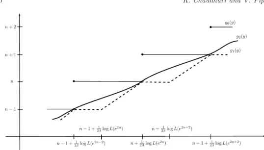
There are many choices forg in (3.14). One natural choice is to take
g0(y) =n if (n−1) + 1
2βlogL(e
2n−2)
≤y < n+ 1
2βlogL(e
2n). (3.15)
The functiong0, however, turns out not to be suitable for our purpose. It will be used
Figure 1. Plot of g0(y),g1(y) andg2(y).
functiong1defined, for integer n≥2, as
g1(y) =
n−1,
ifn−1 + 1
2βlogL(e
2n−2)≤y < n−1 + 1
2βlogL(e
2n),
y−21βlogL(e2n),
ifn−1 + 1
2βlogL(e
2n)
≤y < n+ 1
2βlogL(e
2n).
(3.16)
We will also use the function
g2(y) =f−1(y) = inf{z: f(z)≥y} (3.17)
defined as an inverse of the function
f(z) =z+ 1
2βlogL(e
2z). (3.18)
Note that
⌈g0(y)⌉=⌈g1(y)⌉+=⌈g2(y)⌉+=⌈g(y)⌉, (3.19)
where g is any function satisfying (3.14). The functions g0, g1 and g2 are plotted in
We shall use another function ˜g1 which modifiesg1 in the following way: for n≥2,
˜
g1(y) =y− 1
2βlogL(e
2n−2)
(3.20) ifn−1 + 1
2βlogL(e
2n−2)
≤y < n+ 1
2βlogL(e
2n).
One relationship between the functions g1 and ˜g1 can be found in Lemma A.1 in the
Appendix, and will be used in the proof below. Note that ˜g1(y) can be expressed as
˜
g1(y) =y−˜g∗1(y), (3.21)
where, forn≥2,
˜
g∗1(y) =
1
2βlogL(e
2n−2) ifn
−1 + 1
2βlogL(e
2n−2)
≤y < n+ 1
2βlogL(e
2n). (3.22)
See Lemma A.2 in the Appendix for a property of ˜g∗
1 which will be used in the proof
below.
We need few properties of the functiong2. Sinceg2is the inverse of the functionf, we
have eg2(logx) as the inverse of ef(logx). Indeed,
eg2(log ef(logx))= eg2(f(logx))= elogx=x.
Note now from (3.18) that
ef(logx)= elogx+(1/(2β)) logL(x2)=x(L(x2))1/(2β).
Since (L(x2))1/(2β) is a slowly varying function, ef(logx) is a regularly varying function.
So, by Theorem 1.5.13 of Bingham, Goldie and Teugels [4],
eg2(logx)=xl(x),
wherel(x) is a slowly varying function. Hence,
g2(logx) = logx+ logl(x) = logx+g∗2(logx),
where
g∗
2(logx) = logl(x)
or replacing logxbyy,
g2(y) =y+g2∗(y). (3.23)
Note also that for anyA >0, we have
g∗2(logAx)−g2∗(logx) = logl(Ax)−logl(x) = log
l(Ax)
Continuing with (3.14) now, note that, by using (3.13) and (3.19),
¯
F(x) =P
Z2≥g
1 2βlogx
=h1
g
1
2βlogx
e−ν⌈g((1/(2β)) logx)⌉ (3.25)
=h1
g2
1 2βlogx
+
e−ν⌈g1((1/(2β)) logx)⌉+.
By using (3.21), note further that
¯
F(x) =h1
g2
1 2βlogx
+
e−ν˜g1((1/(2β)) logx)
×e−ν(g1((1/(2β)) logx)−˜g1((1/(2β)) logx))e−ν(⌈g1((1/(2β)) logx)⌉+−g1((1/(2β)) logx))
=h1
g2
1
2βlogx
+
e−ν((1/(2β)) logx−g˜1∗((1/(2β)) logx)) (3.26)
×e−ν(g1((1/(2β)) logx)−˜g1((1/(2β)) logx))e−ν(⌈g1((1/(2β)) logx)⌉+−g1((1/(2β)) logx))
=x−αl∗1(x)(MR(δ(x)) +hR(x)),
whereα= ν
2β as given in (3.9),
l1∗(x) =h1
g2
1
2βlogx
+
eν˜g1∗((1/(2β)) logx)
(3.27)
×e−ν(g1((1/(2β)) logx)−g˜1((1/(2β)) logx)),
MR(δ(x)) = e−ν(⌈g˜1((1/(2β)) logx)⌉+−g˜1((1/(2β)) logx)) (3.28)
and
hR(x) = e−ν(⌈g1((1/(2β)) logx)⌉+−g1((1/(2β)) logx))
(3.29)
−e−ν(⌈g˜1((1/(2β)) logx)⌉+−g˜1((1/(2β)) logx)).
We next show that the functionsl∗
1, MR and hR satisfy the conditions of Theorem2.2
with suitable choices ofδ(x) and Akn.
By LemmaA.3 in the Appendix, l∗
1(x) is a right-continuous slowly varying function
and hence it satisfies the conditions of Theorem2.2. For the function MR(δ(x)), note from (3.28) that
MR(δ(x)) = e−ν(⌈2βg˜1((1/(2β)) logx)/(2β)⌉+−2βg˜1((1/(2β)) logx)/(2β))
with
MR(x) = e−ν(⌈logx/(2β)⌉+−logx/(2β)). (3.31) The function MR(x) is periodic with multiplicative period e2β, and is right-continuous
as required in Theorem2.2. Since the period e2β is alsoc1/α, this yields
c= eν. (3.32)
To chooseδ(x), note from (3.30) that
MR(δ(x)) =MR(e2βg˜1((1/(2β)) logx)−2β(n−1)),
for anyn≥1, sinceMR has multiplicative period e2β. We can set
δ(x) = e2β˜g1((1/(2β)) logx)−2β(n−1) if e2β(n−1)L(e2n−2)≤x <e2nβL(e2n). (3.33)
From (3.20), we have
δ(x) = e2β((1/(2β)) logx−(1/(2β)) logL(e2n−2))−2β(n−1)
(3.34)
= x
e2β(n−1)L(e2n−2) if e
2β(n−1)L(e2n−2)
≤x <e2nβL(e2n).
Thus,δ(x) has the required form (2.10)–(2.11) with
Akn= e
2β(n−1)L(e2n−2) (3.35)
and
a(x) = e2β(n−1)L(e2n−2) =Ak
n ifAkn≤x < Akn+1. (3.36)
Note also from (3.34) that
1≤δ(x)< e
2βnL(e2n)
e2β(n−1)L(e2n−2)
= e2β L(e2n) L(e−2e2n)→e
2β=c1/α,
so thatδ(x)∈[1, c1/α+ε] for large enoughxwhenε >0 is fixed.
To complete step 1, we need to prove thathR(Aknx0)→0 as n→ ∞ for every
conti-nuity pointx0 ofMR(x). The discontinuity points ofMR are
x= e2kβ, k∈Z. (3.37)
To show hR(Aknx0)→ 0, note that, by Lemma A.1, it is enough to prove that
˜
hR(Aknx0)6= 0 for finitely many values ofn, where
˜
This holds only if for some integerm≥2,
m+ logL(e2m−2)≤21βlogAknx0< m+ logL(e
2m). (3.38)
By LemmaA.4, (3.38) holds for infinitely many values ofnonly ifx0= e2rβ,r∈Z, which
is a discontinuity point of MR(x) in (3.37). Hence, hR(Aknx0)→0 as n→ ∞ for every
continuity pointx0 ofMR(x).
Step 2 (showing (2.7)): In view of (3.5), we are now interested in
F−(−x) =P(L(eWq)eβWq(−1)Wq<−x). (3.39)
LetZ2=W2q as in step 1. Note that (3.39) can be written as
F−(−x) =P
L(e2Z2)e2βZ2> x, Z
2−
1
2 is integer
=P
L(ee2(Z2−1/2))eβe2β(Z2−1/2)> x, Z2−1
2 is integer
(3.40) =P(L(ee2Z1)eβe2βZ1> x)
=P
Z1+
1 2+
1
2βlogL(e
2Z1+1)> 1
2βlogx
,
where, in view of (3.2),
P(Z1≥x) =h2(⌈x⌉)e−ν⌈x⌉. (3.41)
Writing (3.40) as
F−(−x) =P
Z1+
1
2βlogL(e
2Z1+1)> 1
2βlogx−
1 2
,
the right-hand side has the form (3.11) whereL(e2Z2) is replaced byL(ee2Z1) and 1
2βlogx
is replaced by 1
2βlogx−
1
2. Thus, as in (3.14)–(3.15), one can write
F−(−x) =P
Z1≥g˜
1
2βlogx−
1 2
, (3.42)
where
˜
g(y) =n ifn−1 + 1
2βlogL(ee
2n−2)
≤y < n+ 1
2βlogL(ee
2n). (3.43)
The expression (3.42) can also be written as
F−(−x) =P
Z1≥g˜0
1 2βlogx
where ˜g0(y) = ˜g(y−12) or, forn≥2,
˜
g0(y) =n ifn−
1 2 +
1
2β logL(e
2n−1)
≤y < n+1 2 +
1
2βlogL(e
2n+1). (3.45)
We want to work with the intervals [n−1 +21βlogL(e2n−2), n+ 1
2βlogL(e2n))
ap-pearing in step 1, and use the results of that step. Note that, on the interval [n−1 +
1
2βlogL(e2n−2), n+
1
2βlogL(e2n)), the function ˜g0 has the form
˜
g0(y) =
n−1, ifn−1 + 1
2βlogL(e
2n−2)
≤y < n−12+ 1
2βlogL(e
2n−1),
n, ifn−12+ 1
2βlogL(e
2n−1)
≤y < n+ 1
2βlogL(e
2n). (3.46)
Defining
I0(y) =
−1, ifn−1 + 1
2βlogL(e
2n−2)
≤y < n−12+ 1
2βlogL(e
2n−1),
0, ifn−12+ 1
2βlogL(e
2n−1)
≤y < n+ 1
2βlogL(e
2n), (3.47)
and combining (3.15), (3.46) and (3.47), we have
˜
g0(y) =g0(y) +I0(y). (3.48)
Continuing with (3.44), note further that, by using (3.41) and (3.48),
F−(−x) =h2
˜
g0
1 2βlogx
e−ν˜g0((1/(2β)) logx)
(3.49) = e−νI0((1/(2β)) logx)h
2
g0
1 2βlogx
+I0
1 2βlogx
e−νg0((1/(2β)) logx).
We want to write F−(−x) as in (2.7) of Theorem 2.2 (where by Lemma A.5, we can
take a slowly varying functionl∗
2 which is asymptotically equivalent to l1∗). We need the
notation for the intervals appearing in (3.46)–(3.47), namely, forn≥1,
Dn=
n−1 + 1
2β logL(e
2n−2), n
−12+ 1
2βlogL(e
2n−1)
,
En=
n−1
2+ 1
2βlogL(e
2n−1), n+ 1
2βlogL(e
2n)
.
We also need a similar notation without the slowly varying functionL, that is, forn≥1,
D′
n= [n−1, n−12), E
′
Set also
D=
∞
[
n=1
Dn, E=
∞
[
n=1
En,
(3.50)
D′=
∞
[
n=1
D′n, E′= ∞
[
n=1
En′.
As in (3.26), we can now write (3.49) as
F−(−x) =x−αh2(g0((1/(2β)) logx) +I0((1/(2β)) logx)) c1h1(g0((1/(2β)) logx))
l1∗(x)c1e−νI0((1/(2β)) logx)
×e−ν(⌈g1((1/(2β)) logx)⌉+−g1((1/(2β)) logx)),
whereα= ν
2β andl ∗
1(x) is given in (3.27). This can also be written as
F−(−x) =x−αl∗2(x)(ML(−δ(x)) +hL(x)),
where
l2∗(x) =
h2(g0((1/(2β)) logx) +I0((1/(2β)) logx))
c1h1(g0((1/(2β)) logx))
l∗1(x), (3.51)
ML(−δ(x)) =c1e−ν([1/2+˜g1((1/(2β)) logx)]−˜g1((1/(2β)) logx)), (3.52)
hL(x) =c1e−νI0((1/(2β)) logx)e−ν(⌈g1((1/(2β)) logx)⌉+−g1((1/(2β)) logx))
(3.53)
−c1e−ν([1/2+˜g1((1/(2β)) logx)]−g˜1((1/(2β)) logx)).
By using (3.3)–(3.4), we have
h2(g0((1/(2β)) logx) +I0((1/(2β)) logx))
c1h1(g0((1/(2β)) logx)) →
1 asx→ ∞.
Hence, l∗2(x) l∗
1(x)→1, as x→ ∞, that is, l ∗
2(x) and l1∗(x) are two asymptotically equivalent
functions. By the definition of I0 and using LemmaA.3, l∗2(x) is right-continuous and
slowly varying.
The function δ(x) appearing in (3.52) is the same as in (3.33)–(3.34) of step 1, while the functionML(−x) is defined as
ML(−x) =c1e−ν([1/2+(1/(2β)) logx]−(1/(2β)) logx), x >0. (3.54)
It is left-continuous whenx >0, and also periodic with multiplicative period e2β=c1/α.
Thus,ML(x) for x <0 is left-continuous as required in Theorem 2.2. The discontinuity points ofML(−x) are
To conclude the proof of step 2, we need to show thathL(Aknx0)→0 asn→ ∞ for
every continuity pointx0ofML(−x), that is,x0different from (3.55). For this, we rewrite
hL(x) as follows. Observe that
e−νI0(y)= eν1
D(y) + 1E(y)
and
(eν1D′(y) + 1E′(y))e−ν(⌈y⌉+−y)= e−ν([1/2+y]−y),
where after taking the logs, using ⌈y⌉+= [y] + 1 and simplification, the last identity is
equivalent to [y]1D′(y) + ([y] + 1)1E′(y) = [12+y] and can be seen easily by drawing a picture. By using these identities and (3.53), we can write
c−11hL(x) =
eν1 D
1 2βlogx
+ 1E
1 2βlogx
e−ν(⌈g1((1/(2β)) logx)⌉+−g1((1/(2β)) logx))
−e−ν([1/2+˜g1((1/(2β)) logx)]−˜g1((1/(2β)) logx))
=h1,L(x)e−ν(⌈g1((1/(2β)) logx)⌉+−g1((1/(2β)) logx))+h2,L(x),
where
h1,L(x) = eν1D
1 2βlogx
+ 1E
1 2βlogx
−eν1D′
g1
1 2βlogx
−1E′
g1
1 2βlogx
,
h2,L(x) = e−ν([1/2+g1((1/(2β)) logx)]−g1((1/(2β)) logx))
−e−ν([1/2+˜g1((1/(2β)) logx)]−˜g1((1/(2β)) logx)).
It is therefore enough to show that h1,L(Aknx0)→0 and h2,L(Aknx0)→0, as n→ ∞.
From (3.16), (3.20) and (3.50),h1,L(Aknx0)6= 0 if, for some integerm≥1,
m−1
2+ logL(e
2m−1)≤ 1
2βlogAknx0< m−
1
2+ logL(e
2m). (3.56)
(To see this, partition [m−1 + 1
2βlogL(e
2m−2), m+ 1
2βlogL(e
2m)) into four
subin-tervals [m−1 + 21βlogL(e2m−2), m−1 + 21βlogL(e2m)), [m−1 + 21βlogL(e2m), m−
1 2 +
1
2βlogL(e2m−1)), [m−
1 2 +
1
2βlogL(e2m−1), m −
1 2 +
1
2βlogL(e2m)), [m −
1 2 + 1
2βlogL(e
2m), m+ 1
2βlogL(e
2m)) and check that the function is nonzero only on the
third subinterval as given in (3.56).) By LemmaA.4, (3.56) holds for infinitely many val-ues ofnonly ifx0= eβ(2r+1)which is a discontinuity point ofML(−x) in (3.55). To show
h2,L(Aknx0)→0, note that, by LemmaA.1, it is enough to prove that ˜h2,L(Aknx0)6= 0
for finitely many values ofn, where
˜
By using (3.16) and (3.20), the relation ˜h2,L(Aknx0) = 0 holds only if, for some integer m≥1,
m−12+ logL(e2m−2)≤21βlogAknx0< m−
1
2+ logL(e
2m). (3.57)
(To see this, draw a plot of g1(y) and ˜g1(y) for y in [m−1 + 21βlogL(e2m−2), m− 1
2logL(e
2m)), and note that ˜g
1(y) =m−12 aty=m−12+21βlogL(e2m−2) andg1(y) =
m−12+ 1
2βlogL(e2m).) By LemmaA.4, (3.57) holds for infinitely many values ofnonly if x0= eβ(2r+1)which is a discontinuity point ofML(−x) in (3.55). Hence,hL(Aknx0)→0
asn→ ∞for every continuity pointx0 ofML(−x).
Step 3 (Deriving subsequence kn): We conclude the proof of the theorem by showing that kn is given by (3.8). In view of the discussion following Theorem 2.2, we want to choose a sequence ˜An satisfying (2.12)–(2.13) such that kn given by (3.8) now satisfies (2.14). We define such sequence ˜An as
log ˜An= 2β(m−1) + logL(e2m−2)
(3.58)
+(logn−logkm)(2β+ logL(e
2m)−logL(e2m−2))
logkm+1−logkm
ifkm≤n < km+1, m≥1.
The sequence ˜An satisfies (2.13). Ifkm≤n < km+1−1, the last limit in (2.13) follows
from
log ˜An+1−log ˜An=(logn−log(n+ 1))(2β+ logL(e
2m)−logL(e2m−2))
logkm+1−logkm →0.
Ifn=km+1−1, the limit follows from
log ˜An+1−log ˜An
= 2β+ logL(e2m)−logL(e2m−2)
−(log(km+1−1)−logkm)(2β+ logL(e
2m)−logL(e2m−2))
logkm+1−logkm →
0
since logL(e2m)−logL(e2m−2)→0, and
log(km+1−1)−logkm
logkm+1−logkm →
1.
Next we show (2.12), that is,nA˜−α
n l∗1( ˜An)→1, asn→ ∞, whereα=2νβ and l1∗ is as
defined in (3.27). When km≤n < km+1, observe that
lognA˜−nαl1∗( ˜An) = log
nl∗
1( ˜An)
˜
= log nl
∗
1( ˜An)
e(m−1)νL(e2m−2)ν/2β
+ν+ (ν/(2β)) logL(e
2m)−(ν/(2β)) logL(e2m−2)
logkm+1−logkm
log
km n
(3.59)
∼logn+ log l
∗
1( ˜An)
h1(m−1)L(e2m−2)ν/2β −
logkm
+ν+ (ν/(2β)) logL(e
2m)−(ν/(2β)) logL(e2m−2)
logkm+1−logkm
log
km n
.
Now observe that asn→ ∞, we havem→ ∞, and thus km
n is bounded and ν+ (ν/(2β)) logL(e2m)−(ν/(2β)) logL(e2m−2)
logkm+1−logkm →
1.
Thus, (3.59) is asymptotically equivalent to
log l
∗
1( ˜An)
h1(m−1)L(e2m−2)ν/2β
. (3.60)
By the relation (A.4) in theAppendix,l∗
1( ˜An)∼h1(g2(21βlog ˜An))eν˜g
∗
1((1/(2β)) log ˜An) and
hence (3.59) is also asymptotically equivalent to
logh1(g2((1/(2β)) log ˜An))e
ν˜g∗
1((1/(2β)) log ˜An) h1(m−1)L(e2m−2)ν/2β
. (3.61)
Sincekm≤n < km+1, we have
2β(m−1) + logL(e2m−2)≤log ˜An<2βm+ logL(e2m)
and, by (3.22), eνg˜1 ((1∗ /(2β)) log ˜An)
L(e2m−2)ν/2β = 1. Hence, (3.61) simplifies to log
h1(m−1+κ)
h1(m−1) ,where 0≤ κ <1. But as n→ ∞, we have m→ ∞ and thus h1(m−1+κ)
h1(m−1) →1 by using (3.4). This
proves that lognA˜−α
n l1∗( ˜An)→0 and thusnA˜n−αl∗1( ˜An)→1, asn→ ∞.
Finally, we show that kn defined in (3.8) satisfies (2.14). Define an = Akn =
e2β(n−1)L(e2n−2). Hence,
logan= logAkn= 2β(n−1) + logL(e
2n−2).
Now observe that ˜Akn=an and thus (2.14) is satisfied.
The partial sums (3.7) involve centering constants Bkn defined in (2.15). As in the
stable case, one can expect to replace Bkn by knEX when 1< α <2, and to show the
convergence of (3.7) without Bkn when 0< α <1. The next result shows that this is
Proposition 3.2. Suppose that the assumptions of Theorem 3.1hold. Let
ζ=− 1−e −ν
1−e2β−ν −e
β(2⌈(1/ν) logc1⌉−1)(c
1e−ν(⌈(1/ν) logc1⌉−1)−1)
(3.62)
+c1
(1−e−ν)eν−β
1−e2β−ν e
(2β−ν)⌈(1/ν) logc1⌉.
If 0< α <1, then
Bkn Akn
→ζ, 1
Akn kn
X
j=1
Xj→d Y +ζ
and if1< α <2, then
knEX−Bkn Akn
→ −ζ, 1
Akn
(kn
X
j=1
Xj−knEX
)
d →Y+ζ,
whereY follows the semi-stable law characterized by (3.9) and (3.10).
Proof. Case0< α <1: It is enough to show the convergence ofBkn Akn =
kn Akn
R1−1/kn
1/kn Q(s) ds
toζ, whereQ(s) is defined in (2.16). For fixeds1 ands2, write
kn Akn
Z 1−1/kn
1/kn
Q(s) ds
(3.63)
= kn
Akn
Z s1
1/kn
Q(s) ds+ kn
Akn
Z s2
s1
Q(s) ds+ kn
Akn
Z 1−1/kn
s2
Q(s) ds.
Observe first that, for fixeds1ands2, the second term in (3.63) converges to zero. Indeed,
this follows from the fact that kn
Akn →0. For the latter convergence, note from (3.8) that
kn Akn
∼ e
(n−1)ν h1(n−1)
1
L(e2n−2)e2β(n−1). (3.64)
For arbitrarily smallδ >0, by using Potter’s bounds forL and Lemma A.6for h1, the
right-hand side of (3.64) is bounded byCe(ν−2β+δ)(n−1)→0, as long asν−2β+δ <0.
Consider now the third term in (3.63), involving the functionQ(s) for values ofsclose to 1. The function Q(s) is defined as the inverse of the distribution function F(x) =
P(L(eWq)eβWq(−1)Wq≤x). Since we are interested in Q(s) forsclose to 1, it is enough
to look at the function for x >0. For x >0, the function F(x) has jumps at points
x=L(e2n)e2βn of size
P(Wq= 2n) =P
Wq
2 ≥n, Wq is even
−P
Wq
2 ≥n+ 1, Wq is even
This means that, for s close to 1, the inverse function Q(s) has jumps at points
s= 1−P(Wq
2 ≥n, Wq is even) of sizeL(e
2n)e2βn−L(e2n−2)e2β(n−1). Moreover,Q(s) =
L(e2n)e2βnwhen 1−P(Wq
2 ≥n, Wq is even)≤s <1−P(
Wq
2 ≥n+ 1, Wq is even). (If this
step is unclear, the reader may want to draw a picture.) Note that the jump points satisfy
1−s=P
Wq
2 ≥n, Wq is even
=h1(n)e−νn
by (3.1).
Assuming for simplicity that eν(n−1)
h1(n−1) are integers so that kn=
eν(n−1)
h1(n−1) and taking s2= 1−h1(n1)e−νn1, we can write,
kn Akn
Z 1−h1(n−1)e−ν(n−1)
s2
Q(s) ds
= kn
Akn n−2
X
m=n1
L(e2m)e2βm(h1(m)e−νm−h1(m+ 1)e−ν(m+1))
= e
ν(n−1)
h1(n−1)e2β(n−1)L(e2n−2)
nX−2
m=n1
L(e2m)e2βmh
1(m)e−νm
1−h1(m+ 1) h1(m)
e−ν
=:I1+I2,
where, for fixedK,
I1= e
ν(n−1)
h1(n−1)e2β(n−1)L(e2n−2)
nX−K m=n1
L(e2m)e2βmh1(m)e−νm
1−h1h(m+ 1)
1(m) e
−ν
,
I2=
eν(n−1)
h1(n−1)e2β(n−1)L(e2n−2)
n−2
X
m=n−K
L(e2m)e2βmh
1(m)e−νm
1−h1(m+ 1) h1(m)
e−ν
.
For the termI2, note that, after changingmton−j in the sum,
I2= e2β−ν
K
X
j=2
L(e2(n−j))
L(e2(n−1))e
−(2β−ν)jh1(n−j)
h1(n−1)
1−h1(n−j+ 1) h1(n−j)
e−ν
.
By using (3.4), we get that
I2→e2β−ν(1−e−ν)
K
X
j=2
e−(2β−ν)j= (1−e−ν) e
ν−2β
1−eν−2β(1−e
asn→ ∞. For the termI1, we have similarly
I1= e2β−ν
nX−n1
j=K
L(e2(n−j))
L(e2(n−2))e
−(2β−ν)jh1(n−j)
h1(n−1)
1−h1h(n−j+ 1)
1(n−j)
e−ν
.
For arbitrarily smallδ >0, by using Potter’s bounds and LemmaA.6, we can write
|I1| ≤C
nX−n1
j=K
e−(2β−ν−δ)j. (3.66)
When 2β−ν−δ >0, the last bound is arbitrarily small for large enough K. Together with (3.65), this shows that
kn Akn
Z 1−h1(n−1)e−(n−1)ν
s2
Q(s) ds=I1+I2→(1−e−ν)
eν−2β
1−eν−2β =−
1−e−ν
1−e2β−ν,
asn→ ∞.
Consider now the first term in (3.63), involving the functionQ(s) for values ofsclose to 0. Here we need to examine the functionF(x) =P(L(eWq)eβWq(−1)Wq≤x) forx <0.
Forx <0, the functionF(x) has jumps atx=−L(e2n+1)eβ(2n+1) of size
P(Wq= 2n+ 1) =P
Wq−1
2 ≥n, Wq is odd
−P
Wq−1
2 ≥n+ 1, Wq is odd
.
Moreover,Q(s) =−L(e2n+1)eβ(2n+1)whenP(Wq−2 1≥n+ 1, Wq is odd)< s≤P(Wq−2 1≥ n, Wq is odd). Note that, by (3.2), the jump points satisfy
s=P
Wq−1
2 ≥n, Wq is odd
=h2(n)e−νn.
Write the first term in (3.63) as
kn Akn
Z h2(l(n)−1)e−ν(l(n)−1)
h1(n−1)e−ν(n−1)
Q(s) ds+ kn
Akn
Z s1
h2(l(n)−1)e−ν(l(n)−1)
Q(s) ds=:I1∗+I2∗, (3.67)
wherel(n) is the integer such that
h2(l(n))e−νl(n)≤h1(n−1)e−ν(n−1)< h2(l(n)−1)e−ν(l(n)−1)
or
h2(l(n))e−νl(n)≤h2(n−1)e−ν(n−1+(1/ν) log(h2(n−1)/(h1(n−1))))< h2(l(n)−1)e−ν(l(n)−1).
Note that, when h2(x)
h1(x)→c1and
1
νlogc1 is not an integer, or when
1
νlogc1 is an integer
and h2(x)
h1(x)↑c1, for large values of n one can take l(n) =n−1 +⌈
1
follows from
e−ν<e−ν(⌈(1/ν) log(h2(n−1)/(h1(n−1)))⌉−(1/ν) log(h2(n−1)/(h1(n−1))))≤1 (3.68)
and the fact that
h2(n−1 +⌈(1/ν) log(h2(n−1)/(h1(n−1)))⌉)
h2(n−1) →
1, (3.69)
asn→ ∞.
Now, takings1=h2(n2)e−νn2, we can writeI2∗ in (3.67) as
I2∗=−
kn Akn
l(Xn)−2
m=n2
L(e2m+1)eβ(2m+1)(h2(m)e−νm−h2(m+ 1)e−ν(m+1)).
Following a similar calculation as done for the third term in (3.63), we get, asn→ ∞,
I∗
2 → −c1
(1−e−ν)e2(ν−2β)eβ
1−eν−2β e
−(ν−2β)⌈(1/ν) logc1⌉
=c1
(1−e−ν)eν−β
1−e2β−ν e
(2β−ν)⌈(1/ν) logc1⌉.
One can writeI∗
1 in (3.67) as
I1∗=−
eν(n−1)
h1(n−1)e2β(n−1)L(e2n−2)
L(e2l(n)−1)eβ(2l(n)−1)
×(h2(l(n)−1)e−ν(l(n)−1)−h1(n−1)e−ν(n−1))
=−L(e
2l(n)−1)eβ(2l(n)−1)
L(e2n−2)e2β(n−1)
h2(l(n)−1)
h1(n−1)
e−ν(l(n)−n)−1
=−L(e
2l(n)−1)
L(e2n−2) e
β(2⌈(1/ν) logc1⌉−1)
h2(l(n)−1)
h1(n−1)
e−ν(⌈(1/ν) logc1⌉−1)−1
.
Now, by using (3.3) and (3.4), it can be seen that
I1∗→ −eβ(2⌈(1/ν) logc1⌉−1)(c1e−ν(⌈(1/ν) logc1⌉−1)−1),
asn→ ∞.
Now we consider the case when 1
νlogc1 is an integer and h2(x)
h1(x)↓c1. We want to find l(n) such that (3) holds. Hence, we want
lim
n→∞
h2(n−1)
h2(l(n))
Takel(n) =n−2 +⌈1
νlog h2(n−1)
h1(n−1)⌉. Then, limn→∞ h2(n−1)
h1(l(n)) →1. Now,
lim
n→∞e
−ν(n−1+(1/ν) log(h2(n−1)/(h1(n−1)))−n+2−⌈(1/ν) log(h2(n−1)/(h1(n−1)))⌉)
= e−ν(1+(1/ν) logc1−(1/ν) logc1−1)= e0= 1.
We also need
h2(l(n)−1)
h2(n−1)
e−ν(l(n)−1−n+1−(1/ν) log(h2(n−1)/(h1(n−1))))>1
for largen. For this, observe that h2(l(n)−1)
h2(n−1) →1 and
lim
n→∞e
−ν(l(n)−1−n+1−(1/ν) log(h2(n−1)/(h1(n−1))))
= lim
n→∞e
−ν(n−3+⌈(1/ν) log(h2(n−1)/(h1(n−1)))⌉−n+1−(1/ν) log(h2(n−1)/(h1(n−1))))
= lim
n→∞e
−ν(−2+1+(1/ν) logc1−(1/ν) logc1)= e−ν.
Hence, when ν1logc1 is an integer, we have hh21((xx))↓c1and⌈1νloghh21((xx))⌉ ↓ν1logc1+ 1, and
as in the previous calculations,
I1∗→ −eβ(2⌈(1/ν) logc1⌉−1)(c1e−ν(⌈(1/ν) logc1⌉−1)−1)
and
I2∗→c1(1−e
−ν)eν−β
1−e2β−ν e
(2β−ν)⌈(1/ν) logc1⌉.
Finally, gathering the results above, we deduce the convergence to the constantζgiven by (3.62).
Case 1< α <2: It is enough to show the convergence of knEX−Bkn
Akn to −ζ. Using the
fact thatEX=R01Q(s) ds, observe that
knEX−Bkn Akn
= kn
Akn
Z 1/kn
0
Q(s) ds+ kn
Akn
Z 1
1−1/kn
Q(s) ds.
For simplicity, we assume that e(n−1)ν
h1(n−1) is an integer. To evaluate
R1
1−1/knQ(s) ds, one
follows a similar procedure as in the case 0< α <1 to obtain
kn Akn
Z 1
1−h1(n−1)e−ν(n−1)
Q(s) ds
= kn
Akn ∞
X
m=n−1
where, for fixedK,
˜
I1=
eν(n−1)
h1(n−1)e2β(n−1)L(e2n−2)
nX+K m=n−1
L(e2m)e2βmh1(m)e−νm
1−h1h(m+ 1)
1(m)
e−ν
,
˜
I2=
eν(n−1)
h1(n−1)e2β(n−1)L(e2n−2)
∞
X
m=n+K
L(e2m)e2βmh1(m)e−νm
1−h1h(m+ 1)
1(m) e
−ν
.
Similar to the case 0< α <1, one can show that
kn Akn
Z 1
1−h1(n−1)e−(n−1)ν
Q(s) ds= ˜I1+ ˜I2→ 1−e
−ν
1−e2β−ν.
Similarly, one can write
Z 1/kn
0
Q(s) ds= kn
Akn
Z h2(l(n)−1)e−ν(l(n)−1)
0
Q(s) ds− kn Akn
Z h2(l(n)−1)e−ν(l(n)−1)
h1(n−1)e−ν(n−1)
Q(s) ds
:= ˜I2∗−I˜1∗.
As shown in the case 0< α <1, we again use two different representations ofl(n) for two different cases. Note that ˜I∗
1 is exactlyI1∗ considered in that case.
Observe that
˜
I2∗=−
kn Akn
∞
X
m=l(n)−1
L(e2m+1)e(2m+1)β(h2(m)e−νm−h2(m+ 1)e−ν(m+1)).
Asn→ ∞,
˜
I2∗→ −c1(1−e
−ν)eν−β
1−e2β−ν e
(2β−ν)⌈(1/ν) logc1⌉
and, from the case 0< α <1,
˜
I1∗→ −eβ(2⌈(1/ν) logc1⌉−1)(c1e−ν⌈(1/ν) logc1⌉−1).
Finally, gathering the results above, we deduce the convergence to−ζwhereζis given
by (3.62).
Theorem 3.1 concerns the partial sums Pnj=1Xj along a subsequence kn of n. The following result describes the behavior of the partial sums across alln. The result is a direct consequence of Lemma 5 of Meerschaert and Scheffler [12]. Recall that a collection of random variables {Yn}n≥1 is calledstochastically compact if every subsequence {n′}
has a further subsequence {n′′} ⊂ {n′} for which {Yn
Proposition 3.3. Let X, X1, X2, . . . be i.i.d. random variables such that
1
Akn
(kn
X
j=1
Xj−Bkn
)
d
→Y, (3.70)
whereY follows a semi-stable distribution τ with 0< α <2 andkn,Akn,Bkn are given in (2.5), (2.6) and (2.15). Then, there exist an andbn such thatan is regularly varying with index α1, akn=Akn and a
−1
n (X1+X2+· · ·+Xn)−bn is stochastically compact,
with every limit point of the form λ−1/ατλ for someλ∈[1, c]. Moreover, one can take
an=λ1n/αAkpn and bn=λ
1−1/α n
Bkpn
Akpn, (3.71)
whereλn=kn
pn andpn,kpn are chosen so thatkpn≤n < kpn+1 for every n≥1.
Proof. The proposition follows directly from Lemma 5 and its proof in Meerschaert and Scheffler [12]. The left-hand side of (3.70) appears in (2.9) of Meerschaert and Scheffler [12] as
˜
a−n1(X1+X2+· · ·+Xkn)−˜bn.
The existence of a regularly varyingan withakn= ˜an is part of the statement of Lemma
5 of Meerschaert and Scheffler [12]. The expressions in (3.71) can be found in the proof
of that Lemma 5.
Corollary 3.4. Under the assumptions of Proposition3.3,
lim sup
n P(a −1
n (X1+X2+· · ·+Xn)−bn> x)≤ sup 1≤λ≤c
P(Yλ> x) (3.72)
and
lim sup
n P(a −1
n (X1+X2+· · ·+Xn)−bn< x)≤ sup 1≤λ≤c
P(Yλ< x), (3.73)
whereYλ has the distribution of the formλ−1/ατλ.
Proof. Along a subsequence{n(k)}of{n}, we have
lim sup
n P(a −1
n (X1+X2+· · ·+Xn)−bn> x)
(3.74) = lim
k P(a −1
n(k)(X1+X2+· · ·+Xn(k))−bn(k)> x).
Now, by Proposition3.3, there exists a further subsequence{n(km)}of{n(k)}such that
lim
m P(a −1
n(km)(X1+X2+· · ·+Xn(km))−bn(km)> x)
where Yλ follows the distribution λ−1/ατλ. The relation (3.75) holds for all x as long
as the semi-stable distribution τλ is continuous. By Huff [10], the continuity of τλ is
equivalent toR−∞0 dLλ(x) +R0∞dRλ(x) =∞, whereLλ andRλ define the L´evy measure ofτλ. By the definition ofτλ,Lλ=λLandRλ=λR. Denote the multiplicative period of ML(x) andMR(x) byp >1. Then, after the change of variablesx=pkyin the integrals
below,
Z 0
−∞
dL(x) +
Z ∞
0
dR(x) =
∞
X
k=−∞
Z −pk
−pk+1
dML(x)
|x|α + ∞
X
k=−∞
Z pk+1
pk
d(−MR(x))
xα
=
∞
X
k=−∞ p−kα
Z −1
−p
dML(y)
|y|α + ∞
X
k=−∞ p−kα
Z p
1
d(−MR(y))
yα =∞,
unless ML≡0 and MR≡0. Combining (3.74) and (3.75), we have (3.72) for allx∈R.
The relation (3.73) can be obtained similarly.
We will use Corollary3.4 to provide a conservative confidence interval for fW(w) in Section4.
4. Application to sampling of finite point processes
We now turn back to the context of sampling of finite point processes. The following result restates Theorem3.1and Proposition3.2for the nonparametric estimatorfWb (w) offW(w) given in (1.4) or (1.11)–(1.12).
Theorem 4.1. Suppose conditions (3.1)–(3.4) hold and kn is given in (3.8). Let
α= ν
2 log(q−1−1). (4.1)
If α∈(1,2), then
dN(fb(w)−f(w))→d(−1)−w(Y +ζ), and ifα∈(0,1), then
dNfb(w)→d(−1)−w(Y +ζ), along the sample sizesN=kn, wheredN= kn
Akn with
Akn=
2n−2
w
(1−q)−w(q−1−1)2n−2, (4.2)
andζ defined in (3.62) and Y is a semi-stable distribution characterized by (3.10) with
Proof. In view of (1.11)–(1.12), we are interested in the distribution of
X=
Wq w
(−1)Wq−w(1−q)
Wq−w
qWq 1{Wq≥w},
where w >0 is fixed and Wq follows a p.m.f. satisfying (3.1)–(3.4). For Wq> w large enough, one can write (−1)wX=L(eWq)eβWq(−1)Wq as given in Theorem3.1with
L(x) =
logx w
(1−q)−w= (1−q)−w
Qw−1
i=0 (logx−i)
w! (4.4)
andβ= log1−qq = log(q−1−1). Observe thatL(x) is an ultimately increasing slowly
vary-ing function. Hence, whenα∈(1,2), by using (1.11)–(1.12) and applying Theorem 3.1 and Proposition3.2,
kn Akn
(fWb (w)−fW(w)) =dN(fWb (w)−fW(w))
converges to a semi-stable distribution (−1)−w(Y +ζ) withαin (4.1) andAk
n in (4.2).
Whenα∈(0,1),
kn Akn
b
fW(w) =dNfWb (w)
converges to a semi-stable distribution (−1)−w(Y+ζ) withαin (4.1) andAk
n in (4.2).
The next result provides a conservative confidence interval for f(w) based on fb(w) when 1< α <2. The finite-sample performance of the confidence interval and related issues are considered in Chaudhuri and Pipiras [5].
Proposition 4.2. Under the assumptions and notation of Theorem 4.1, suppose α∈
(1,2). For γ∈(0,1), set
C= [fWb (w)−˜bNx1−γ/2,fWb (w)−˜bNxγ/2], (4.5)
where
˜bN =N1/α−1Ak
pNk −1/α
pN (4.6)
withpN such thatkpN ≤N < kpN+1 and
sup
1≤λ≤c
P(Yλζ< xγ/2) =
γ
2, 1≤supλ≤c
P(Yλζ> x1−γ/2) =
γ
2, (4.7)
where Yλζ has the distribution of the form λ−1/ατλ and τ is the distribution of Y +ζ. Then,
lim inf
that is,C is a conservative 100(1−γ)% confidence interval forfW(w).
Proof. Whenα∈(1,2), by using Corollary3.4and Theorem4.1, we get
lim sup
N→∞ P
N λ−N1/α
AkpN fWb (w)−λ
1−1/α N
kpN
AkpNfW(w)< xγ/2
≤ sup
1≤λ≤c
P(Yλη< xγ/2) =
γ
2
⇔ lim sup
N→∞ P
N λNkpN
b
fW(w)−λ
1/α−1
N AkpN kpN
xγ/2< fW(w)
≤γ2.
UsingλN=kN
pN, we get
lim sup
N→∞
P(fWb (w)−N1/α−1AkpNk−pN1/αxγ/2< fW(w))≤ γ
2. (4.9)
Similarly for the right tail, we get
lim sup
N→∞ P
N λ−N1/α
AkpN fWb (w)−λ
1−1/α N
kpN
AkpNfW(w)> x1−γ/2
≤ sup
1≤λ≤c
P(Yλη> x1−γ/2) =
γ
2
⇔ lim sup
N→∞ P
N
λNkpN
b
fW(w)−λ
1/α−1
N AkpN kpN
x1−γ/2> fW(w)
≤γ2 (4.10)
⇔ lim sup
N→∞
P(fWb (w)−N1/α−1AkpNkp−N1/αx1−γ/2> fW(w))≤ γ
2.
Combining (4.9) and (4.10), we get (4.8).
We conclude with two examples illustrating Theorem4.1.
Example 4.3. Consider the case where W follows a geometric distribution, that is,
fW(w) =cw−1(1−c),w= 1,2,3, . . .and 0< c <1. Substituting this into (1.1) leads to
fWq(s) = ∞
X
w=s
w s
qs(1−q)w−scw−1(1−c). (4.11)
Whens= 0, we get
fWq(0) = ∞
X
w=1
(1−q)wcw−1(1−c) =(1−q)(1−c)
1−c(1−q) . (4.12)
Whens≥1, on the other hand, we have
fWq(s) =q scs−1(1
−c)
∞
X
w=s
w s
(4.13)
= q
scs−1(1−c)
(1−c(1−q))s+1 =
cq cc
s−1
q (1−cq),
where cq = 1−cqc(1−q), by using the identity P∞w=s wsxw−s =P∞ r=0
s+r r
xr = (1 − x)−(s+1). Hence, forx≥1,
P
Wq
2 ≥x, Wq is even
=
∞
X
s=⌈x⌉ cq
cc
2s−1
q (1−cq) =
1
c c2q⌈x⌉
1 +cq (4.14)
and
P
Wq−1
2 ≥x, Wq is odd
=
∞
X
s=⌈x⌉ cq
cc
2s
q (1−cq) = cq
c c2q⌈x⌉
1 +cq. (4.15)
Thus, the conditions (3.1)–(3.4) in Theorem 3.1 are satisfied with ν = 2 logc1q,
h1(⌈x⌉) =c(1+1cq), h2(⌈x⌉) = c(1+cqcq) with hh21((xx)) =cq. By using the expression of β in
(4.3), the parameterαappearing in (3.9) or (4.1) is given by
α= log(1/cq) log(q−1−1) =
log (1−c(1−q))/(cq) log(q−1−1) .
Note thatcq<1 and hence log 1
cq >0. Then,α >0 is possible only when q∈(0,0.5). In
particular, forq∈(0,0.5),
1< α <2 ⇔ 1 q
−q< c <
1
2(1−q), (4.16)
0< α <1 ⇔ 1
2(1−q)< c <1. (4.17)
Theorem4.1can now be applied in these two cases with
Akn=
2n−2
w
(1−q)−w(q−1−1)2n−2
and kn=
c(1 +cq)
c2qn−2
.
Remark. Under (4.16) or (4.17), and q∈(0,0.5), the limit of fb(w) involves a semi-stable distribution. On the other hand, as proved in Antunes and Pipiras [1], fb(w) is asymptotically normal ifRq,w<∞, whereRq,wis given in (1.9). This condition obviously holds when q∈(0.5,1) (and also forq= 0.5 by recalling from Example 4.3 above that
fWq(s)∼Cc s
q as s→ ∞). To understand whenRq,w<∞for q∈(0,0.5), observe that
Rq,w=
∞
X
k=w
fW(k)(1−q)k−2w
k w
Xk
s=w
s w
k−w s−w
1
q−1
(4.18)
=
∞
X
s=w
s w
(q−1−1)s ∞
X
k=s
ck−1(1−c)(1−q)k−2w
k w
k−w s−w
. Since k w
k−w s−w
= k!
w!(k−w)!
(k−w)! (s−w)!(k−s)!=
k! (k−s)!s!
s!
w!(s−w)!=
k s s w , we have
Rq,w= (1−c)
∞
X
s=w
s w
2
(q−1−1)s
∞
X
k=s
k s
ck−1(1−q)k−2w
= (1−c)
∞
X
s=w
s w
2
(q−1−1)s
∞
X
k=s
k s
(c(1−q))k−scs−1(1−q)s−2w
= (1−c)
∞
X
s=w
s w
2
(q−1−1)scs−1(1−q)s−2w
∞
X
k=s
k k−s
(c(1−q))k−s
(4.19)
= (1−c)
∞
X
s=w
s w
2
(q−1−1)scs−1(1−q)s−2w(1−c(1−q))−(s+1)
=
1−c c
X∞
s=w
s w
2
(q−1−1)s(c(1−q))s(1−q)−2w(1−c(1−q))−(s+1)
=dw ∞
X
s=w
s w
2
(q−1−1) c(1−q) 1−c(1−q)
s
,
wheredw= (1−c
c )(1−q)
−2w 1
1−c(1−q). Thus,Rq,w<∞if and only if
(q−1−1) c(1−q)
1−c(1−q)<1 ⇔ c <
q
1−q. (4.20)
Apart from the boundary cases c=1−qq andc=2(11−q), the ranges of c given in (4.16), (4.17) and (4.20) now cover the whole permissible intervalc∈(0,1).
Example 4.4. Consider the case whereW follows a negative binomial distribution, that is,fW(w) = wr−−11cw−r(1−c)r,w=r, r+ 1, . . . ,0< c <1. We first computefW
q(s). One
can write W =G1+G2+· · ·+Gr, where G1, G2, . . . , Gr are i.i.d. geometric random
variables with p.m.f.fG1(w) =c
w−1(1−c), w≥1, and hence Wq =G′
1+G′2+· · ·+G′r,
whereG′
1, G′2, . . . , G′rare i.i.d. random variables following the distribution given in (4.12)–
(4.13). Hence,
fWq(0) =
(1−q)(1−c) 1−c(1−q)
r
Fors≥1, we have
fWq(s) =
X
i1,i2,...,ir≥0,i1+i2+···+ir=s
P(G′1=i1)P(G′2=i2)· · ·P(G′r=ir).
To evaluate this quantity, let
pr j=
X
ij+1,ij+2,...,ir≥1,ij+1+ij+2+···+ir=s P(G′
j+1=ij+1)P(G′j+2=ij+2)· · ·P(G′r=ir),
(4.22) for 0≤j < r. Then, by using (4.12),
fWq(s) = r−1
X
j=0
r j
(1−q)(1−c) 1−c(1−q)
j
prj.
Now, by using (4.13),
prj=
cq(1−cq)
c
r−j
csq−(r−j)
X
ij+1,ij+2,...,ir≥1,ij+1+ij+2+···+ir=s
1
=
1
−cq c
r−j
cs q
s−1
r−j−1
.
Hence, fors≥1,
fWq(s) =c s q
r−1
X
j=0
(1−q)(1−c) 1−c(1−q)
j
1−cq c
r−j
r j
s−1
r−j−1
=csq−1p∗(s),
wherep∗(s) is a polynomial given as
p∗(s) =
r−1
X
i=1
a∗isi.
This implies that forx >1,
P
Wq
2 ≥x, Wq is even
=
∞
X
s=⌈x⌉ c2s−1
q p∗(2s) =c2q⌈x⌉ ∞
X
s=⌈x⌉
c2s−2⌈x⌉−1
q p∗(2s) (4.23)
and
P
Wq−1
2 ≥x, Wq is odd
=
∞
X
s=⌈x⌉ c2s
q p∗(2s+ 1) =c2q⌈x⌉ ∞
X
s=⌈x⌉
c2s−2⌈x⌉
Thus the conditions (3.1)–(3.2) in Theorem 3.1 are satisfied with ν= 2 log 1
cq, h1(x) =
P∞
k=0c2qk−1p∗(2x+ 2k),h2(x) =P∞k=0cq2kp∗(2x+ 1 + 2k). The conditions (3.3)–(3.4) also
hold withc1=cq. The parameter αappearing in (3.9) is given by
α= log(1/cq) log(q−1−1)=
log((1−c(1−q))/(cq)) log(q−1−1) .
Note thatcq<1 and hence log 1
cq >0. Then,α >0 is possible only when q∈(0,0.5). In
particular, for q∈(0,0.5), the two cases (4.16)–(4.17) can be considered. Theorem 4.1 can now be applied in these two cases with
Akn=
2n−2
w
(1−q)−w(q−1−1)2n−2 and kn=
1
c2qn−2h1(n−1)
.
Appendix: Auxiliary results
We state and prove here a number of auxiliary results used in Section3.
Lemma A.1. Let g1 and˜g1 be defined in (3.16) and (3.20), respectively. Then,g˜1(y)−
g1(y)→0, asy→ ∞.
Proof. Forn≥2, if
n−1 + 1
2βlogL(e
2n−2)≤y < n−1 + 1
2βlogL(e
2n),
then
0≤g˜1(y)−g1(y)<
1 2βlog
L(e2n)
L(e2n−2)→0 asy→ ∞(n→ ∞), (A.1)
sinceLis a slowly varying function. If
n−1 + 1
2βlogL(e
2n)
≤y < n+ 1
2βlogL(e
2n),
then similarly
˜
g1(y)−g1(y) =
1 2βlog
L(e2n)
L(e2n−2)→0 as y→ ∞(n→ ∞). (A.2)
Lemma A.2. Letg˜∗
1 be defined in (3.22). Then, for anyA >0,
˜