Irrigation Manual
Module 5
Irrigation Pumping Plant
Developed by
Andreas P. SAVVA and Karen FRENKEN
Water Resources Development and Management Officers FAO Sub-Regional Office for East and Southern Africa
In collaboration with
Simon MADYIWA, Irrigation Engineer Consultant
Kennedy MUDIMA, National Irrigation Programme Officer, Zimbabwe Tove LILJA, Associate Professional Officer, FAO-SAFR
Victor MTHAMO, Irrigation Engineer Consultant
Module 5 –iii
Contents
List of figures v
List of tables vi
List of abbreviations vii
1. INTRODUCTION 1
2. TOTAL DYNAMIC HEAD OR TOTAL PUMPING HEAD 5
2.1. Static suction head and static suction lift 5
2.2. Static discharge head 5
2.3. Total static head 5
2.4. Friction head 6
2.5. Pressure head 6
2.6. Velocity head 6
2.7. Drawdown 6
3. TYPES OF PUMPS AND PRINCIPLES OF OPERATION 7
3.1. Radial flow pumps 7
3.1.1. Volute pumps 7
3.1.2. Diffuser or turbine pumps 7
3.2. Axial flow pumps 14
3.3. Mixed flow pumps 14
3.4. Jet pumps 14
3.5. Positive displacement pumps 14
3.5.1. Manual pumps 14
3.5.2. Motorized pumps 17
4. PUMP CHARACTERISTICS CURVES 19
4.1. Total dynamic head versus discharge (TDH-Q) 19
4.2. Efficiency versus discharge (EFF-Q) 20
4.3. Brake or input power versus discharge (BP-Q) 20
4.4. Net positive suction head required versus discharge (NPSHR-Q) 20
4.4.1. Cavitation 20
4.5. Pumps in series 22
4.6. Pumps in parallel 22
5. SPEED VARIATION 25
6. PUMP SELECTION 27
7. POWER UNITS 31
7.1. Electric motors 31
7.2. Diesel engines 31
7.3. Power transmission 32
7.3.1. Overall derating 32
8. ENERGY REQUIREMENTS 33
9. THE SITING AND INSTALLATION OF A PUMP 37
9.1. Siting of pump station 37
9.2.1. Coupling 37
9.2.2. Grouting 37
9.2.3. Suction pipe 37
9.2.4. Discharge pipe 39
10. WATER HAMMER PHENOMENON 41
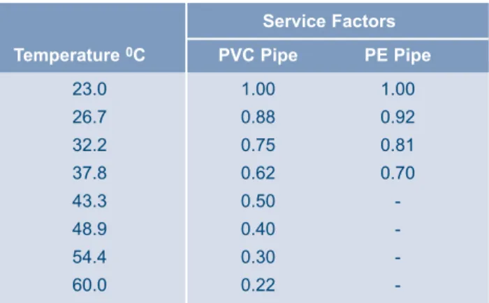
10.1. Effect of temperature 43
10.2. Effect of pipe material and the relationship between pipe diameter and wall thickness 43 10.3. Design and management considerations in dealing with water hammer 45
11. OPERATION AND MAINTENANCE OF PUMPING UNITS 47
11.1. Pump start-up and shut-down 47
11.1.1. Priming 47
11.1.2. Starting the pump 47
11.1.3. Stopping the pump 47
11.2. Pump malfunctions, causes and remedies (troubleshooting) 48
REFERENCES 49
Module 5 –v
List of figures
1. Sub-classification of pump types as a function of operating head and discharge 1 2. Schematic classification of pump types by the State Electricity Commission in 1965 2 3. Schematic classification of pump types by the Hydraulic Institute in 1983 34. Components of total dynamic head 5
5. Cross-section of a centrifugal pump 7
6. Pump impellers and volute casing 8
7. Classification of volute pumps based on impeller proportions 8
8. Parts of bowl assembly 9
9. Different drive configurations 10
10. Electrically driven turbine pump 11
11. Cross-section through a submersible pump and submersible motor 12
12. An example of a jet pump 13
13. Basic principles of positive displacement pumps 14
14. Hand pump with single acting bucket and piston 15
15. Double acting pressure treadle pump 16
16. Discharge-head relationship for pressure treadle pump (based on Table 1) 16
17. Double acting non-pressure treadle pump 17
18. Mono pump 18
19. Pump characteristic curves 19
20. Schematic presentation of Net Positive Suction Head Available (NPSHA) 21
21. TDH-Q curve for two pumps operating in series 22
22. TDH-Q curve for two pumps operating in parallel 22
23. Pump characteristic curves 25
24. Effect of speed change on centrifugal pump performance 26
25a. Performance curve of a pump 28
25b. Performance curve of a pump 29
26. Rating curves for engine 32
27. Foundation of a pumping unit and the reinforcement requirements 38
List of tables
1. Pressure treadle pump test analysis 15
2. Variation of vapour pressure with temperature 20
3. Comparison of the energy requirements for the three irrigation systems for different static lifts 36
4. Temperature service rating factors for PVC and PE pipes 43
5. Recommended maximum surge heads for PVC pipes of different classes 43
6. Pump problems, causes and corrections 48
List of abbreviations
AC Asbestos Cement
ASAE American Society of Agricultural Engineers
BP Brake Power
d inside pipe diameter e vapour pressure of water
E Efficiency
E Elasticity of pipe material
EFF Efficiency
fps feet per second g gravitational force
g gallon
H Head
HP Horse Power
Kpa Kilopascal
kW kilowatt
L Length
N Speed
NPSHA Net Positive Suction Head Available NPSHR Net Positive Suction Head Required
P Pressure
PE Polyethylen
PVC Polyvinyl Chloride
Q Discharge
rpm revolutions per minute SEC State Electricity Commission t pipe wall thickness
T Time
TDH Total Dynamic Head
uPVC unplasticized Polyvinyl Chloride
V Velocity
WP Water Power
Z Elevation
ZITC Zimbabwe Irrigation Technology Centre
Most irrigation pumps fall within the category of pumps that use kinetic principles, that is centrifugal force or momentum, in transferring energy. This category includes pumps such as centrifugal pumps, vertical turbine pumps, submersible pumps and jet pumps. Most of these pumps operate within a range of discharge and head where the discharge will vary as the head fluctuates.
The second category of pumps is that of positive displacement pumps, whereby the fluid is displaced by mechanical devices such as pistons, plungers and screws. Mono pumps, treadle pumps and most of the manual pumps fall into this category.
Allahwerdi (1986) calls the first category of pumps turbo pumps and depending on the type of discharge subdivides these pumps into:
Y Radial flow pumps (centrifugal action) Y Axial flow pumps (propeller-type action) Y Mixed flow pumps (variation of both)
It should be noted that Allahwerdi's classification does not include positive displacement pumps.
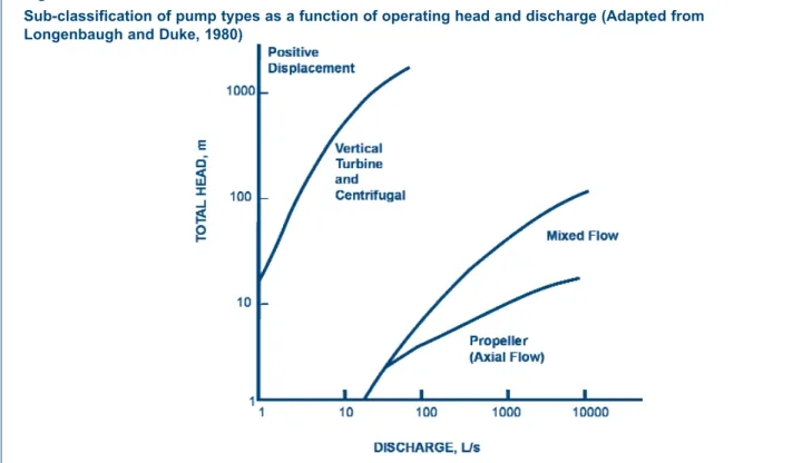
Longenbaugh and Duke (1980) classify pumps into:
Y Vertical turbine and centrifugal pumps Y Propeller or axial flow pumps
Y Mixed flow pumps
Y Positive displacement pumps
Figure 1 shows this classification as a function of the total operating head and discharge. The schematic classification employed by the State Electricity Commission (SEC) is shown in Figure 2 and the one employed by the Hydraulic Institute in Figure 3.
Positive displacement pumps are as a rule suitable for small discharges and high heads and the head is independent of the pump speed. Some types of these pumps should only be used with water free of sediments. The vertical turbine and the centrifugal pumps fit conditions of moderately small to high discharges and moderately low to high heads. These are the most commonly used pumps in irrigation. They can operate with reasonable amounts of sediments, but periodic replacement of impellers and volute casing should
Module 5 –1
Chapter 1
Introduction
Figure 1
Sub-classification of pump types as a function of operating head and discharge (Adapted from Longenbaugh and Duke, 1980)
be anticipated. Turbine pumps are more susceptible to sediments than centrifugal pumps. Mixed flow pumps cover a good range, from moderately large to large
discharges, and moderately high heads. They have the same susceptibility to sediments as do centrifugal pumps. Axial flow pumps are suitable for low heads and large discharges.
2 – Module 5
Figure 2
Module 5 –3
Module 5: Irrigation pumping plant
Figure 3
Head is the expression of the potential energy imparted to a liquid to move it from one level to another. Total dynamic head or total pumping head is the head that the pump is required to impart to a fluid in order to meet the head requirement of a particular system, whether this be a town water supply system or an irrigation system. The total dynamic head is made up of static suction lift or static suction head, static discharge head, total static head, required pressure head, friction head and velocity head. Figure 4 shows the various components making up the total dynamic head.
2.1. Static suction head or static suction lift
When a pump is installed such that the level of the water source is above the eye of the impeller (flooded suction), then the system is said to have a positive suction head at the eye of the impeller. However, when the pump is installed above the water source, the vertical distance from the surface of the water to the eye of the impeller is called the static suction lift.
2.2. Static discharge head
This is the vertical distance or difference in elevation between the point at which water leaves the impeller and the point at which water leaves the system, for example the outlet of the highest sprinkler in an overhead irrigation system.
2.3. Total static head
When no water is flowing (static conditions), the head required to move a drop of water from a (water source) to b (the highest sprinkler or outlet point) is equal to the total static head. This is simply the difference in elevation between where we want the water and where it is now. For systems with the water level above the pump, the total static head is the difference between the elevations of the water and the sprinkler (Figure 4a).
Total Static Head = Static Discharge Head – Static Suction Head
For systems where the water level is below the pump, the
Module 5 –5
Chapter 2
Total dynamic head or total pumping head
Figure 4
total static head is the static discharge head plus the static suction lift (Figure 4b).
Total Static Head = Static Discharge Head + Static Suction Lift
2.4. Friction head
When water flows through a pipe, the pressure decreases because of the friction against the walls of the pipe. Therefore, the pump needs to provide the necessary energy to the water to overcome the friction losses. The losses must be considered both for the suction part and the discharge part of the pump. The magnitude of the friction head can be calculated using either hydraulic formulae or tables and graphs.
2.5. Pressure head
Except for the cases where water is discharged to a reservoir, or a canal, a certain head to operate an irrigation system is required. For example, in order for a sprinkler system to operate, a certain head is required.
2.6. Velocity head
This energy component is not shown in Figure 4. It is very small and is normally not included in practical pressure calculations. Most of the energy that a pump adds to flowing water is converted to pressure in the water. Some of the energy is added to the water to give the velocity it requires to move through the pipeline. The faster the water is moving the larger the velocity head. The amount of energy that is needed to move water with a certain velocity is given by the formula:
Equation 1
Velocity Head = V2 2g Where:
V = the velocity of the water (m/s)
g = the gravitational force which is equal to 9.81 (m/s2)
Keller and Bliesner (1990) recommend that for centrifugal pumps the diameter of the suction pipe should be selected such that the water velocity V < 3.3 m/s in order to assure good pump performance. Assuming this maximum velocity for the flow and applying the above formula, then the velocity head corresponding to the minimum diameter of the suction pipe that can be selected to satisfy this condition is 0.56 m/sec (3.32/(2 x 9.81)).
2.7. Drawdown
Usually, the level of the water in a well or even a reservoir behind a dam does not remain constant. In the case of a well, after pumping starts with a certain discharge, the water level lowers. This lowering of the water level is called drawdown. In the case of a dam or reservoir, fluctuation of the water level is common and depends on water inflow, evaporation and water withdrawal. The water level increases during the rainy season, followed by a decrease during the dry season because of evaporation and withdrawal of the stored water. This variation in water level will affect the static suction lift or the static suction head and, correspondingly, the total static head.
3.1. Radial flow pumps
Radial flow pumps are based on the principles of centrifugal force and are subdivided into volute pumps and diffuser (turbine) pumps.
3.1.1 Volute pumps
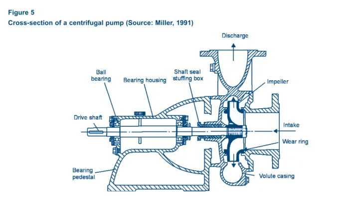
The well-known horizontal centrifugal pump is a volute pump. The pump consists of two main parts, the propeller that rotates on a shaft and gives the water a spiral motion, and the pump casing that directs the water to the impeller through the volute and eventually to the outlet. The suction entrance of the casing is in such a position that the water enters the eye of the impeller. The water is then pushed outwards because of the centrifugal force caused by the rotating impeller. The centrifugal force, converted to velocity head and thus pressure, pushes the water to the outlet of the volute casing. Figure 5 shows the components of a typical centrifugal pump.
Figure 6 shows the impeller inside the volute casing and the three types of impellers commonly used in centrifugal pumps. Closed impellers develop higher efficiencies in
high-pressure pumps. The other two types are more able to pass solids that may be present in the water.
Volute pumps may be classified under three major categories (Figure 7):
Y Low head, where the impeller eye diameter is relatively
large compared with the impeller rim diameter
Y Medium head, where the impeller eye diameter is a
small proportion of the impeller rim diameter
Y High head, where the impeller rim diameter is
relatively much larger than the impeller eye diameter
3.1.2. Diffuser or turbine pumps
The major difference between the volute centrifugal pumps and the turbine pumps is the device used to receive the water after it leaves the impeller.
In the case of the turbine pumps, the receiving devices are diffuser vanes that surround the impeller and provide diverging passages to direct the water and change the velocity energy to pressure energy. Deep well turbine pumps and submersible pumps use this principle.
Module 5 –7
Chapter 3
Types of pumps and principles of operation
Figure 5
8 – Module 5
Figure 6
Pump impellers and volute casing (Source: T-Tape, 1994)
Figure 7
Module 5 –9
Module 5: Irrigation pumping plant
Figure 8
10 – Module 5
Figure 9
Module 5 –11
Module 5: Irrigation pumping plant
Figure 10
Depending on the required head, these pumps have a number of impellers, each of which is enclosed with its diffuser vanes in a bowl. Several bowls form the bowl assembly that must always be submerged in water. Figure 8 shows parts of the bowl assembly. A vertical shaft rotates the impellers. In the case of turbine pumps the shaft is located in the centre of the discharge pipe. At intervals of usually 2-3 m, the shaft is supported by rubber lined water lubricated bearings. Figure 9 shows different drive configurations. Figure 10 shows a complete electrically driven turbine pump.
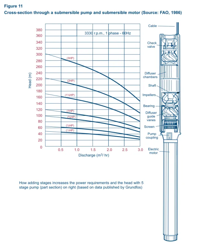
Electro-submersible pumps are turbine pumps with an electric motor attached in the suction part of the pump, providing the drive to the shaft that rotates the impellers. Therefore, there is no shaft in the discharge pipe. Both the motor and pump are submerged in the water. They are especially suitable for installation in deep boreholes. Submersible electrically driven pumps depend on cooling via the water being pumped, and a failure of the water supply can result in serious damage to the unit. For this reason submersible pumps are protected with water level cut-off switches. Figure 11 shows a complete submersible pump.
12 – Module 5
Figure 11
Cross-section through a submersible pump and submersible motor (Source: FAO, 1986)
How adding stages increases the power requirements and the head with 5 stage pump (part section) on right (based on data published by Grundfos)
Module 5 –13
Module 5: Irrigation pumping plant
Figure 12
An example of a jet pump (Source: Grundfos, undated)
This deep well pumping system is deal for small water supply plants that are to take water from depths of more than 6/8 metres.
1. The ejector pump system is inexpensive to purchase initially and is quick and easy to install. 2. A separate pump house is not normally required
over the borehole/well, as the pump can be installed in the top of the well or in an existing adjacent building.
3. Electric cables are not needed in the well. 4. Comparatively low noise level – an even flow of
water.
5. Suitable tank pressure irrespective of depth. 6. Easy adjustment of pump output to match the well
capacity.
7. The pump is easily accessible for overhaul. 8. Sturdy and reliable even where there are long
horizontal pipe runs and great depths. Operation
The Grundfos ejector system consists of a vertical multistage centrifugal pump connected by two pipes to ejector (see illustration) which is situated below the water level in the well. The pump has a third connection, the discharge port and its position on the pump can be varied to give varying discharge pressure to suit the application.
The method of operation is as follows. The pump supplies water at high pressure down the pressure pipe B, through the strainer Eand into the nozzle D. In the nozzle the high pressure is converted into high velocity water jet which passes through the chamber into the diffusor C. The chamber is connected via the foot valve Gand the strainer Hto the well water. The water in the chamber Fis picked up by the high velocity water jet passing from the nozzle into the diffusor. Here the two water flows are mixed and the high velocity is converted into pressure, which forces the water up the riser pipe Ainto the pump suction chamber.
The use of a multistage centrifugal pump enables the discharge port to be positioned at a suitable stage to give the correct discharge pressure at maximum water output. This ensures optimum operating efficiency. At the same time the stages of the pump above the discharge port maintain the required pressure for the ejector, even when the discharge pressure falls too zero when the consumption is momentarily larger than the well capacity.
Grundfoshave developed this ejector system and the present range of pumps and ejectors have evolved from many years experienced under varying conditions ranging from the far North of Scandinavia to the far South of Australia.
The ejector body is made of bronze and fitted with a wear-resistant stainless steel nozzle, which is protected against blockage by the strainer E. The built-in foot valve has a cone of stainless steel, seating on rubber and the strainer is made of bronze.
The wide range of Grundfos centrifugal pumps, ejector pumps and submersible pumps are still being enlarged and improved and on the basis of extensive research are THE RIGHT PUMPSfor water supply.
3.2. Axial flow pumps
While the radial flow type of pump discharges the water at right angles to the axis of rotation, in the axial flow type water is propelled upwards and discharged nearly axially. The blades of the propeller are shaped somewhat like a ship's propeller. Axial flow type pumps are used for large discharges and low heads (see Figure 1).
3.3. Mixed flow pumps
This category includes pumps whereby the pressure head is developed partially through the centrifugal force and partially through the lift of the vanes on the water. The flow is discharged both axially and radially. These pumps are suitable for large discharges and medium head.
3.4. Jet pumps
This pump is a combination of a centrifugal pump and a nozzle converting high pressure into velocity (Figure 12). As such it cannot fit into one of the above categories. A high-pressure jet stream is ejected through a suitable nozzle to entrain a large volume of water at low pressure and force it to a higher level within the system. The pump has no moving parts in the well or beneath the water surface. It is composed of a multistage centrifugal pump installed above
ground, an ejector installed below the water surface and connecting pipes. The disadvantage of these units is that when they are used in high head situations, the discharge and efficiency are greatly reduced. Basically such units are categorized as:
Y Low head, large discharge – most efficient Y High head, low discharge – least efficient
3.5. Positive displacement pumps
3.5.1. Manual pumps
For all practical purposes, water is incompressible. Consequently, if a close-fitting piston is drawn through a pipe full of water it will displace water along the pipe (Figure 13). Similarly, raising a piston in a submerged pipe will draw water up behind it to fill the vacuum that is created, and water is actually displaced by atmospheric pressure on its external surface. Two examples of manual pumps employing these principles are described below.
Piston or bucket pumps
The most common and well-known form of displacement pump is the piston pump, also known as the bucket, hand or bush pump. A common example is
14 – Module 5
Figure 13
illustrated in Figure 14. Water is sucked into the cylinder through an inlet check valve or non-return valve on the upstroke, which is opened by the vacuum created. This vacuum also keeps the piston valve closed. On the down stroke, the check valve is held closed by both its weight and the water pressure. As this happens the piston valve is forced open as the trapped water is displaced through the piston ready for the next upstroke.
The piston valve has two leather cup washer seals. The outer casing and fittings are normally cast iron. While this pump is widely used in Zimbabwe for domestic water supplies, it is also used to irrigate gardens, but to a limited extent. These pumps have wide operating head ranges of 2 to 100 m depending on construction of the pump. Discharges of 15 to 25 m3/hr or 4 to 7 l/s could be
realized.
Treadle pumps
A treadle pump is another form of a positive displacement pump where the feet are used to treadle. Most treadle pumps are double acting, meaning that there is discharge on both the upstroke and downstroke. Figure 15 shows a typical double acting pressure treadle pump.
Tests carried out at the Zimbabwe Irrigation Technology Centre (ZITC) revealed that suction heads exceeding 3 m make the pump quite difficult to operate. In a similar argument, delivery heads in excess of 6 m are also not recommended. This shows that treadle pumps can only be used where there are shallow water tables. In semi arid regions, their use could be confined to vleis or dambos, where the water tables are shallow, or to draw water from dams or rivers.
Table 1 shows results of the tests carried out at ZITC on a pressure treadle pump. The data are plotted in Figure 16. Table 1
Pressure treadle pump test analysis
Total Dynamic Head (m) Discharge (= suction head + delivery head) (m3/hr)
3.5 6.9
5.0 4.9
6.0 3.7
Other models of treadle pump, based on the same principles but delivering water without pressure, have been used extensively in the Indian Sub-continent, as typified by
Module 5 –15
Module 5: Irrigation pumping plant
Figure 14
16 – Module 5
Figure 16
Discharge-head relationship for pressure treadle pump (based on Table 1) Figure 15
Double acting pressure treadle pump (Source: ZITC, 1997) Figure 17, and have recently been introduced in eastern and southern Africa. These types of treadle pump are also composed of two cylinders and two plungers. The pumped
water, instead of being delivered at the lower part of the pump through a valve box, is delivered at the top through a small channel. Figure 17 gives the details.
3.5.2. Motorized pumps Mono pumps
Mono pumps are motorized positive displacement pumps. Water is displaced by means of a screw type rotor that moves through the stator. As mono pumps fall in the positive displacement category the head is independent to the speed. However, the flow is about proportional to the speed. Figure 18 shows the individual components of a mono pump.
Module 5 –17
Module 5: Irrigation pumping plant
Figure 17
CHARACTERISTICS OF THE MONO BOREHOLE PUMP 1. SELF PRIMING. Due to the material used there is an
interference fit between Rotor and Stator. This close contact with the absence of valves or ports makes a very effective air exhauster as long as a lubricating film of water is present.
2. STEADY FLOW. Due to the line of seal which is a curve of constant shape moving through the stator at a constant axial velocity the rate of displacement is uniform and steady without any pulsation, churning or agitation.
3. POSITIVE DISPLACEMENT. As the Mono unit is a positive displacement pump the head developed is independent of the speed and the capacity approximately proportional to the speed.
4. SIMPLICITY. As the mono unity consists of a fixed stator with a single rotating element it is an extremely simple mechanism.
5. EFFICIENCY. Because of the continuous steady delivery coupled with the positive displacement the Mono pump has an extremely high efficiency.
6. COMPACTNESS. Although the Mono Pump is constructed on very robust lines the simplicity of its pumping principle and the absence of valves or gears makes a very compact and light weight unit.
7. ABRASION RESISTANCE. Due to the design of the stator and rotor, the position of the seal line is continuously changing both on the rotor and on the stator. This fact is the chief reason for the remarkable ability of the Mono Pump to handle water containing some sand. If, for instance, a piece of grit is momentarily trapped between the rotor and the stator, the resilient rubber stator yields to it without damage in the same way as a rubber tyre passes over a stone, and, owing to the instant separation of the two surfaces, the particle is at once released again and swept away by the water. There is no possibility of pieces of grit being embedded or dragged along between the two surfaces, which is the chief cause of the heavy wear of most other pumps when gritty water is being handled. The low velocity of the water through the pump and its steady continuous motion also contribute to freedom from wear.
8. VERSATILITY. The pump is suitable for electric motor or engine drive.
SPECIFICATIONS OF THE MONO BOREHOLE PUMP 1. Discharge head which also incorporates the pulley
housing consists of a cast iron body with gland from which the column is suspended. The pulley bearing assembly contains two pre-packed ball bearings, one being an angular contact thrust bearing.
2. Column piping is standard galvanized medium class water piping to British standard 1387/1967 with squared ends and B.S.P. thread.
3. Bobbin Bearing are styrene butadiene compound which grip the column pipe walls and support the drive shaft every 1.6m for the full length of the drive shaft. These bearings are water lubricated and the bearing piece of stainless steel.
4. Stabilizers are also a rubber compound stabilizing the column in the borehole every 13m.
5. The drive shafting is of high tensile carbon steel which allows for a minimum area usage in the pipe column but retains its strength as a positive drive.
6. The pump unit consists of a strainer, the element and the body.
7. The element is a stationary stator of a resilient neoprene based compound in the form of a compound internal helix vulcanised to the outer casing. A rotor with a hard chrome finish in the form of a single of double helix turns inside the stator. This maintains a full seal across the travelling constantly up the pump giving uniform positive displacement.
SCHEMATIC DIAGRAM OF UNIT
18 – Module 5
Figure 18
Module 5 –19 Most manufacturers provide four different characteristic
curves for every pump: the Total Dynamic Head versus Discharge or TDH-Q curve, the Efficiency versus Discharge or EFF-Q curve, the Brake Power versus Discharge or BP-Q curve and Net Positive Suction Head Required versus Discharge or NPSHR-Q curve. All four curves are discharge related. Figure 19 presents the four typical characteristic curves for a pump, with one stage or impeller.
4.1. Total dynamic head versus discharge (TDH-Q)
This is a curve that relates the head to the discharge of the pump. It shows that the same pump can provide different combinations of discharge and head. It is also noticeable that as the head increases the discharge decreases and vice versa.
Chapter 4
Pump characteristic curves
Figure 19
20 – Module 5
The point at which the discharge is zero and the head at maximum is called shut off head. This happens when a pump is operating with a closed valve outlet. As this may happen in the practice, knowledge of the shut off head (or pressure) of a particular pump would allow the engineer to provide for a pipe that can sustain the pressure at shut off point if necessary.
4.2. Efficiency versus discharge (EFF-Q)
This curve relates the pump efficiency to the discharge. The materials used for the construction and the finish of the impellers, the finish of the casting and the number and the type of bearings used affect the efficiency. As a rule larger pumps have higher efficiencies.
Efficiency is defined as the output work over the input work. Equation 2
E pump = Output work = WP = Q x TDH
Input work BP C x BP Where:
Epump = Pump efficiency
BP = Brake power (kW or HP = 1.34 x kW): energy imparted by the prime mover to the pump
WP = Water power (kW): energy imparted by the pump to the water
Q = Discharge (l/s or m3/hr)
TDH = Total Dynamic Head (m)
C = Coefficient to convert work to energy units – equals 102 if Q is measured in l/s and 360 if Q is measured in m3/hr
4.3. Brake or input power versus discharge (BP-Q)
This curve relates the input power required to drive the pump to the discharge. It is interesting to note that even at zero flow an input of energy is still required by the pump to operate against the shut-off head. The vertical scale of this curve is usually small and difficult to read accurately. Therefore, it is necessary that BP is calculated using Equation 3, which can be found by rearranging Equation 2:
Equation 3
BP = Q x TDH C x E pump
4.4. Net positive suction head required versus discharge (NPSHR-Q)
At sea level, atmospheric pressure is 100 kPa or 10.33 m of water. This means that if a pipe was to be installed vertically in a water source at sea level and a perfect vacuum created, the water would rise vertically in the pipe to a distance of 10.33 m. Since atmospheric pressure decreases with elevation, water would rise less than 10.33 m at higher altitudes.
A suction pipe acts in the manner of the pipe mentioned above and the pump creates the vacuum that causes water to rise in the suction pipe. Of the atmospheric pressure at water level, some is lost in the vertical distance to the eye of the impeller, some to frictional losses in the suction pipe and some to the velocity head. The total energy that is left at the eye of the impeller is termed the Net Positive Suction Head.
The amount of pressure (absolute) or energy required to move the water into the eye of the impeller is called the Net Positive Suction Head Requirement (NPSHR). It is a pump characteristic and a function of the pump speed, the shape of the impeller and the discharge. Manufacturers establish the NPSHR-Q curves for the different models after testing. If the energy available at the intake side is not sufficient to move the water to the eye of the impeller, the water will vaporize and the pump will cavitate (see Section 4.4.1). In order to avoid cavitation the NPSHA should be higher than the NPSHR required by the pump under consideration.
4.4.1. Cavitation
At sea level water boils at about 100°C and its vapour pressure is equal to 100 kPa. When water boils, air molecules dissolved in water are released back into air. The vapour pressure increases rapidly with temperature increase (Table 2) while atmospheric pressure decreases with altitude increase.
Table 2
Variation of vapour pressure with temperature (Source: Longenbaugh and Duke, 1980)
Temperature (°C) 0 5 10 15 20 25 30 35 40 45 50
Vapour pressure of 0.06 0.09 0.13 0.17 0.24 0.32 0.43 0.58 0.76 0.99 1.28
Figure 20
Schematic presentation of Net Positive Suction Head Available (NPSHA) (Source: T-Tape, 1994)
Module 5 –21
Module 5: Irrigation pumping plant
In the eye of the impeller of a pump, pressure may be reduced to such a point that the water will boil. As the water is carried to areas of higher pressure in the pump, the vapour bubbles will collapse or explode at the surface of the impeller blades or other parts of the pump, resulting in the material erosion. The phenomenon described here is known as cavitation. Cavitation makes itself noticeable by an increase in noise level (rattling sound), irregular flow, a drop in pump efficiency and sometimes in head. Heavy cavitation, especially in larger pumps, sounds like the roar of thunder. In order to determine the possibilities of the occurrence of cavitation, the water pressure at the pump's entrance is determined and compared with the vapour pressure at the temperature of the water to be pumped. For this purpose the NPSHA is calculated as follows:
Equation 4
NPSHA = atmospheric pressure at the given altitude – static suction lift – friction losses in pipe – vapour pressure of the liquids at the operating
temperature
Where:
– Atmospheric pressure at the given altitude, Pb = 10.33 – 0.00108 Z (Barometric
pressure)
Z = elevation (m) can be measured
– Static suction lift (m) can be measured
– Friction losses hl, in metres, can be calculated
from graphs and tables or formulae – Vapour pressure e (m) can be estimated
from Table 2
Gauge pressure (Figure 20) = static suction lift + friction losses in pipe + vapour pressure
If the NPSHA is less than the NPSHR, the NPSHA will have to be increased. This can be achieved by reducing the friction losses in the pipe by using a wider suction pipe, although this is not very effective. Generally, decreasing the static suction lift increases the NPSHA, which can be obtained by positioning the pump nearer to the water level (see Figure 4).
Example 1
Calculate the NPSHA for a pump to operate at an elevation of 2 000 m, under 35°C temperature. The friction losses in the suction pipe were calculated to be 0.7 m and the suction lift to be 2 m.
Pb = 10.33- 0.00108 x 2 000 = 8.17 m e = 0.58 m (from Table 2)
Therefore, using Equation 4:
22 – Module 5
4.5. Pumps in series
A good example of connecting pumps in series is where a centrifugal pump takes water from a dam and pumps it to another pump, which in turn boosts the pressure to the required level. Another example is the multistage turbine pump. In fact, each stage impeller represents a pump. In general, connecting pumps in series applies to the cases where the same discharge is required but more head is needed than that which one pump can produce.
For two pumps operating in series, the combined head equals the sum of the individual heads at a certain
discharge. Figure 21 shows how the combined TDH-Q curve can be derived. If pumps placed in series are to operate well, the discharge of these pumps must be the same.
The following equation from Longenbaugh and Duke (1980) allows the calculation of the combined efficiency at a particular discharge.
Equation 5
Eseries =
Q x (TDHa+ TDHb)
C x (BPa+ BPb)
Where:
E = Efficiency Q = Discharge (l/s)
TDH = Total Dynamic Head (m)
C = 102 (coefficient to convert work to energy units)
BP = Brake power (kW)
4.6. Pumps in parallel
Pumps are operated in parallel when, for roughly the same head, variation in discharge is required. A typical example would be a smallholder pressurized irrigation system with many users. In order to provide a certain degree of flexibility when a number of farmers cannot be present, due to other unforeseen obligations (for example funerals), several smaller pumps are used instead of one or two larger pumps. This has been practiced in a number of irrigation schemes in Zimbabwe. Figure 22 shows the TDH-Q combined curve, for two pumps in parallel.
Figure 21
TDH-Q curve for two pumps operating in series (Adapted from Longenbaugh and Duke, 1980)
Figure 22
Module 5 –23
Module 5: Irrigation pumping plant
The equation for the calculation of the combined efficiency is as follows:
Equation 6
Eseries =
(Qa+ Qb)) x TDH
C x (BPa+ BPb)
Where:
E = Efficiency Q = Discharge (l/s)
TDH = Total Dynamic Head (m)
C = 102 (coefficient to convert work to energy units)
BP = Brake power (kW)
It should be noted from this equation that each of the pumps used in parallel should deliver the same head and this has to be a criterion when selecting the pumps. At times, engineers are confronted with a situation where pumping is required from a number of different sources at different elevations. In this case each pump should deliver its water to a common reservoir and not a common pipe in order to avoid the flow of water from one pump to another.
Module 5 –25 In discussing pump characteristic curves, no mention of
speed was made. Figure 23, a typical manufacturer's characteristic curve, provides several TDH-Q, EFF-Q and BP-Q curves. This is because the same pump can operate at different speeds. A change in the impeller speed causes a shift of the Q-H characteristics in the diagram. It is a shift upwards and to the right with increasing speed and downwards and to the left when the speed is decreased. The BP required power also changes.
The relationship between speed, on the one hand, and discharge, head and power on the other is described by Euler's affinity laws in the Hydraulics Handbook of Colt Industries (1975) as follows (see also Figure 24):
Y The discharge Q varies in direct proportion to the speed: Equation 7
Q1
= N1 Q2 N2
Y The head H varies directly with the square of the speed: Equation 8
H1
= N1
2
H2 N2
Chapter 5
Speed variation
Figure 23
Example 2
If a pump delivers 40 l/s at a head of 32 m and runs at a speed of 1200 rpm, what would be the discharge and head at 2000 rpm? What would the brake power of the pump be if it were 16.78 kW at 1200 rpm?
Using Equation 7 the new discharge Q2would be:
Q1
= N1 40 1 200 Q2 = 40 x
2 000
= 66.7 l/s Q2 N2
⇒
Q2
=
2 000 ⇒ 1 200
Using Equation 8, the new head would be: H1
= N1
2 32 1 200 2
H2 = 32 x
2 000 2
= 88.9 m H2 N2
⇒
H2
=
2 000 ⇒ 1 200
BP2 is calculated using Equation 9 as follows:
BP1
= N1
3 16.78 1 200 3
⇒ BP2 = 16.78 x
2 000 3
= 77.7 kW BP2 N2
⇒
BP2
=
2 000 1 200
26 – Module 5
Figure 24
Effect of speed change on centrifugal pump performance (Adapted from Colt Industries, 1975) Y The break power BP varies approximately with the
cube of the speed: Equation 9
BP1
= N1
3
BP2 N2
Where:
Q1 = discharge and
H1 = head and
BP1 = brake power at N1speed in revolutions per
minute (rpm) Q2 = discharge and
H2 = head and
BP2 = brake power at N2speed in revolutions per
minute (rpm)
As a rule, most pump characteristic curves are presented with one speed only. Hence the need to use Euler's affinity laws in deriving performance at different speeds. Example 2 clarifies the process.
If the speed of the pump is changed from 1 200 rpm to 2 000 rpm, the discharge, head and brake power will change from 40 l/s to 66.7 l/s, 32 m to 88.9 m, and 16.8 to 77.7 kW respectively. However, the affinity laws make no reference as to how the pump efficiency is affected by speed changes. As a rule, pumps that are efficient at one speed would be efficient at other speeds.
Module 5 –27 The selection of pumps requires the use of manufacturers'
pump curves. As a first step, by looking at the various pump curves we can identify a pump that can provide the discharge and head required at the highest possible
efficiency. Following the identification of the pump, the NPHSR-Q curve is checked and evaluations are made to ensure that its NHPSA is higher than the NPHSR.
Chapter 6
Pump selection
Example 3
Let us assume that a designed sprinkler system would require a Q = 40 m3/hr at an H = 60 m. What would be the
best pump to select?
Looking at various performance curves provided by manufacturers (Figures 25a and 25b) the curve of Figure 25b was selected, as it appears to provide the highest efficiency (65%) for the required discharge and head requirements, compared to an efficiency of 45% given by curves of Figure 25a. Ideally we would have preferred a pump where the required head and flow combination falls on the right-hand side of the efficiency curve. With age, the operating point will move to the left, then we would be able to operate with higher efficiency. This pump should be equipped with the 209 mm impeller, as shown in the curve.
Looking at the NPSH-Q curve in Figure 25b, the NPSHR of this pump is 1.2 m. Assuming the following data for the site:
Y Elevation: 2 000 m Y Static suction: 2 m
Y Suction pipe friction losses: 0.5 m Y Maximum temperature: 35°C
Using Equation 4, NPSHA = (10.33 - 0.00108 x 2000) - 2.0 - 0.5 - 0.58 = 5.09 m
Since NPSHA (5.09 m) is higher than the NPSHR (1.2 m) of the selected pump no cavitation should be expected.
Example 4
Assuming a surface irrigation scheme requires a pump with a Q = 70 m3/hr delivered at an H = 23 m. In this case the
pump of Figure 25a would be more suitable. It can provide the required Q and H at an efficiency of 68%, using an impeller of 140 mm diameter.
If we opted to use a high pressure pump (Figure 25b) instead of a high volume low pressure pump (Figure 25a), the required Q of 70 m3/hr with 23 m head would fall outside the range of the pumps. Hence the efficiency would be very
28 – Module 5
Figure 25a
Module 5 –29
Module 5: Irrigation pumping plant
Figure 25b
30 – Module 5
When the required Q and H combination falls outside the performance curve or when it falls at the fringes of the performance curve, that type of pump should not be selected.
Another important consideration in selecting a pump is the size of the pump impeller. If the required Q and H combination falls between two impeller sizes, then the larger impeller will have to be used, but only after it is trimmed down by the manufacturers so that it matches the requested Q and H.
Module 5 –31 Most irrigation pumps are powered either with electric
motors or diesel engines. In some countries, natural gas, propane, butane and gasoline engines are also used to drive pumps. Wind and solar driven pumps are also used for pumping water, mostly for human and animal purposes. Chapter 4 described how to compute the size of the power unit. For centrifugal pumps and turbine pumps up to 20 m deep it is not necessary to compute the energy required to overcome bearing losses in the pump. For turbine pumps that are more than 20 m deep, the manufacturer's literature should be consulted on line shaft bearing losses.
7.1. Electric motors
For most centrifugal pumps the motors are directly coupled to the pump. This results in the elimination of belt drives and energy loss due to belt slippage, and safety hazards. Most centrifugal pumps used in Eastern and Southern Africa are coupled to the motor shaft through a flexible coupling.
In the past it was common practice to overload motors by 10-15% above the rated output without encountering problems. However, because of the materials currently used, motors can no longer stand this overloading. Therefore, they should be sized to the needed and projected future output.
For sustained use of a motor at more than 1 100 m altitude or at temperatures above 37°C derating may be necessary. Manufacturer's literature should be consulted for the
necessary derating. An example of the derating of diesel engines is shown in the following section.
7.2. Diesel engines
As a rule, petrol engines drive very small pumps. For most irrigation conditions, the diesel engine has gained popularity. It is more robust, requires less maintenance and has lower overall operation and maintenance costs. Most literature on engines uses English units of measurement. To convert kilowatts to horsepower a conversion factor of 1.34 can be applied. Horsepower versus speed curves (Figure 26) illustrate how output power increases with engine speed. However, there is a particular speed at which the engine efficiency is highest. This is the point at which the selected engine should operate. The continuous rated curve indicates the safest continuous duty at which the engine can be operated. Care should be taken to use the continuous rated output curve and not the intermittent output curve.
Manufacturer's curves are calculated for operating conditions at sea level and below 30°C. It is therefore necessary to derate the engines for different altitudes and temperatures where the operating conditions are different. According to Pair et al. (1983), derating is approximately 1% per 100 m increase in altitude and 1% per 5.6°C increase in air temperature from the published maximum output horsepower curve. On the top of that, an additional 5-10% for reserve should be deducted. If the continuous output curves are used, only the 5-10% deduction is applied.
Chapter 7
Power units
Example 5
What will be the output of a diesel engine with a speed of 2 600 rpm at 2 000 m altitude and a temperature of 35°C?
Referring to Figure 26, the maximum output at 2 600 rpm, by interpolation, would be around 114 hp, which falls outside the limits of this curve. By applying the above rule for 2 000 m altitude and 35°C, a deduction of 20% should be applied for elevation and 1% for temperature. An additional 10% should be applied for reserve. Therefore, the total deduction should be 114 x 0.31 = 35.3 HP, resulting in an output of 78.7 HP ( = 114 - 35.3).
If we apply the 10% deduction on the continuous rating curve then the output will be 80 - 8 = 72 HP. This is a more conservative approach.
Figure 26
Rating curves for engine (Source: Irrigation Association, 1983)
32 – Module 5
Tractors can also be used to drive pumps. However, it may not be an economically sound approach to permanently attach a tractor to a pump in view of the high capital cost of a tractor.
7.3. Power transmission
There are four types of transmission usually applied to irrigation pumps: direct coupling, flat belt, V-belt and gear. Direct coupling generally implies negligible or no loss of power. The loss of power through flat belt varies from 3-20%. Transmission losses for V-belt and gear drive, as a rule, do not exceed 5%.
Referring to our example, if we use direct coupling of engine to pump, the HP would remain 72 HP. If we use
gear or V-belt drive then the power available to the pump would be 68.4 HP (0.95 x 72). This should satisfy the input power requirements of the pump as calculated using Equation 3 and multiplying the result by 1.34 to convert to horsepower.
7.3.1. Overall derating
Most engineers multiply the result of Equation 2 by a factor of 1.2 and use the engine continuous output rating curve. In other words, they derate an engine by 20%.
Going back to the approaches described earlier in this chapter, the total derating on the continuous output curve is 10-15% for V-belt or gear (5-10% derating for continuous output and 5% for the transmission losses).
Module 5 –33 Energy requirements are proportional to the discharge,
head and efficiency of the pumping system as demonstrated by the formula used to calculate the kW power requirements (Equation 3):
BP = Q x TDH C x Epump
Where:
Q = discharge in l/s with C = 102 or in m3/hr with C = 360
TDH = Total Dynamic Head (m) Epump = pump efficiency
The annual or seasonal energy requirements increase with the increase of the total volume of water pumped annually or seasonally, and are therefore affected by the overall irrigation efficiency.
Motor efficiency also has a bearing on energy requirement calculations. According to Longenbaugh and Duke (1980), motor efficiencies are in the range of 0.88 - 0.92. Motors of 7.5 kW or less have motor efficiencies usually below 0.88. For motors of 75 kW or larger the efficiency is 0.9 -0.92. Hence, there is the tendency to use 0.88 for motor efficiency in small size irrigation schemes.
From the three examples below, localized irrigation would have the lowest energy requirements (2 741 kW/ha per year) followed by surface (3 743 kW/ha per year) and sprinkler (4 485 kW/ha per year), in that order. This is the result of higher irrigation efficiency combined with low operating pressure, in the case of drip irrigation. In the case of surface irrigation the lack of operating pressure puts it in the second place (before sprinkler) in terms of energy requirements, irrespectively of its low irrigation efficiency. The high operating pressure of the sprinkler system (30 m) makes this system the highest energy user.
Chapter 8
Energy requirements
Example 6
A 14 ha drag-hose sprinkler irrigation scheme, designed to satisfy 20 hours/day pumping at peak demand, requires a discharge of 57 m3/hr. Its TDH is 56 m (20 m static lift, 30 m sprinkler operating head and 6 m friction losses). The
net irrigation requirements are 131 250 m3/year. What are the energy requirements?
The total gross annual irrigation requirements at 75% irrigation efficiency are: 131 250
= 175 000 m3/ year
0.75
From the performance curves (Figure 25b) the best pump to satisfy this discharge and head has an efficiency of 0.69. Considering an overall derating of 20%, the power requirement is:
BP = 57 x 56 x 1.2 = 15.4 kW 360 x 0.69
Looking at the sizes commonly marketed (7.5 kW, 11 kW, 15 kW, 18 kW, 22kW, 30 kW, 40 kW, 55 kW, etc.), it appears that the 18 kW motor is the best choice for this scheme.
In order to pump the 175 000 m3annually the motor will be in operation for 3 070 hours (175 000/57). If the motor
efficiency is 0.88, the annual energy requirements would then be: 3 070 x 18
= 62 795 kW / year for 14 ha or 4 485 kWh/ha per year 0.88
34 – Module 5
Example 7
Assuming that the availability of water is not a constraint and that, instead of a sprinkler irrigation system, a surface irrigation system with 40% irrigation efficiency and a pumping lift of 25 m (assumed to be 20 m static lift plus 5 m friction losses), operating for 10 hours per day, is used. What would the energy requirements be?
Total gross annual irrigation water requirements: 131 250
= 328 125 m3/ year
0.4
Converting the discharge of 57 m3/hr for the drag-hose sprinkler system to a discharge for the surface irrigation
system gives a discharge of 213.5 m3/hr (57 x 20/10 x 0.75/0.4). Assuming the same efficiency of 69% for the best
pump to satisfy the discharge and TDH, the power requirements will be:
BP = 213.5 x 25 x 1.2 = 25.8 kW 360 x 0.69
From the standard sizes of motors available on the market, a 30 kW motor will be selected.
In order to pump the 328 125 m3of water annually the motor will have to operate for 1 537 hrs (328 125/213.5). The
energy requirements would then be: 1 537 x 30
= 52 398 kW / year for the 14 ha or 3 743 kWh/ha per year 0.88
Example 8
If, instead of a sprinkler or surface irrigation system, a localized irrigation system with 90% irrigation efficiency and a pumping lift of 40 m (static lift of 20 m, friction losses and operating head assumed to be 20 m), operating for 20 hours per day, is used. What would the energy requirements be?
Total gross annual irrigation water requirements: 131 250
= 145 833 m3/ year
0.9
Converting the discharge of 57 m3/hr for the drag-hose sprinkler system to a discharge for the localized irrigation
system gives a discharge of 47.5 m3/hr (57 x 20/20 x 0.75/0.9). Again assuming a pump efficiency of 69%, the power
requirements would be:
BP = 47.5 x 40 x 1.2 = 9.2 kW 360 x 0.69
Although a 9.2 kW motor is required, from the standard size motors available on the market an 11 kW motor will be selected.
In order to pump the 145 833 m3of water annually the motor will have to operate for 3 070 hrs (145 833/47.5). The
total annual irrigation energy requirements would then be: 3 070 x 11
= 38 375 kW / year for the 14 ha or 2 741 kWh/ha per year 0.88
Module 5 –35
Module 5: Irrigation pumping plant
In Example 9 surface irrigation is the most energy inefficient, because of the combined low irrigation efficiency and high static head. Localized irrigation again has lowest demand or highest efficiency.
Table 3 presents a comparison of energy requirements for sprinkler, surface and localized irrigation systems for different static lifts and operating pressures.
Following the same procedures described in Examples 6, 7, 8 and 9, the comparison of energy requirements of Table 3 was prepared. This comparison is based on net annual water requirements of 9 375 m3/ha per year and
an efficiency of 75% for sprinklers, 40% for surface and 90% for localized irrigation. The total area is assumed to be 14 ha. The flow rate used for sprinklers is 57 m3/hr,
for surface irrigation 213.5 m3/hr and for localized 47.5
m3/hr. For all systems a pump efficiency of 69% and a
motor efficiency of 88% were assumed. It should be noted that no adjustment of the kW requirements was made to match the availability of motors in the market, because the sizes of motors available vary from country to country.
For surface irrigation, the head losses for conveying the water to the night storage reservoir were assumed to be 5 m. In the case of sprinkler irrigation, the sprinkler operating pressure was assumed to be 30 m and the head losses 6 m. For localized irrigation, the operating pressure plus the head losses were assumed to be 20 m. The picture changes when the static lift increases to 35 m, as demonstrated in Example 9.
Example 9
Assuming all figures of the previous three examples remain the same, except for the static lift, which increases from 20 m to 35 m. What would the energy requirements be?
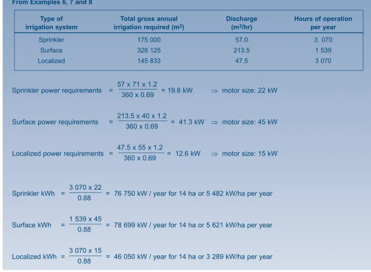
From Examples 6, 7 and 8
Type of Total gross annual Discharge Hours of operation irrigation system irrigation required (m3) (m3/hr) per year
Sprinkler 175 000 57.0 3 070
Surface 328 125 213.5 1 539
Localized 145 833 47.5 3 070
Sprinkler power requirements = 57 x 71 x 1.2 = 19.6 kW ⇒ motor size: 22 kW 360 x 0.69
Surface power requirements = 213.5 x 40 x 1.2 = 41.3 kW ⇒ motor size: 45 kW 360 x 0.69
Localized power requirements = 47.5 x 55 x 1.2360 x 0.69 = 12.6 kW ⇒ motor size: 15 kW
Sprinkler kWh = 3 070 x 22 = 76 750 kW / year for 14 ha or 5 482 kW/ha per year 0.88
Surface kWh = 1 539 x 45 = 78 699 kW / year for 14 ha or 5 621 kW/ha per year 0.88
Localized kWh = 3 070 x 15 = 46 050 kW / year for 14 ha or 3 289 kW/ha per year 0.88
36 – Module 5
The energy requirements comparison presented in Table 3 demonstrates the following:
Y The break-even point between sprinkler and surface
irrigation in terms of energy requirements occurs when both systems operate with a static lift of about 30 m.
Y As the static lift increases, the difference in the energy
requirements between surface and sprinkler irrigation increases substantially. The latter system requires less energy. This is attributed to the higher efficiency of sprinkler irrigation, which after the 30 m static lift point compensates for the higher pressure required by this system for its operation.
Y The break-even point between surface and localized
irrigation in terms of energy requirements falls somewhere between 5 and 10 m static lift (about 8 m). In this respect, it should be noted that low-pressure drip systems operating with 1-3 heads were not considered in this comparison.
Y As the static lift increases, the difference in energy
requirements between surface and localized systems increases, with the latter requiring less energy. This is attributed to the much higher efficiency of localized systems, which after the 8 m static lift point compensate for the higher pressure requirements of the localized systems.
Y Localized systems are less energy demanding than
sprinkler systems irrespective of static lift. This is attributed to the higher efficiency and lower operating pressure of the localized systems.
When electricity is not available and diesel engines are used for pumping, fuel requirements should be based on the manufacturer's catalogues as they vary according to the speed at which an engine operates. For example, a TS2 LISTER engine would consume 241 g/kWh at 1500 rpm or 266 g/kWh at 3000 rpm. As a rule a good estimate can be obtained by basing the diesel consumption on 0.25 litres/kWh.
Table 3
Comparison of the energy requirements for the three irrigation systems under different levels of static lift Power Annual Energy Requirements Annual Energy Requirements
Requirements for 14 ha per hectare
(kW) (kWh) (kWh/ha)
Static Surface Sprinkler Localized Surface Sprinkler Localized Surface Sprinkler Localized lift (m) irrigation irrigation irrigation irrigation irrigation irrigation irrigation irrigation irrigation
5 10.3 11.3 5.7 17 989 39 426 19 887 1 285 2 816 1 421
10 15.5 12.7 6.9 27 071 44 310 24 074 1 934 3 165 1 720
20 20.6 15.4 9.2 35 988 53 731 32 099 2 571 3 838 2 293
30 36.1 18.2 11.5 63 049 63 500 40 124 4 503 4 536 2 866
40 46.4 20.9 13.8 81 038 72 920 48 148 5 788 5 209 3 439
50 56.7 23.7 16.1 99 027 82 689 56 173 7 073 5 906 4 012
55 61.9 25.1 17.2 108 108 87 574 60 011 7 722 6 255 4 286
60 67.0 26.4 18.4 117 016 92 110 64 198 8 358 6 579 4 586
65 72.2 27.8 19.5 125 748 96 994 68 036 8 982 6 928 4 860
70 77.4 29.2 20.7 135 179 101 879 72 222 9 656 7 277 5 159
75 82.5 30.6 21.8 144 086 106 736 76 060 10 292 7 626 5 433
80 87.7 31.9 22.8 153 168 111 299 79 549 10 941 7 950 5 682
85 92.8 33.3 24.1 162 075 116 184 84 085 11 577 8 299 6 006
90 98.0 34.7 25.2 171 157 121 068 87 923 12 226 8 648 6 280
95 103.1 36.1 26.4 180 064 125 953 92 110 12 862 8 997 6 579
Module 5 –37
9.1. Siting of pumping station
The careful selection of a suitable location for a pumping station is very important in irrigation development. Several factors have to be taken into consideration when choosing the site.
Firstly, one has to find out whether the flow is reliable in the case of a river or whether the amount of water stored in the dam is enough to fulfil the annual irrigation requirements for the proposed cropping programme. This information is often obtained from the water authority or from the local farmers' experiences.
Secondly, in the case of river abstraction one has to check the maximum flood level of the river and preferably site the pumping station outside the flood level. With the limitations often imposed by the length of the suction pipe necessary to cater for the net positive suction head, where there are fluctuating flood levels, a portable pumping station is preferable. Such a site, however, should be on stable soil and have enough of water depth for the suction pipe. For permanent pumping stations pumps are installed on concrete plinth or foundation, the size of which varies in relation to the size of the pumping unit. Figure 27 shows a typical plinth and its reinforcement for pumps up to 50 kW. Thirdly, the abstraction point should not be sited in a river bend where sand and silt deposition may be predominant. Otherwise, the sand would clog both the suction pipe and pump. Where the river is heavily silted, a sand abstraction system can be developed.
Fourthly, where water is to be pumped from a dam or weir, the site should be outside the full supply level in case of upstream abstraction. In the case of downstream abstraction, the site should neither be too close to nor in line with the spillway.
Finally, as a rule, before a final decision is made on the location of the pumping station, a site visit has to take place to verify the acceptability of the site, taking into consideration the above requirements. It is generally helpful to talk to the local people to get information on the site. The cost of a pumping station will have to be divided into investment costs, costs of operation and costs of maintenance and repair. These costs will have to be
carefully estimated during the various stages of the design process in order to make comparisons for the different options more meaningful.
9.2. Installation of pump
When the correct type of pump has been selected it must be installed properly to give satisfactory service and be reasonably trouble-free. Pumps are usually installed with the shaft horizontal, occasionally with the shaft vertical (as in wells).
9.2.1. Coupling
Pumps are usually shipped already mounted, and it is usually unnecessary to remove either the pump or the driving unit from the base plate. The unit should be placed above the foundation and supported by short strips of steel plate and wedges. A spirit level should be used to ensure a perfect levelling. Levelling is a prerequisite for accurate alignment.
To check the alignment of the pump and drive shafts, place a straightedge across the top and side of the coupling, checking the faces of the coupling halves for parallelism. The clearance between the faces of the couplings should be such that they cannot touch, rub or exert a force on either the pump or the driver.
9.2.2. Grouting
The grouting process involves pouring a mixture of cement, sand and water into the voids of stone, brick, or concrete work, either to provide a solid bearing or to fasten anchor bolts. A wooden form is built around the outside of the bedplate to contain the grout and provide sufficient head for ensuring flow of mixture beneath the only bedplate. The grout should be allowed to set for 48 hours; then the hold-down bolts should be tightened and the coupling halves rechecked.
9.2.3. Suction pipe
The suction pipe should be flushed out with clear water before connection, to ensure that it is free of materials that might later clog the pump. The diameter of the suction pipe should not be smaller than the inlet opening of the
Chapter 9
Siting and installation of pumps
38 – Module 5
Figure 27
Module 5 –39
Module 5: Irrigation pumping plant
pump and it should be as short and direct as possible. If a long suction pipe cannot be avoided, then the diameter should be increased. Air pockets and high spots in a suction pipe cause trouble. After installation is completed, the suction pipe should be blanked off and tested hydrostatically for air leaks before the pump is operated. A strainer should be placed at the end of the inlet pipe to prevent clogging. Ideally the strainer should be at least four times as wide as the suction pipe. A foot valve may be installed for convenience in priming. The size of the foot valve should be such that frictional loses are very minimal.
9.2.4. Discharge pipe
Like the suction pipe, the discharge pipe should be as short and free of elbows as possible, in order to reduce friction. A gate valve followed by a check valve should be placed at the pump outlet. The non-return valve prevents backflow from damaging the pump when the pumping action is stopped. The gate valve is used to gradually open the water supply from the pump after starting and to avoid overloading the motor. The same valve is also used to shut off the water supply before switching off the motor.
Module 5 –41
Chapter 10
Water hammer phenomenon
Water hammer is the name given to the pressure surges caused by some relatively sudden changes in flow velocity. This can be caused by valve opening or closing, pump starting or stopping, cavitation or the collapse of air pockets in pipelines, filling empty pipelines or, of most concern to irrigation applications, a power outage, which suddenly shuts down all the electric pumps on the pipeline. When the velocity in the pipeline is suddenly reduced, the kinetic energy (velocity head) of the moving column of water is converted into potential energy (pressure head), compressing the water and stretching the pipewalls. These disturbances then travel up and down the pipeline as water hammer waves. The reader has probably experienced the banging and rattling of household pipework resulting from opening and closing a tap too rapidly – this is water hammer.
The pressure surges may either be positive or negative, i.e. the pressure may either rise above or fall below the operating pressure (static pressure, Po) by an amount equal to the maximum surge pressure, or surge head. The total pressure (Pt) rise due to water hammer is given by Joukowsky's Law (T-Tape, 1994), stated as:
Equation 10
Pt = Po + 0.07 x V x L T Where:
Pt = The total pressure developed in the system due to water hammer (psi)
Po = The static pressure (psi)
L = Length of pipe on the pressure side of the valve (feet) (3.28 feet = 1 m)
V = Velocity of water at the time the reduction occurred (fps) (3.28 fps = 1 m/s)
T = Valve closing time (s)
Another expression for the same purpose is provided through Equation 11. This equation takes the elasticity of the pipe material into consideration. It does not, however, take into account the valve time closure.
Equation 11
P = 1 423 x V x E
E + 294 000d t Where:
P = The excess pressure above normal (kPa) V = The velocity of flow (m/s)
E = Modulus of elasticity of the pipe material (for steel, cast iron, concrete and uPVC, E = 21 x 107, 0.5 x 10⁷, 2.1 x 10⁷and
0.28 x 10⁷respectively)
d = Pipe inside diameter (mm) t = Thickness of pipe wall (mm) 1423 = A constant for metric units
In Equation 11, V = V1-V2 where V1 is the upstream velocity and V2 is the downstream velocity of water in the pipe. As can be seen, the most severe case occurs when V2 becomes zero due to a sudden valve closure or similar action.
This equation calculates the surge pressure that would theoretically occur were the velocity instantaneously changed from V1 to V2. If a valve is closed slowly, the actual surge pressure will be less than this value. Thus, using this equation with V2 equal to zero (or V = V1) provides a safety factor.
Characteristics of the pipe, such as temperature, pipe material and the ratio of the diameter of the pipe to its wall thickness, affect the elastic properties of the pipe and will ultimately have an impact on the speed at which the shock waves travel up and down the pipe.
42 – Module 5
Example 10
An irrigation system has a uPVC mainline with a pressure rating of 125 psi. The velocity of flow is 5.29 fps. The system operating pressure (static) is 50 psi.
1. The longest length of uninterrupted piping between the source and valve is 100 feet and valve closure time is 10 seconds.
Pt = 50 + 0.07 x 5.29 x 100 = 50 + 3.7 = 53.7 psi 10
2. The longest length of uninterrupted piping between the source and valve is 100 feet and valve closure time is 1 second.
Pt = 50 + 0.07 x 5.29 x 100 = 50 + 37.0 = 87.0 psi 1
3. The longest length of uninterrupted piping between the source and valve is 1000 feet and valve closure time is 10 seconds.
Pt = 50 + 0.07 x 5.29 x 1000 = 50 + 37.0 = 87.0 psi 10
4. The longest length of uninterrupted piping between the source and valve is 1000 feet and valve closure time is 1 second.
Pt = 50 + 0.07 x 5.29 x 1000 1 = 50 + 370.3 = 420.3 psi. This is well above the pipe pressure rating of 125 psi
⇒ Severe water hammer damage
Example 11
The irrigation system in Example 10 has a uPVC mainline with a pressure rating of 125 psi. The velocity of flow is 5.29 fps. The system operating pressure (static) is 50 psi.
P = 1 423 x V x E E + 294 000d
t V = 5.29 fps = 1.61 m/s E = 0.28 x 10⁷for uPVC
d = 151.4 mm t = 4.59 mm
P = 1 423 x 1.61 x 0.28 x 10
7
0.28 x 10⁷+ 294 000 x151.4
4.59 P = 2291.03 x 0.47333
P = 1084.41 Kpa = 154.9 psi Pt = Po + P
Pt = 50 psi + 154.9 psi Pt = 204.9 psi