Data Structures for Strings
In this chapter, we consider data structures for storing strings; sequences of characters taken from some alphabet. Data structures for strings are an important part of any system that does text processing, whether it be a text-editor, word-processor, or Perl interpreter.
Formally, we study data structures for storing sequences of symbols over the alphabet Σ = {0, . . . ,|Σ|−1}. We assume that all strings are terminated with the special character $=|Σ|−1and that
$ only appears as the last character of any string. In real applications,Σmight be the ASCII alphabet
(|Σ|=128); extended ASCII or ANSI (|Σ|=256), or even Unicode (|Σ|=95, 221as of Version 3.2 of the
Unicode standard).
Storing strings of this kind is very dierent from storing other types of comparable data. On the one hand, we have the advantage that, because the characters are integers, we can use them as indices into arrays. On the other hand, because strings have variable length, comparison of two strings is not a constant time operations. In fact, the only a priori upper bound on the cost of comparing two strings
s1ands2isO(min(|s1|,|s2|}), where|s|denotes the length of the strings.
7.1 Two Basic Representations
In most programming languages, strings are built in as part of the language and they take one of two basic representations, both of which involve storing the characters of the string in an array. Both representations are illustrated in Figure 7.1.
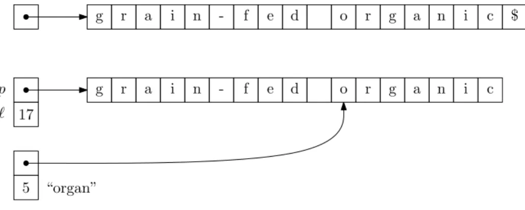
In the null-terminated representation, strings are represented as (a pointer to) an array of characters that ends with the special null terminator $. This representation is used, for example, in the C and C++ programming languages. This representation is fairly straightforward. Any character of the string can be accessed by its index in constant time. Computing the length,|s|, of a stringstakesO(|s|) time since we have to walk through the array, one character at a time until we nd the null terminator. Less common is the pointer/length representation in which a string is represented as (a pointer
o r g a n i c $ f e d
i n -g r a
o r g a n i c f e d
i n -g r a
17
5 “organ” p
`
Figure 7.1: The string \grain-fed organic" represented in both the null-terminated and the pointer/length representations. In the pointer/length representation we can extract the string \organ" in constant time. to) an array of characters along with a integer that stores the length of the string. The pointer/length representation is a little more exible and more ecient for some operations.
For example, in the pointer/length representation, determining the length of the string takes only constant time, since it is already stored. More importantly, it is possible to extract any substring in constant time: If a stringsis represented as(p, `)wherepis the starting location and`is the length,
then we can extract the substring si, si+1, . . . , si+m by creating the pair (p+i, m). For this reason several of the data structures in this chapter will use the pointer/length representation of strings.
7.2 Ropes
A common problem that occurs when developing, for example, a text editor is how to represent a very long string (text le) so that operations on the string (insertions, deletions, jumping to a particular point in the le) can be done eciently. In this section we describe a data structure for just such a problem. However, we begin by describing a data structure for storing a sequence of weights.
A prex tree T is a binary tree in which each nodevstores two additional values weight(v)and size(v). The value of weight(v)is a number that is assigned to a node when it is created and which may be modied later. The value of size(v)is the sum of all the weight values stored in the subtree rooted atv, i.e.,
size(v) = X u2T(v)
weight(u) .
It follows immediately that size(v)is equal to the sum of the sizes ofv's two children, i.e.,
size(v) =size(left(v)) +size(right(v)) . (7.1)
When we insert a new node u by making it a child of some node already in T, the only size
values that change are those on the path fromuto the root of T. Therefore, we can perform such an
insertion in time proportional to the depth of nodeu. Furthermore, because of identity (7.1), if all the
can maintain a prex-tree under insertions and deletions inO(logn)expected time per operation. Notice that, just as a binary search tree represents its elements in sorted order, a prex tree implicitly represents a sequence of weights that are the weights of nodes we encounter while travering
T using an in-order (left-to-right) traversal. Letu1, . . . , un be the nodes ofT in left-to-right order. We can use prex-trees to perform searches on the set
W=
wi:wi= i
X
j=1
weight(ui)
.
That is, we can nd the smallest value ofisuch thatwixfor any query valuex. To execute this kind of query we begin our search at the root ofT. When the search reaches some node u, there are three
cases
1. x <weight(left(u)). In this case, we continue the search forxin left(u).
2. weight(left(u))x <weight(left(u)) +weight(u). In this case, uis the node we are searching for,
so we report it.
3. weight(left(u)) +weight(u)x. In this case, we search for the value x0 =x−size(left(u)) −weight(u) in the subtree rooted at right(u).
Since each step of this search only takes constant time, the overall search time is proportional to the length of the path we follow. Therefore, if T is rebalanced as a treap then the expected search
time isO(logn).
Furthermore, we can support Split and Join operations in O(logn) time using prex trees. Given a valuex, we can split a prex tree into two trees, where one tree contains all nodesuisuch that
i
X
j=1
weight(ui)x
and the other tree contains all the remaining nodes. Given two prex trees T1 and T2 whose nodes in left-to-right order areu1, . . . , un andv1, . . . , vmwe can create a new treeT0whose nodes in left-to-right order areu1, . . . , un, v1, . . . , vn.
Next, consider how we could use a prex-tree to store a very long stringt=t1, . . . , tn so that it supports the following operations.
1. Insert(i, s). Insert the string s beginning at position ti in the string t, to form a new string
t1, . . . , ti−1sti+1, . . . , tn.1
2. Delete(i, l). Delete the substringti, . . . , ti+l−1fromSto form a new stringt1, . . . , ti−1, ti+l, . . . , tn. 1Here, and throughout,s
3. Report(i, l). Output the stringti, . . . , ti+l−1.
To implement these operations, we use a prex-tree in which each node u has an extra eld,
string(u). In this implementation, weight(u) is always equal to the length of string(u) and we can reconstruct the stringSby concatenating string(u1) string(u2) string(un). From this it follows that we can nd the character at positioni in Sby searching for the value i in the prex tree, which
will give us the nodeuthat contains the characterti.
To perform an insertion we rst create a new node v and set string(v) = s0. We then nd
the node u that contains ti and we split string(u) into two parts at ti; one part contains ti and the characters that occur before it and the second part contains the remaining characters (that occur after
ti). We reset string(u)so that it contains the rst part and create a new node wso that it string(w) contains the second part. Note that this split can be done in constant time if each string is represented using the pointer/length representation.
At this point the nodesv and w are not yet attached to T. To attach v, we nd the leftmost
descendant of right(u)and attachvas the left child of this node. We then update all nodes on the path
fromvto the root ofT and perform rotations to rebalanceT according to the treap rebalancing scheme.
Once v is inserted, we insert w in the same way, i.e., by nding the leftmost descendant of right(v). The cost of an insertion is clearly proportional to the length of the search paths forvandw, which are O(logn)in expectation.
To perform a deletion, we apply the Split operation on treaps to make three trees. The treeT1 containst1, . . . , ti−1, the treeT2containsti, . . . , ti+l−1and the treapT3that containsti+l, . . . , tn. This may require splitting the two substrings stored in nodes ofT that contain the indicesiand l, but the
details are straightforward. We then use the Merge operation of treaps to mergeT1andT3and discard
T2. Since Split and Merge in treaps each take O(logn) expected time, the entire delete operation takes inO(logn)expected time.
To report the string ti, . . . , ti+l−1 we rst search for the node u that contains ti and then traverseT starting at nodeu. We can then outputti, . . . , ti+l−1inO(l+logn)expected time by doing an in-order traversal ofT starting at nodeu. The details of this traversal and its analysis are left as an
exercise to the reader.
Theorem 18. Ropes support the operations Insert and Delete on a string of lengthninO(logn)
expected time and Report in O(l+logn)expected time.
7.3 Tries
Next, we consider the problem of storing a collection of strings so that we can quickly test if a query string is in the collection. The most obvious application of such a data structure is in a spell-checker.
A trie is a rooted tree T in which each node has somewhere between 0 and |Σ| children. All
edges ofT are assigned labels inΣsuch that all the edges leading to the children of a particular node
receive dierent labels. Strings are stored as root-to-leaf paths in the trie so that, if the null-terminated stringsis stored in T, then there is a leafv inT such that the sequence of edge labels encountered on
a o
r g
a n
s m
$ p
l e
$ $
e p
i $
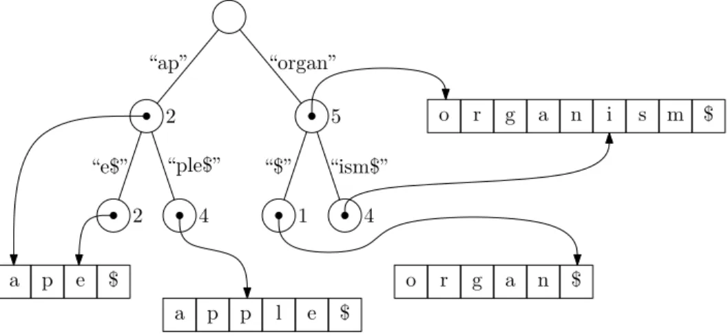
Figure 7.2: A trie containing the strings \ape", \apple", \organ", and \organism". shown in Figure 7.2.
Notice that it is important that the strings stored in a trie are null-terminated, so that no string is the prex of any other string. If this were not the case, it would be impossible to distinguish, for example, a trie that contained both \organism" and \organ" from a trie that contained just \organism". Implementation-wise, a trie node is represented as an array of pointers of size |Σ|, which point
to the children of the node. In this way, the labelling of edges is implicit, since theith element of the
array can represent the edge with label i−1. When we create a new node, we initialize all of its |Σ|
pointers to nil.
Searching for the stringsin a trie, T, is a simple operation. We examine each of the characters
ofsin turn and follow the appropriate pointers in the tree. If at any time we attempt to follow a pointer
that is nil we conclude thats is not stored inT. Otherwise we reach a leafv that representss and we
conclude thatsis stored inT. Since the edges at each vertex are stored in an array and the individual
characters ofsare integers, we can follow each pointer in constant time. Thus, the cost of searching for sisO(|s|).
Insertion into a trie is not any more dicult. We simply the follow the search path fors, and
“e$” “ple$” ‘$” “ism$” “ap” “organ”
Figure 7.3: A Patricia tree containing the strings \ape", \apple", \organ", and \organism". procedure runs inO(|s||Σ|)time.
Deletion from a trie is again very similar. We search for the leafv that representss. Once we
have found it, we delete all nodes on the path fromsto the root of T until we reach a node with more
than 1 child. This algorithm is easily seen to run inO(|s||Σ|)time.
If a trie holds a set ofnstrings,S, which have a total length ofNthen the total size of the trie
is O(N|Σ|). This follows from the fact that each character of each string results in the creation of at most 1 trie node.
Theorem 19. Tries support insertion or deletion of a string s in O(|s||Σ|) time and searching
fors inO(|s|) time. IfN is the total length of all strings stored in a trie then the storage used by
the trie is O(N|Σ|).
7.4 Patricia Trees
A Patricia tree (a.k.a. a compressed trie) is a simple variant on a trie in which any path whose interior vertices all have only one child is compressed into a single edge. For this to make sense, we now label the edges with strings, so that the string corresponding to a leafv is the concatenation of all the edge
labels we encounter on the path from the root ofT tov. An example is given in Figure 7.3.
The edge labels of a Patricia tree are represented using the pointer/length representation for strings. As with tries, and for the same reason, it is important that the strings stored in a patricia tree are null-terminated. Implementation-wise, it makes sense to store the edge label of an edgeuwdirected
from a parentuto it's childwin the node thew(since nodes can have many children, but at most one
parent). See Figure 7.4 for an example.
Searching for a string s in a Patricia tree is similar to searching in a trie, except that when
the search traverses an edge it checks the edge label against a whole substring of s, not just a single
character. If the substring matches, the edge is traversed. If there is a mismatch, the search fails without ndings. If the search uses up all the characters ofs, then it succeeds by reaching a leaf corresponding
tos. In any case, this takesO(|s|)time.
“ap”
a p e $
a p p l e $
o r g a n $
o r g a n i s m $ “organ”
“ism$” “ple$” “$”
“e$”
2 4 1 4
5 2
Figure 7.4: The edge labels of a Patricia tree use the pointer/length representation.
o r g a n i s m $ o r a n g e $
“orange$”
“or$”
“ganism$” “ange$”
“organism$”
Insert(“organism”) Delete(“orange”)
7 5 9
2
7
Figure 7.5: The evolution of a Patricia tree containing \orange$" as the string \organism$" is inserted and the string \orange$" is deleted.
actions of these algorithms. In this gure, a Patricia tree that initially stores only the string \orange" has the string \organism" added to it and then has the string \orange" deleted from it.
Inserting a stringsinto a Patricia tree is similar to searching right up until the point where the
search gets stuck becausesis not in the tree. If the search gets stuck in the middle of an edge,e, then e is split into two new edges joined by a new node,u, and the remainder of the string sbecomes the
edge label of the edge leading fromuto a newly created leaf. If the search gets stuck at a node,u, then
the remainder ofsis used as an edge label for a new edge leading fromuto a newly created leaf. Either
case takes O(|s|+|Σ|) time, since they each involve a search for sfollowed by the creation of at most
two new nodes, each of sizeO(|Σ|).
Removing a string s from a Patricia tree is the opposite of insertion. We rst locate the leaf
corresponding tosand remove it from the tree. If the parent,u, of this leaf is left with only one child, w, then we also remove uand replace it with a single edge, e, joining u's parent tow. The label for e
this takes depends on how long it takes to delete two nodes of size|Σ|. If we consider this deletion to be
a constant time operation, then running time isO(|s|). If we consider this deletion to takeO(N)time, then the running time isO(|s|+N).
An important dierence between Patricia trees and tries is that Patricia trees contain no nodes with only one child. Every node is either a leaf or has at least two children. This immediately implies that the number of internal (non-leaf) nodes does not exceed the number of leaves. Now, recall that each leaf corresponds to a string that is stored in the Patricia tree so if the Patricia tree storesnstrings, the
total storage used by nodes isO(n|Σ|). Of course, this requires that we also store the strings separately at a cost ofO(N). (As before,Nis the total length of all strings stored in the Patricia tree.)
Theorem 20. Patricia trees support insertion or deletion of any strings inO(|s|+|Σ|) time and
searching for s in O(|s|) time. If N is the total length of all strings and n is the number of all
strings stored in a Patricia tree then the storage used is O(n|Σ|+N).
In addition to the operations described in the preceding theorem, Patricia trees also support prex matches; they can return a list of all strings that have some not-null-terminated string s as a
prex. This is done by searching for s in the usual way until running out of characters ins. At this
point, every leaf in the subtree that the search ended at corresponds to a string that starts withs. Since
every internal node has at least two children, this subtree can be traversed inO(k)time, wherekis the
number of leaves in the subtree.
If we are only interested in reporting one string that hassas a prex, we can look at the edge
label of the last edge on the search path fors. This edge label is represented using the pointer/length
representation and the pointer points to a longer string that has s as a prex (consider, for example,
the edge labelled \ple$" in Figure 7.4, whose pointer points to the second `p' of \apple$"). This edge label can therefore be extended backwards to report the actual string that contains this label.
Theorem 21. For a query string s, a Patricia tree can report one string that has s as a prex
in O(|s|) time and can report all strings that have s as a prex in O(|s|+k) time, where k is the
number of strings that have s as a prex.
7.5 Suffix Trees
Suppose we have a large body of text and we would like a data structure that allows us to query if particular strings occur in the text. Given a stringtof lengthn, we can insert each of thensuxes of tinto a Patricia tree. We call the resulting tree the sux tree for t. Now, if we want to know if some
string soccurs in t we need only do a prex search for s in the Patricia tree. Thus, we can test if s
occurs int inO(|s|)time. In the same amount of time, we can locate some occurrence of sintand in O(|s|+k)time we can locate all occurrences ofsint, wherekis the number of occurrences.
What is the storage required by the sux tree forT? Since we only insertnsuxes, the storage
required by tree nodes is O(n|Σ|). Furthermore, recall that the labels on edges of T are represented
as pointers into the strings that were inserted intoT. However, every string that is inserted intoT is a
sux of t, so all labels can be represented as pointers into a single copy oft, so the total spaced used
to storetand all its edge labels is onlyO(n). Thus, the total storage used by a sux tree isO(n|Σ|). The cost of constructing the sux tree fort can be split into two parts: The cost of creating
of following paths, which is clearlyO(n ).
Theorem 22. The sux tree for a string t of length n can be constructed in O(n|Σ|+n2)time
and uses O(n|Σ|)storage. The sux tree can be used to determine if any string s is a substring
of t in O(|s|) time. The sux tree can also report the locations of all occurrences of s in t in O(m+k)time, where k is the number of occurrences of s in t.
The construction time in Theorem 22 is non-optimal. In particular, theO(n2)term is unnec-essary. In the next few section we will develop the tools needed to construct a sux tree inO(n|Σ|) time.
7.6 Suffix Arrays
The sux arrayA1, . . . , Anof a stringt=t1, . . . , tnlists the suxes oftin lexicographically increasing order. That is,Ai is the index such thattAi, . . . , tn has ranki among all suxes ofA.
For example, consider the stringt=\counterrevoluationary$":
1 2 3 4 5 6 7 8 9 10 11 12 13 14 15 16 17 18 19 20 21
c o u n t e r r e v o l u t i o n a r y $
The sux array fort isA=h18, 1, 6, 9, 15, 12, 17, 4, 11, 16, 2, 8, 7, 19, 5, 14, 3, 13, 10, 20, 21i. This is hard
to verify, so here is a table that helps:
i Ai tAi, . . . , tn
1 18 s1=\ary$"
2 1 s2=\counterrevolutionary$" 3 6 s3=\errevolutionary$" 4 9 s4=\evolutionary$" 5 15 s4=\ionary$" 6 12 s5=\lutionary$" 7 17 s7=\nary$"
8 4 s8=\nterrevolutionary$" 9 11 s9=\olutionary$" 10 16 s10=\onary$"
11 2 s11=\ounterrevolutionary$" 12 8 s12=\revolutionary$" 13 7 s13=\rrevolutionary$" 14 19 s14=\ry$"
15 5 s15=\terrevolutionary$" 16 14 s16=\tionary$"
17 3 s17=\unterrevolutionary$" 18 13 s18=\utionary$"
19 10 s19=\volutionary$" 20 20 s20=\y$"
Given a sux-array A = A1, . . . , An for t and a not-null-terminated query string s one can do binary search in O(|s|logn) time to determine whether s occurs in t; binary search uses O(logn) comparison and each comparison takesO(|s|)time.
7.6.1 Faster Searching with an` Matrix
We can do searches a little faster|inO(|s|+logn)time|if, in addition to the sux array, we have a little more information. Let si =tAi, tAi+1, . . . , tn. In other words, si is the string in theith row of
the preceding table. In other other words the string si is the ith sux of t when all suxes oft are sorted in lexicographic order.
Suppose, that we have access to a table`, where, for any pair of indices(i, j)with1ijn, `i,j is the length of the longest common prex ofsi and sj. In our running example,`9,11 = 1, since
s9=\olutionary$00 and s11=\ounterrevolutionary" have the rst character \o" in common but dier on their second character. Notice that this also implies that s10 starts with the same letter ass9 and
s11, otherwises10would not be betweens9ands11in sorted order. More generally, if`i,j =r, then the suxessi, si+1, . . . , sjall start with the samercharacters.
The value `i,j is called the longest common prex (LCP) of si and sj since it is the length of the longest string s0 that is a prex of both si and sj. With the extra LCP information provided by `, binary search on the sux array can be sped up. The sped-up binary search routine maintains
four integer valuesi, j,a and b. At all times, the search has deduced that a matching string|if it is
exists|is among si, si+1, . . . , sj (because si < s < sj) and that the longest prexes of si and sj that match shave lengtha andbrespectively. The algorithm starts with(i=1, j=n, a, b=0) where the value ofais obtained by comparingswith s1.
Suppose, without loss of generality, thatab(the case whereb > ais symmetric). Now,
con-sider the entry`i,m which tells us how many characters ofsm matchsi. As an example, suppose we are searching for the strings=\programmer", and we have reached a state wheresi=\programmable. . . $",
sj=\protectionism", soa=8 andb=3.:
si = \programmable. . . $" ...
sm = \pro. . . $" ...
sj = \protectionism. . . $"
Sincesiandsjshare the common prex \pro" of length min{a, b}=3, we are certain thatsmmust also have \pro" as a prex. There are now three cases to consider:
example of this occurs when sm=\progress. . . $", so that`i,m=5 and character at position 6 in
sm (an `e') is greater than the character at position 6 insi ands(an `a').
Therefore, our search can now be restricted tosi, . . . , sm. Furthermore, we know that the longest prex of sm that matchesshas lengthb0=`i,m. Therefore, we can recursively searchsi, . . . , sm using the valuesa0=aandb0=`i,m. That is, we recurse with the values(i, m, a, `i,m)
2. If `i,m > a, then we can immediately conclude that sm < s, for the same reason that si < s; namely si and s dier in character a+1 and this character is greater in s than it is in si and
sm. In this case, we recurse with the values (m, j, a, b). An example of this occurs when sm = \programmatically. . . $", so that `i,m = 9. In this case si and sm both have a `a' at position
a+1=9 whileshas an `e'.
3. If `i,m = a, then we can begin comparingsm ands starting at the(a+1)th character position. After matching k0 additional characters ofsandsm this will eventually result in one of three possible outcomes:
(a) Ifs < sm, then the search can recursive on the setsi, . . . sm using the values(i, m, a, a+k). An example of this occurs when sm = \programmes. . . $", so k = 1 and we recurse on (i, m, 8, 9).
(b) Ifs > sm, then the search can recurse on the setsm, . . . , sjusing the values(m, j, a+k, b). An example of this occurs whensm=\programmed. . . $", sok=1and we recurse on(m, j, 9, 3). (c) If all characters ofsmatch the rst|s|characters ofsm, thensm represents an occurrence of
sin the text. An example of this occurs whensm =\programmers. . . $".
The search can proceed in this manner, until the string is found at somesm or untilj=i+1. In the latter case, the algorithm concludes thatsdoes not occur as a substring oftsincesi< s < si+1.
To see that this search runs in O(|s|+logn)time, notice that each stage of the search reduces
j−i by roughly a factor of 2, so there are onlyO(logn)stages. Now, the time spent during a stage is proportional to k, the number of additional characters ofsm that match s. Observe that, at the end of the phase max{a, b}is increased by at leastk. Since aand bare indices into s,a|s|and b|s|.
Therefore, the total sum of all k values during all phases is at most |s|. Thus, the total time spent
searching forsisO(|s|+logn).
In case the search is successful, it is even possible to nd all occurences ofsin time proportional
to the number of occurrences. This is done by the nding the maximal integers x and y such that `m−x,m+y |s|. Finding x is easily done by trying x = 1, 2, 3, . . . until nding a value, x+1, such that `m−(x+1),m is less than |s|. Finding y is done in the same way. When this happens, all strings
sm−x, . . . , sm+yhave sas a prex.
Unfortunately, the assumption that we have an access to a longest common prex matrix`, is unrealistic and impractical, since this matrix has n
2
entries. Note, however, that we do not need to store`i,j for every valuei, j2{1, . . . , n}. For example, when nis one more than a power of 2, then we only need to know `i,j for values in which i = 1+q2p and j= i+2p, with p 2 {0, . . . ,blognc} and
q2{0, . . . ,bn/2pc}. This means that the longest common prex information stored in`consists of no more than
blogXnc i=0
values. In the next two sections we will show how the sux array and the longest common prex information can be computed eciently given the stringt.
7.6.2 Constructing the Suffix Array in Linear Time
Next, we show that a sux array can be constructed in linear time from the input string,t. The algorithm
we present makes use of the radix-sort algorithm, which allows us to sort an array ofnintegers whose
values are in the set{0, . . . , nc−1}inO(cn)time. In addition to being a sorting algorithm, we can also think of radix-sort as a compression algorithm. It can be used to convert a sequence, X, ofnintegers
in the range {0, . . . , nc−1}into a sequence, Y, ofn integers in the range{0, . . . , n−1}. The resulting sequence,Y, preserves the ordering ofX, so thatYi< Yjif and only ifXi< Xjfor alli, j2{1, . . . , n}.
The sux-array construction algorithm, which is called the skew algorithm is recursive. It takes as input a string s whose length is n, which is terminated with two $ characters, and whose
characters come from the alphabet{0, . . . n}.
Let S denote the set of all suxes of t, and let Sr, for r 2 {0, 1, 2} denote the set of suxes ti, ti+1, . . . , tnwhereir (mod3). That is, we partition the sets of suxes into three sets, each having roughlyn/3suxes in them. The outline of the algorithm is as follows:
1. Recursively sort the suxes inS1[S2. 2. Use radix-sort to sort the suxes in S0.
3. Merge the two sorted sets resulting from steps 1 and 2 to obtain the sorted order of the suxes in
S0[S1[S2=S.
If the overall running time of the algorithm is denoted byT(n), then the rst step takes T(2n/3)time and we will show, shortly, that steps 2 and 3 each take O(n)time. Thus, the total running time of the algorithm is given by the recurrence
T(n)cn+T(2n/3)cn
∞
X
i=0
(2/3)i3cn .
Next we describe how to implement each of the three steps eciently.
Step 1. Assumen=3k+1for some integerk. If not, then append at most two additional $ characters
to the end oftto make it so. To implement Step 1, we transform the stringtinto the sequence of triples: t0= (|t1, t2, t3),(t4, t5, t6){z, . . . ,(tn−3, tn−2, tn−1)}
suxes inS1
,|(t2, t3, t4),(t5, t6, t7){z, . . . ,(tn−2, tn−1, tn)}
suxes inS2
Observe that each sux in S1[S2 is represented somewhere in this sequence. That, is, for any
ti, ti+1, . . . , tn withi60 (mod3), the sux
will have sorted all the suxes in S1[S2. The string t0 contains about2n/3 characters, as required, but each character is a triple of characters in the range(1, . . . , n), so we cannot immediately recurse on
t0. Instead, we rst apply radix sort to relabel each triple with an integer in the range1, . . . , 2n/3. We
can now recursively sort the relabelled transformed string|which contains2n/3characters in the range 1, . . . , 2n/3|and undo the relabelling to obtain the sorted order of S1[S2. Aside from the recursive call, which takesT(2n/3)time, all of the sorting and relabelling takes onlyO(n)time.
When Step 1 is done, we know, for each indexi60 (mod3), the rank of the suxti, . . . , tnin the setS1[S2. This means that for any pair of indicesi, j60 (mod3), we can determine|in constant time, by comparing ranks|if the suxti, . . . , tn comes before or after the suxtj, . . . , tn.
Step 2. To implement Step 2, we observe that every sux in S0 starts with a single character and
is the followed by a sux in S1. That is, each sux ti, . . . , tn with i0 (mod3) can be represented as a pair (ti, `) where ` 2 {1, . . . , 2n/3) is the rank of the sux ti+1, . . . , tn obtained during Step 1. Applying radix sort to all of these pairs allows us to sortS0 inO(n)time.
Step 3. To implement Step 3, we have to merge two sorted lists, one of length2n/3and one of length
n/3inO(n)time. Merging two sorted lists usingO(n)comparisons is straightforward. Therefore, the only trick here is to ensure that we can compare two elements|one from the rst list and one from the second list|in constant time.
To see why this is possible, suppose we are comparingti, . . . , tn2S0withtj, . . . , tn 2S1. Then we can write these as comparing
ti, t|i+1, . . . , t{z n}
a sux inS1
and
tj, tj+1, . . . , tn
| {z }
a sux inS2 .
Now this can certainly be done in constant time, by comparingtiandtjand, in case of a tie, comparing two suxes whose relative order was already determined in Step 1.
Similarly, if we are comparing ti, . . . , tn 2 S0 with tj, . . . , tn 2 S2, then we can treat this as comparing
ti, ti+1, t|i+2, . . . , t{z n}
a sux inS2
and
tj, tj+1, tj+2, . . . , tn
| {z }
a sux inS1 .
This can also be done in constant time, by comparing at most two pairs of characters intand, if necessary
an sux in S1 with a sux inS2. The relative order of the suxes in S1 and S2 were determined in Step 1 of the algorithm.
1 2 3 4 5 6 7 8 9 10 11 12 13 14 15 16
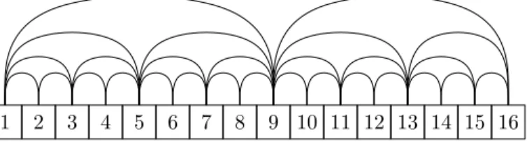
Figure 7.6: To implement binary search using a sux array, onlyO(n)LCP values are needed.
Theorem 23. Given a string t=t1, . . . , tn over the alphabet {1, . . . , n}, there exists an O(n)time
algorithm that can construct the sux array for t.
Of course, the preceding theorem can be generalized to larger alphabets. In particular, if the alphabet has sizenc, then the stringtcan be preprocessed inO(cn)time using radix sort to reduce the alphabet size ton. The sux array of the preprocessed string is then also a sux array for the original
string.
7.6.3 Constructing the Longest-Common-Prefix Array in Linear Time
As we have seen,O(|s|+logn)time searches in sux arrays make use of an auxiliary data structure to determine the length of the longest common prex between two suxessi andsj.
The longest common prex array (LCP array) of a sux array A=A1, . . . , An is an array
L = L1, . . . , Ln−1 where Li is the length of the longest common prex between si = tAi, . . . , tn and si+1=tAi+1, . . . , tn. That is,Lcontains information about lexicographically consecutive suxes of the
stringt. In terms of the notation in the previous section,Li=`i,i+1.
Before showing how to construct the LCP array, we recall that, in order to implement ecient prex searches in a sux array, we need more than an LCP array. Whennis a power of two, the binary
search algorithm needs to know the values`i,jfor all pairsi, jof formi=1+q2pandj=min{n, i+2p}, withp2{1, . . . ,dlogne−1}andq2{0, . . . ,dn/2pe}. See Figure 7.6 for an illustration.
To see that these can be eciently obtained from the longest common prex array, L, we rst
note that, for any1 i jn, `i,j = min{Li, Li+1, . . . , Lj−1}. Next, we observe that, the pairs(i, j)
needed by the binary search algorithm are nicely nested so that`i,j can be computed as the minimum of two smaller values. Specically,
`q2p,q2p+2p=min{`2q2p−1,2q2p−1+2p−1, `(2q+1)2p−1,(2q+1)2p−1+2p−1} .
(This is really easier to understand by looking at Figure 7.6 which shows that, for example,`9,13can be obtained as`9,13 = min{`9,11, `11,13}.) This allows for an easy algorithm that constructs the required values in a bottom up fashion, starting withp=1 (which is directly available from the LCP array,L)
and working up top=blognc. Each value can be computed in constant time and there are onlyO(n) values to compute, so converting the LCP array,Linto a structure useable for binary search can be done
inO(n)time. By doing this carefully, all the values needed to implement theO(|s|+logn)time search algorithm can be packed into a single array of length less than2n.
to do this uses an auxilliary array, R, which is the inverse of the sux array,A, so thatRAi =ifor all i2{1, . . . , n}. Another way to think of this is thatRigives the location ofAi. Yet another way to think of this is thatRi is the rank of the suxtAi, . . . , tn in the lexicographically sorted list of all suxes of t.
The algorithm processes the suxes in order of their occurrence in t. That is, t1, . . . , tn is processed rst. In our notation, this is suxsR1 and we want to compare it to the suxsR1−1in order
to determine the value of LR1−1. We can do this by comparing letter by letter to determine that the
length of the longest common prex ofsR1−1 andsR1 ish.
Things get more interesting when we move onto the string sR2 = t2, . . . , tn and we want to
compare it to sR2−1. Notice that the strings sR1 = t1, . . . , tn that we just considered and the string sR2=t2, . . . , tn that we are now considering have a lot in common. In particular, ifh > 0, then we can
be guaranteed thatsR2 matches the rsth−1characters ofsR2−1. Stop now and think about why this
is so, with the help of the following pictogram:
sR1=t1, t2 , t3 , . . . , th , . . .
= = = . . . = . . . sR1−1=ti, ti+1, ti+2, . . . , ti+h−1, . . .
= = . . . = . . . sR2= , t2 , t3 , . . . , th , . . .
The stringsR1−1is a proof thatthas some sux|namelyti+1, . . . , tn|that comes beforesR2
in sorted order and matches the rsth−1characters ofsR2. Therefore, the suxsR2−1that immediately
precedessR2 in sorted order must match at least the rsth−1 characters ofsR2. This means that the
comparison betweensR2 andsR2−1can start at thehth character position.
More generally, if the longest common prex of sRi andsRi−1 has length h, then the longest
common prex of SRi+1 and sRi+1−1 has length at least h−1. This gives the following very slick
algorithm for computing the LCP array,L.
BuildLCP(A, t) fori←1, . . . , ndo
RAi←i h←0
fori←1, . . . , ndo if Ri> 1then
k←ARi−1
whileti+h=tAk+h do
h←h+1 LRi−1←h h←max{h−1, 0}
returnL
The correctness of BuildLCP(A, t)follows from the preceding discussion. To bound the running time, we note that, with the exception of code inside the while loop, the algorithm clearly runs inO(n) time. To bound the total time spent in the while loop, we notice that the value ofhis initially 0, never
exceedsn, is incremented each time the body of the while loop executes, and is decremented at mostn
times. It follows that the body of the while loop can not execute more than2ntimes during the entire
execution of the algorithm.
Theorem 24. Given a sux array A for a string t of length n, the LCP array, L, can be
con-structed in O(n)time.
To summarize everything we know about sux arrays: Given a string t, the sux array,Afor tcan be constructed inO(n)time. FromAandt, the LCP array,L can be constructed inO(n)time. From the LCP array,L, an additional arrayL0of length2ncan be constructed that, in combination with Aandtmakes it possible to locate any stringsintinO(|s|+logn)time or report allkoccurrences of sint inO(|s|+logn+k)time..
In addition to storing the original text,t, this data structure needs the sux arrayA, of length nand the auxiliary arrayL0 of length2n. The values inAandL0 are integers in the range1, . . . , n, so
they can be represented using dlog2ne words. Thus, the entire structure for indexingtrequires only3n
words of space.
7.7 Linear Time Suffix Tree Construction
Although a sux array, in combination with an LCP array, is a viable substitute for a sux tree in many applications, there are still times when one wants a sux tree. In this section, we show that, given the sux array,A, and the LCP array,L, for the stringt, it is possible to compute the sux tree, T, fort inO(n|Σ|)time. Indeed, the tree structure can be constructed inO(n)time, the factor of|Σ|
comes only from creating an array of length|Σ|at each of the nodes in the sux tree.
The key observation in this algorithm is that the sux array and LCP array allow us to perform a traversal of the sux tree|creating nodes as we go. To see how this works, recall that the rst node traversed in an in-order traversal is lexicographically smallest. This node corresponds to the rst sux
s1 corresponding to the index, A1 in the sux array. We join this node, u1, to a sibling, u2 that corresponds tos2. The sibling leavesu1andu2are joined to a common parent,x, and the labels on the edgesxu1andxu2are suxes ofs1 ands2, respectively. The lengths of these labels can be computed by the length of the longest common prex betweens1ands2, which is given by the valueL1. And now we can continue this way using s3 and L2 to determine how the leaf, u3, corresponding tos3 ts into the picture. The length ofs2and the value ofL2 tells us whether
1. The parent ofu3should subdivide the edgexu2; or 2. The parent ofu3should bex; or
3. The parent ofu3should be a parent ofx.
In general, when we process the sux si, the length of si−1 and Li−1 are used to determine how the new leaf, ui should be attached to the partial tree constructed so far. Specically, these values allow the algorithm to walk upward fromui−1to nd an appropriate location to attachui. This will either result in
2. Attaching u3as the child of an existing node; or
3. A new parent foru3being created and becoming the root of the current tree.
Processingui may require walking up many, sayk, steps fromui−1, which takesO(k)time. However,
when this process walks past a node, this node is never visited again by the algorithm. Since the nal result is a sux tree that has at most 2n−1 nodes, the total running time is therefore O(n). The rst few steps of running this algorithm on the sux array for \counterrevolutionary$" are illustrated in Figure 7.7.
Theorem 25. Given a sux array and LCP array for a string t, the structure of the sux tree,
T, for t can be constructed in O(n) time. If one wants to also allocate and populate the arrays associated with the nodes of T then this can be done in an additional
7.8 Ternary Tries
The last three sections discussed data structures for storing strings where the running times of the operations were independent of the number of strings actually stored in the data structure. This is not to be underestimated. Consider that, if we store the collected works of Shakespeare in a sux tree, it is possible to test if the word \warble" appears anywhere in the text by following 7 pointers.
This result is possible because the individual characters of strings are used as indices into arrays. Unfortunately, this approach has two drawbacks: The rst is that it requires that the characters be integers. The second is that|Σ|, the size of the alphabet becomes a factor in the storage and running
time.
To avoid having|Σ|play a role in the running time, we can restrict ourselves to algorithms that
only perform comparisons between characters. One way to do this would be to simply store our strings in a binary search tree, in lexicographic order. Then a search for the stringscould be done withO(logn) string comparison, each of which takesO(|s|)time, for a total ofO(|s|logn).
Another way to reduce the dependence on|Σ| is to store child pointers in a binary search tree.
A ternary trie is a trie in which pointers to the children of each of nodevare stored in a binary search
tree. If we use a balanced binary search trees for this, then it is clear that the insertion, deletion and search times for the string sareO(|s|log|Σ|. IfN is large, we can do signicantly better than this, by
using a dierent method of balancing our search trees.
Note that a ternary trie can be viewed as a single tree in which each node has up to 3 children (hence the name). Each nodev has a left child, left(v), a right child, right(v), a middle child, mid(v), and is labelled with a character, denoted m(v). A root-to-leaf path Pin the tree corresponds to exactly
one string, which is obtained by concatenating the characters m(v)for each node vwhose successor in Pis a middle child.
Now, suppose that every node v of our ternary trie has the balance property |L(right(v))| |L(v)|/2 and |L(left(v))| |L(v)|/2, where L(v) denotes the set of leaves in the subtree rooted at v.
e v o l u t i o n
c o u n t e r r a r y $ 4
e v o l u t i o n
c o u n t e r r a r y $ 4 21
e v o l u t i o n
c o u n t e r r a r y $
4 21 16
e v o l u t i o n
c o u n t e r r a r y $ 4 21
1
15 12
Figure 7.7: Building a sux tree for \counterrevoluationary$" in a bottom-up fashion starting with the suxes \ary$", \counterrevoluationary$", \errevoluationary$", and \evoluationary$".
a mid pointer the number of symbols in s that are unmatched decreases by one and every time the
path traverses an edge represented by a left or right pointer the number of leaves in the current subtree decreases a factor of at least1/2.
Given a setS of strings, constructing a ternary trie with the above balance property is easily
done. We rst sort all our input strings and then look at the rst character,m, of the string whose rank
isn/2in the sorted order. We then create a new nodeuwith labelmto be the root of the ternary trie.
We collect all the strings that begin withm, strip o their rst character, and recursively insert these
into the middle child ofu. Finally, we recursively insert all strings beginning with characters less than uin the left child ofuand all strings beginning with characters greater thanuin the right child ofu.
Ignoring the cost of sorting and recursive calls, the above algorithm can easily be implemented to run inO(n0)time, wheren0is the number of strings beginning withm. However, during this operation,
we strip on0characters from strings and never have to look at these again. Therefore the total running
time, including recursive calls, is not more thanO(M), whereMis the total length of all strings stored
in the ternary trie.
Theorem 26. After sorting the input strings, a ternary trie can be constructed inO(M)time and
can search for a strings in O(|s|+logn) time.
TODO: Talk about how ternary quicksort can build a ternary search tree inO(M+nlogn). TODO: Talk about how to make ternary tries dynamic using treaps, splaying, weight-balancing, or partial rebuilding.
7.9 Quad-Trees
An interesting generalization of tries occurs when we want to store two (or more) dimensional data. Imagine that we want to store real values in the unit square[0, 1)2, where each point(x, y)is represented by two binary stringsx1, x2, x3, . . .andy1, y2, y3, . . .wherexi(respectivelyyi) is theith bit in the binary expansion ofx(respectively,y). When we consider the most-signicant bits of the binary expansion of xandy, four cases can occur:
(x, y) = (.0 . . . , .1 . . .) (.1 . . . , .1 . . .) (.0 . . . , .0 . . .) (.1 . . . , .0 . . .)
Thus, it is natural that we store our points in a tree where each node has up to four chil-dren. In fact, if we treat (x, y) as the string (x1, y1)(x2, y2)(x3, y3), . . . , over the alphabet Σ = {(0, 0),(0, 1),(1, 0),(1, 1)} and store (x, y) in a trie then this is exactly what happens. The tree that we obtain is called a quad tree.
Quad trees have many applications because they preserve spatial relationships very well, much in the way that tries preserve prex relationships between strings. As a simple example, we can consider queries of the form: report all points in the rectangle with bottom left corner [.0101010, .1111110]
and top right corner [.0101011, .1111111]. To answer such a query, we simply follow the path for (0, 1)(1, 1)(0, 1)(1, 1)(0, 1)(1, 1)in the quadtree (trie) and report all leaves of the subtree we nd.
Quadtrees can be generalized in many ways. Instead of considering binary expansions of thex
andycoordinates we can considerm-ary expansions, in which case we obtain a tree in which each node
has up tom2children. If, instead of points in the unit square, we have points in the unit hypercube in
Rdthen we obtain a tree in which each node has2dchildren. If we use a Patricia tree in place of a trie then we obtain a compressed quadtree which, like the Patricia tree uses onlyO(n+M)storage where
Mis the total size of (the binary expansion of) all points stored in the quadtree.
7.10 Discussion and References
Prex-trees seem be part of the computer science folklore, though they are not always implemented using treaps. The rst documented use of a prex-tree is unclear.
Ropes (sometimes called cords) are described by Boehm et al [3] as an alternative to strings represented as arrays. They are so useful that they have made it into the SGI implementation of the C++ Standard Template Library [?].
Tries, also known as digital search trees, have a very long history. Knuth [7] is a good resource to help unravel some of their history. Patricia trees were described and given their name by Morrison [10]. PATRICIA is an acronym for Practical Algorithm To Retrieve Information Coded In Alphanumeric.
Sux trees were introduced by Weiner [14], who also showed that, ifN, the size of the alphabet,
is constant then there is an O(n) time algorithm for their construction. Since then, several other simpliedO(n)time construction algorithms for sux trees have been presented [4, 8, 5].
Sux arrays were introduced by Manber and Myers [?], who gave anO(nlogn)time algorithm for their construction. TheO(n)time sux array construction algorithm given here is due to Karkainnen and Sanders [?], though several otherO(n)time construction algorithms are known [?]. The LCP array construction algorithm given here is due to Kasai et al [?].
Karwere viewed as an way of compressing sux trees [?]
Recently, Farach [5] gave an O(n) time algorithm for the case where N is as large as n, the
length of the string.
Ternary tries also have a long history, dating back at least until 1964, when Clampett [6] suggested storing the children of trie nodes in a binary search tree. Mehlhorn [9] shows that ternary tries can be rebalanced so that insertions and deletions can be done in O(|s|+logn) time. Sleator and Tarjan [12] showed that, if the splay heuristic (Section 6.1) is applied to ternary tries, then the cost of a sequence ofnoperations involving a set of strings whose total length is MisO(M+nlogn). Furthermore, with splaying, a sequence ofnsearches can be executed inO(M+nH)time, whereHis the
empirical entropy (Section 5.1) of the access sequence. Vaishnavi [13] and Bentley and Saxe [1] arrived at ternary tries through the geometric problem of storing a set of vectors in d-dimensions. Finally,
Bibliography
[1] J. L. Bentley and J. B. Saxe. Algorithms on vector sets. SIGACT News, 11(9):36{39, 1979. [2] J. L. Bentley and R. Sedgewick. Fast algorithms for sorting and searching strings. In Proceedings
of the Eighth Annual ACM-SIAM Symposium on Discrete Algorithms (SODA2000), pages 360{369, 1997.
[3] Hans-Juergen Boehm, Russ Atkinson, and Michael F. Plass. Ropes: An alternative to strings. Software|Practice and Experience, 25(12):1315{1330, 1995.
[4] M. T. Chen and J. Seiferas. Ecient and elegant subword tree construction. In A. Apostolico and Z. Galil, editors, Combinatorial Algorithms on Words, NATO ASI Series F: Computer and System Sciences, chapter 12, pages 97{107. NATO, 1985.
[5] M. Farach. Optimal sux tree construction with large alphabets. In 38th Annual Symposium on Foundations of Computer Science (FOCS'97, pages 137{143, 1997.
[6] H. H. Clampett Jr. Randomized binary searching with tree structures. Communications of the ACM, 7(3):163{165, 1964.
[7] Donald E. Knuth. The Art of Computer Programming. Volume III: Sorting and Searching. Addison-Wesley, 1973.
[8] E. M. McCreight. A space-economical sux tree construction algorithm. Journal of the ACM, 23(2):262{272, 1976.
[9] K. Mehlhorn. Dynamic binary searching. SIAM Journal on Computing, 8(2):175{198, 1979. [10] D. R. Morrison. PATRICIA - practical algorithm to retrieve information coded in alphanumeric.
Journal of the ACM, 15(4):514{534, October 1968.
[11] Hanan Samet. The Design and Analysis of Spatial Data Structures. Series in Computer Science. Addison-Wesley, Reading, Massachusetts, U.S.A., 1990.
[12] D. D. Sleator and R. E. Tarjan. Self-adjusting binary search trees. Journal of the ACM, 32(2):652{ 686, 1985.
[13] V. K. Vaishnavi. Multidimensional height-balanced trees. IEEE Transactions on Computers, C-33(4):334{343, 1984.
[14] P. Weiner. Linear pattern matching algorithm. In Proceedings of the 14th Annual IEEE Sym-posium on Switching and Automata Theory, pages 1{11, Washington, DC, 1973.