Computing and Rendering Point Set Surfaces

IEEE TVCG 9(1) Jan 2003

Computing and Rendering Point Set Surfaces

TU Darmstadt

Johannes Behr

ZGDV Darmstadt

Daniel Cohen-Or

Tel Aviv University

Shachar Fleishman

Tel Aviv University

David Levin

Tel Aviv University

Claudio T. Silva

AT&T Labs

Abstract

We advocate the use of point sets to represent shapes. We pro-vide a definition of a smooth manifold surface from a set of points close to the original surface. The definition is based on local maps from differential geometry, which are approximated by the method of moving least squares (MLS). The computation of points on the surface is local, which results in an out-of-core technique that can handle any point set.

We show that the approximation error is bounded and present tools to increase or decrease the density of the points, thus, allowing an adjustment of the spacing among the points to control the error.

To display the point set surface, we introduce a novel point ren-dering technique. The idea is to evaluate the local maps according to the image resolution. This results in high quality shading effects and smooth silhouettes at interactive frame rates.

CR Categories: I.3.3 [Computer Graphics]: Picture/Image Generation—Display algorithms; I.3.5 [Computer Graphics]: Computational Geometry and Object Modeling—Curve, surface, solid, and object representations;

Keywords: surface representation and reconstruction, moving least squares, point sample rendering, 3D acquisition

1

Introduction

Point sets are receiving a growing amount of attention as a repre-sentation of models in computer graphics. One reason for this is the emergence of affordable and accurate scanning devices generating a dense point set, which is an initial representation of the physical model [34]. Another reason is that highly detailed surfaces require a large number of small primitives, which contribute to less than a pixel when displayed, so that points become an effective display primitive [41, 46].

A point-based representation should be as small as possible while conveying the shape, in the sense that the point set is neither noisy nor redundant. In [1] we have presented tools to adjust the density of points so that a smooth surface can be well-reconstructed. Figure 1 shows a point set with varying density. Our approach is motivated by differential geometry and aims at minimizing the ge-ometric error of the approximation. This is done by locally approx-imating the surface with polynomials using moving least squares (MLS). Here, we include proofs and explanations of the

underly-Figure 1: A point set representing a statue of an angel. The density of points and, thus, the accuracy of the shape representation are changing (intentionally) along the vertical direction.

ing mathematics, detail a more robust way to compute points on the surface, and derive bounds on the approximation error.

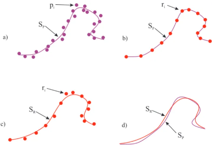
We understand the generation of points on the surface of a shape as a sampling process. The number of points is adjusted by either up-sampling or down-sampling the representation. Given a data set of points P={p_i}(possibly acquired by a 3D scanning device), we define a smooth surface S_P (MLS surface) based on the input points (the definition of the surface is given in Section 3). We sug-gest replacing the points P defining S_Pwith a reduced set R={r_i} defining an MLS surface S_Rwhich approximates S_P. This general paradigm is illustrated in 2D in Figure 2: Points P, depicted in pur-ple, define a curve S_P(also in purple). S_Pis re-sampled with points r_i∈S_P(red points). This typically lighter point set called the repre-sentation points now defines the red curve S_Rwhich approximates

a)

d) c)

b)

pi ri

SP

SR SR

ri

SP

SP

Figure 2: An illustration of the paradigm: The possibly noisy or re-dundant point set (purple points) defines a manifold (purple curve). This manifold is sampled with (red) representation points. The rep-resentation points define a different manifold (red curve). The spac-ing of representation points depends on the desired accuracy of the approximation.

S_P.

Compared to the earlier version [1] we give more and new details on the (computational) properties of the surface definition:

Smooth manifold: The surface defined by the point set is a

2-manifold and expected to be C∞smooth, given that the points are sufficiently close to the smooth surface being represented.

Bounded sampling error: Let S_Rbe defined by the set of repre-sentation points{r_i} ⊂S_P. The representation has bounded errorε, if d(S_P,S_R)<ε, where d(·,·)is the Hausdorff dis-tance.

Local computation: For computing a point on the surface only a

local neighborhood of that point is required. This results in a small memory footprint, which depends only on the antici-pated feature size and not the number of points (in contrast to several other implicit surface definitions, e.g. those based on radial basis functions).

In addition to giving more implementation details for the ren-dering method from [1], we give a justification that builds on the error bounds introduced here. This connection to the bounded error substantiates the claimed properties of our rendering scheme:

High quality: Since S_R is a smooth surface, proper re-sampling leads to smooth silhouettes and normals resulting in superior rendering quality at interactive frame rates.

Single step procedure: Re-sampling respects screen space

resolu-tion and guarantees sufficient sampling, i.e. no holes have to be filled in a post-processing step.

2

Related work

Consolidation

Recent technological and algorithmic advances have improved the process of automatic acquisition of 3D models. Acquiring the ge-ometry of an object starts with data acquisition, usually performed with a range scanner. This raw data contains errors (e.g., line-of-sight error [21, 47]) mainly due to noise intrinsic to the sensor used

and its interaction with the real-world object being acquired. For a non-trivial object, it is necessary to perform multiple scans, each in its own coordinate system, and to register the scans [6]. In gen-eral, areas of the objects are likely to be covered by several samples from scans performed from different positions. One can think of the output of the registration as a thick point set.

A common approach is to generate a triangulated surface model over the thick point set. There are several efficient triangulation techniques, such as [2, 3, 5, 7, 17]. One of the shortcomings of this approach is that the triangulated model is likely to be rough, con-taining bumps and other kinds of undesirable features, such as holes and tunnels, and be non-manifold. Further processing of the trian-gulated models, such as smoothing [51, 14] or manifold conver-sion [20], becomes necessary. The prominent difficulty is that the point set might not actually interpolate a smooth surface. We call consolidation the process of “massaging” the point set into a sur-face. Some techniques, such as Hoppe et al [23], Curless and Levoy [12], and Wheeler et al [55] consolidate their sampled data by us-ing an implicit representation based on a distance function defined on a volumetric grid. In [23], the distances are taken as the signed distance to a locally defined tangent plan. This technique needs further processing [24, 22] to generate a smooth surface. Curless and Levoy [12] use the structure of the range scans and essentially scan convert each range surface into the volume, properly weight-ing the multiply scanned areas. Their technique is robust to noise and is able to take relative confidence of the samples into account. The work of Wheeler et al [55] computes the signed distance to a consensus surface defined by weighted averaging of the different scans. One of the nice properties of the volumetric approach is that it is possible to prove under certain conditions that the output is a least-square fit of the input points (see [12]).

The volumetric sign-distance techniques described above are re-lated to a new field in computer graphics called Volume Graphics pioneered by Kaufman and colleagues [26, 54, 50] which aims to accurately define how to deal with volumetric data directly, and an-swer questions related to the proper way to convert between surface and volume representations.

It is also possible to consolidate the point set by performing weighted averaging directly on the data points. In [53], model tri-angulation is performed first, then averaging is performed in areas which overlap. In [49], the data points are first averaged, weighted by a confidence in each measurement, and then triangulated.

Another approach to define surfaces from the data points is to perform some type of surface fitting [18], such as fitting a poly-nomial [31] or an algebraic surface [42] to the data. In general, it is necessary to know the intrinsic topology of the data and (some-times) have a parametrization before surface fitting can be applied. Since this is a non trivial task, Krishnamurthy and Levoy [28] have proposed a semi-automatic technique for fitting smooth surfaces to dense polygon meshes created by Curless and Levoy [12]. Another form of surface fitting algorithms couples some form of high-level model recognition with a fitting process [44].

The process of sampling (or resampling) surfaces has been stud-ied in different settings. For instance, surface simplification algo-rithms [9] sample surfaces in different ways to optimize rendering performance. Related to our work are algorithms which use particle systems for sampling surfaces. Turk [52] proposes a technique for computing level of details of triangular surfaces by first randomly spreading points on a triangular surface, then optimizing their po-sitions by letting each point repel their neighbors. He uses an ap-proximation of surface curvature to weight the number of points which should be placed in a given area of the surface. A related approach is to use physically-based particle systems to sample an implicit surface [56, 13]. Crossno and Angel [11] describe a system for sampling isosurfaces, where they use the curvature to automati-cally modulate the repulsive forces.

Lee [30] uses a moving-least squares approach to the reconstruc-tion of curves from unorganized and noisy points. He proposes a solution for reconstructing two and three-dimensional curves by thinning the point sets. Although his approach resembles the one used here (and based on theory developed in [33]), his projection procedure is different, and requires several iterations to converge to a clean point set (i.e., it is not actually a projection, but more of a converging smoothing step).

An alternative to our point-based modeling mechanism is pro-posed by Linsen [36]. His work is based on extending the k neigh-borhood of a point to a “fan” by using an angle criterion (i.e., a neighborhood should cover the full 360 degrees around). Using this simple scheme, Linsen proposes a variety of operations for point clouds, including rendering, smoothing, and some modeling opera-tions.

Point sample rendering

Following the pioneering work of Levoy and Whitted [35], several researchers have recently proposed using “points” as the basic ren-dering primitive, instead of traditional renren-dering primitives, such as triangulated models. One of the main reasons for this trend is that in complex models the triangle size is decreasing to pixel res-olution. This is particularly true for real-world objects acquired as “textured” point clouds [39].

Grossman and Dally [19] presented techniques for converting geometric models into point-sampled data sets, and algorithms for efficiently rendering the point sets. Their technique addresses sev-eral fundamental issues, including the sampling rate of conversion from triangles to points, and several rendering issues, including handling “gaps” in the rendered images and efficient visibility data structures. The Surfels technique of Pfister et al [41] builds and improves on this earlier work. They present alternative techniques for the sampling of the triangle mesh, including visibility testing, texture filtering, and shading.

Rusinkiewicz and Levoy [46] introduce a technique which uses a hierarchy of spheres of different radii to model a high-resolution model. Their technique uses small spheres to model the vertices at the highest resolution, and a set of bounding spheres to model intermediate levels. Together with each spherical sample, they also save other associated data, such as normals. Their system is capable of time-critical rendering, as it adapts the depth of tree traversal to the available time for rendering a given frame. In [45], they show how their system can be used for streaming models over a network. Kalaiah and Varshney introduced an effective method for render-ing point primitives that requires the computation of the principal curvatures and a local coordinate frame for each point [25]. Their approach renders a surface as a collection of local neighborhoods, and it is similar to our rendering technique proposed later, although they do not use dynamic level of detail in their system.

All the above techniques account for local illumination. Schau-fler and Jensen [48] propose to compute global illumination effects directly on point-sampled geometry by a ray tracing technique. The actual intersection point is computed, based on a local approxima-tion of the surface, assuming a uniform sampling of the surface.

Point-based rendering suffers from the limited resolution of the fixed number of sample points representing the model. At some distance, the screen space resolution is high relative to the point samples, which causes under-sampling. Tackling this problem by interpolating the surface points in image space is limited. A better approach is to re-sample the surface during rendering at the de-sired resolution in object-space, guaranteeing that sampling density is sufficient with respect to the image space resolution.

Hybrid polygon-point approaches have been proposed. Cohen et al [10] introduces a simplification technique which transitions triangles into (possibly multiple) points for faster rendering. Their

r q n

H

g

pi

fi

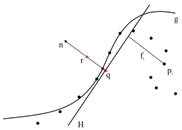
Figure 3: The MLS projection procedure: First, a local reference domain H for the purple point r is generated. The projection of r onto H defines its origin q (the red point). Then, a local polynomial approximation g to the heights f_iof points p_iover H is computed. In both cases, the weight for each of the p_i is a function of the distance to q (the red point). The projection of r onto g (the blue point) is the result of the MLS projection procedure.

system uses an extension of DeFloriani et al’s Multi-Triangulation data structure [15, 16]. A similar system has been developed by Chen and Nguyen [8] as an extension of QSplat.

3

Defining the surface - projecting

Our approach relies on the idea that the given point set implicitly defines a surface. We build upon recent work by Levin [33]. The main idea is the definition of a projection procedure, which projects any point near the point set onto the surface. Then, the MLS surface is defined as the points projecting onto themselves. In the follow-ing, we explain the projection procedure, prove the projection and manifold properties, motivate the smoothness conjecture, and, give details on how to efficiently compute the projection.

3.1 The projection procedure

Let points p_i∈R3,i∈ {1, . . . ,N}, be sampled from a surface S (pos-sibly with a measurement noise). The goal is to project a point r∈R3near S onto a two-dimensional surface SPthat approximates the p_i. The following procedure is motivated by differential ge-ometry, namely that the surface can be locally approximated by a function.

1. Reference domain: Find a local reference domain (plane) for r (see Figure 3). The local plane H={x|hn,xi −D=0,x∈ R3},n∈R3,knk=1 is computed so as to minimize a local weighted sum of square distances of the points p_ito the plane. The weights attached to p_iare defined as the function of the distance of p_ito the projection of r on the plane H, rather than the distance to r. Assume q is the projection of r onto H, then H is found by locally minimizing

N

∑

hn,p_ii −D2θ kp_i−qk

(1) whereθis a smooth, monotone decreasing function, which is positive on the whole space. By setting q=r+tn for some t∈R, (1) can be rewritten as:

N

∑

n,p_i−r−tn2θ kp_i−r−tnk

We define the operatorQ(r) =q=r+tn as the local mini-mum of Eq. 2 with smallest t and the local tangent plane H near r accordingly. The local reference domain is then given by an orthonormal coordinate system on H so that q is the origin of this system.

2. Local map: The reference domain for r is used to compute a local bivariate polynomial approximation to the surface in a neighborhood of r (see Figure 3). Let q_ibe the projection of p_ionto H, and f_ithe height of p_iover H, i.e f_i=n·(p_i−q). Compute the coefficients of a polynomial approximation g so that the weighted least squares error

N

∑

g(x_i,y_i)−f_i2

θ kp_i−qk

(3)

is minimized. Here(x_i,y_i)is the representation of q_iin a lo-cal coordinate system in H. Note that, again, the distances used for the weight function are from the projection of r onto H. The projection P of r onto S_P is defined by the polynomial value at the origin, i.e. P(r) =q+g(0,0)n= r+ (t+g(0,0))n.

3.2 Properties of the projection procedure

In our application scenario the projection property (i.e.

P(P(r)) = P(r)) is extremely important: We want to use the above procedure to compute points exactly on the surface. The implication of using a projection operator is that the set of points we project and the order of the points we project do not change the surface.

From Eq. 2 it is clear that if(t,n)is a minimizer for r then(s,n) is a minimizer for r+ (s−t)n. Assuming the minimization is global in a neighborhood U∈R3of q thenQis a projection operation in U , because the pair(0,n)is a minimizer for r−tn=q. Further, also q+g(0,0)n=r+ (t+g(0,0))n is a minimizer and, thus, also

Pa projection in U .

We like to stress that the projection property results from using distances to q rather than r. Ifθdepended on r the procedure would not be a projection because the values ofθwould change along the normal direction.

The surface S_P is formally defined as the subset of all points inR3 that project onto themselves. A simple counting argument shows that this subset is a two-parameter family and, thus, S_P a 2-manifold. Eq. 2 essentially has 6 degrees of freedom: 3 for r, 2 for n, and 1 for t. On the other hand there are 4 independent necessary conditions: For a local minimum the partial derivatives of the normal and t have to be zero and for r to be on the surface t=0 is necessary. This leaves 6−4=2 free parameters for the surface. It is clear from simple examples that the parameter family includes manifolds which cannot be expressed as functions overR2. The particular charm of this surface definition is that it avoids piecewise parameterizations. No subset of the surface is parameter-ized over a planar piece but every single point has its own support plane. This avoids the common problems of piecewise parameteri-zations for shapes, e.g. parameterization dependence, distortions in the parameterization, and continuity issues along the boundaries of pieces.

However, in this approach we have the problem of proving con-tinuity for any point on the surface because its neighbors have dif-ferent support planes in general. The intuition for S_P∈C∞ is, of course, that (1) interpreted as a functionR6→Ris C∞so that also a particular kernel of its gradient is C∞.

The approximation of single points is mainly dictated by the ra-dial weight functionθ. The weight function suggested in [33] is a

Gaussian

θ(d) =e−

d2

h2 (4)

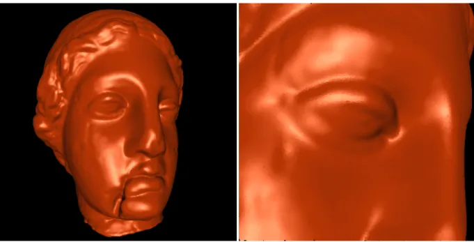
where h is a fixed parameter reflecting the anticipated spacing be-tween neighboring points. By changing h the surface can be tuned to smooth out features of size<h in S. More specifically, a small value for h causes the Gaussian to decay faster and the approxima-tion is more local. Conversely, large values for h result in a more global approximation, smoothing out sharp or oscillatory features of the surface. Figure 4 illustrates the effect of different h values.

3.3 Computing the projection

We explain how to efficiently compute the projection and what val-ues should be chosen for the polynomial degree and h. Furthermore, we discuss trade-offs between accuracy and speed.

Step 1 of the projection procedure is a non-linear optimization problem. Usually, Eq. 2 will have more than one local minimum. By definition, the local minimum with smallest t has to be chosen, which means the plane should be close to r. For minimizing (2) we have to use some iterative scheme, which descends toward the next local minimum. Without any additional information we start with t=0 and first approximate the normal. Note that in this case the weightsθ_i=θ kp_i−rk

are fixed. Let B={b_jk},B∈R3×3 the matrix of weighted covariances be defined by

b_jk=

∑

θ_i

p_i

j−rj pik−rk

.

Then, the minimization problem (2) can be rewritten in bilinear form

min knk=1n

T

Bn (5)

and the solution of the minimization problem is given as the Eigen-vector of B that corresponds to the smallest Eigenvalue.

If a normal is computed (or known in advance) it is fixed and the function is minimized with respect to t. This is a non-linear min-imization problem in one dimension. In general, it is not solvable with deterministic numerical methods because the number of min-ima is only bounded by the number N of points p_i. However, in all practical cases we have found that for t∈[−h/2,h/2]there is only one local minimum. This is intuitively clear as h is connected to the feature size and features smaller than h are smoothed out, i.e. fea-tures with distance smaller than h do not provide several minima. For this reason we make the assumption that any point r to be pro-jected is at most h/2 away from its projection. In all our practical applications this is naturally satisfied.

Using these prerequisites the local minimum is bracketed with ±h/2. The partial derivative

2 N

∑

n,p_i−r−tn 1+

n,p_i−r−tn2 h2

!

ekpi−r−tnk2/h2 ₍₆₎

can be easily evaluated together with the function itself. The deriva-tive is exploited in a simple iteraderiva-tive minimization scheme as ex-plained in [43, Chapter 10.3].

Once t6=0 fixing t and minimization with respect to the normal direction is also a non-linear problem because q=r+tn changes and, thus, also the weights change. The search space can be visual-ized as the tangent planes of a sphere with center point r and radius t. However, in practice we have found the normal (or q) to change only slightly so that we approximate the sphere locally around the current value of r+tn as the current plane defined t and n. On this plane a conjugate gradient scheme [43] is used to minimize among

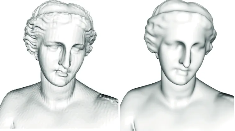
Figure 4: The effect of different values for parameter h. A point set representing an Aphrodite statue defines an MLS surface. The left side shows an MLS surface resulting from a small value and reveals a surface micro-structure. The right side shows a larger value for h, smoothing out small features or noise.

all q on the plane. The main idea is to fix a subspace for minimiza-tion in which n cannot vanish so that the constraintknk=1 is al-ways satisfied. The use of a simple linear subspace makes the com-putation of partial derivatives efficient and, thus, conjugate gradient methods applicable. Clearly, this search space effectively changes t resulting in a theoretically worse convergence behavior. In prac-tice, the difference between the sphere and the plane is small for the region of interest and the effect is not noticeable.

Using these pieces the overall implementation of computing the support plane looks like this:

Initial normal estimate in r: The normal in a point might be

given as part of the input (e.g. estimate from range images) or could be computed when refining a point set surface (e.g. from close points in the already processed point set). If no normal is available it is computed using the Eigenvector of the matrix of weighted co-variances B.

Iterative non-linear minimization: The following two steps are

repeated as long as any of the parameters changes more than a predefinedε:

1. Minimize along t, where the minimum is initially brack-eted by t=±h/2.

2. Minimize q on the current plane H :(t,n)using conju-gate gradients. The new value for q=r+tn leads to new values for the pair(t,n).

The last pair(t,n)defines the resulting support plane H.

The second step of the projection procedure is a standard linear least squares problem: Once the plane H is computed, the weights θ_i=θ(kp_i−qk)are known. The gradient of (3) over the unknown

coefficients of the polynomial leads to a system of linear equations of size equal to the number of coefficients, e.g. 10 for a third degree polynomial.

Through experimentation, we found that high degree polynomi-als are likely to oscillate. Polynomipolynomi-als of degree 3 to 4 have proved to be very useful as they produce good fits of the neighborhood, do not oscillate, and are quickly computed.

3.4 Data structures and trade-offs

The most time-consuming step in computing the projection of a point r is collecting the coefficients from each of the p_i(i.e. com-puting the sum). Implemented naively, this process takes O(N) time, where N is the number of points. We exploit the effect of the quickly decreasing weight function in two ways:

1. In a certain distance from r the weight function is effectively zero. We call this the neglect distance dn, which depends solely on h. A regular grid with cell size 2dnis used to parti-tion the point set. For each projecparti-tion operaparti-tion a maximum of 8 cells is needed. This results in a very small memory foot print and yields a simple and effective out of core implemen-tation, which makes the storage requirements of this approach independent of the total size of the point set.

2. Using only the selected cells the terms are collected using a hierarchical method inspired by solutions to the N-body prob-lem [4]. The basic observation is, that a cluster of points far from r can be combined into one point. To exploit this idea, each cell is organized as an Octree. Leaf nodes contain the p_i; inner nodes contain information about the number of points in the subtree and their centroid. Then, terms are collected

from the nodes of the Octree. If the node’s dimension is much smaller than its distance to r, the centroid is used for com-puting the coefficients; otherwise the subtree is traversed. In addition, whole nodes can be neglected if their distance to r is larger than dn.

The idea of neglecting points could be also made independent of numerical issues by using a compactly supported weight function. However, the weight function has to be smooth. An example for such an alternative isθ(x) =2x3−3x2+1.

A simple way to trade accuracy for speed is to assume that the plane H passes through the point to be projected. This assumption is reasonable for input points, which are expected to be close to the surface they define (e.g. input that has been smoothed). This simplification saves the cost of the iterative minimization scheme. 3.5 Results

Actual timings for the projection procedure depend heavily on the feature size h. On a standard Pentium PC the points of the bunny were projected at a rate of 1500-3500 points per second. This means the 36K points of the bunny are projected onto the surface they define themselves in 10-30 seconds. Smaller values for h lead to faster projection since the neighborhoods and, thus, the number of points taken into account are smaller.

As has been stressed before, the memory requirements mainly depend on the local feature size h. As long as h is small with respect to the total diameter of the model the use of main memory of the projection procedure is negligible.

4

Approximation error

Consider again the setting depicted in Figure 2. Input points{p_i} define a surface S_P, which are then represented by a set of points {r_i} ∈S_P. However, the set{r_i}defines a surface S_Rwhich approx-imates S_P. Naturally, we would like to have an upper bound on the distance between S_Rand S_P.

From differential geometry, we know that a smooth surface can be locally represented as a function over a local coordinate sys-tem. We also know that in approximating a bivariate function f by a polynomial g of total degree m, the approximation error is kg−fk ≤M·hm+1_{[32]. The constant M involves the(m+1)-th} derivatives of f , i.e. M∈O(kf(m+1)k). In the case of surface ap-proximation, since S_Pis infinitely smooth, there exists a constant M_m+1, involving the(m+1)-th derivatives of S_P, such that

kS_P−S_Rk ≤M_m+1hm+1 (7) where S_Ris computed using polynomials of degree m.

Note that this error bound holds for the MLS surface S_R, which is obtained by the projection procedure applied to the data set R, using the same parameter h as for S_P. Moreover, the same type of approximation order holds for piecewise approximation: Assume each point r_idefines a support plane so that S_P is a function over a patch[−h,h]2_{around r}

ion the plane and, further, that the points {r_i}leave no hole of radius more than h on the surface. Then, the above arguments hold and the approximation error of the union of local, non-conforming, polynomial patches G_iaround points r_i approximates S_Pas

SP−

[ G_i

≤Mm+1h

m+1_{. (8)}

Here, G_iis the polynomial patch defined by an MLS polyno-mial g_ifor the point r_i, with corresponding reference plane H_iwith

(a)

(b)

(c)

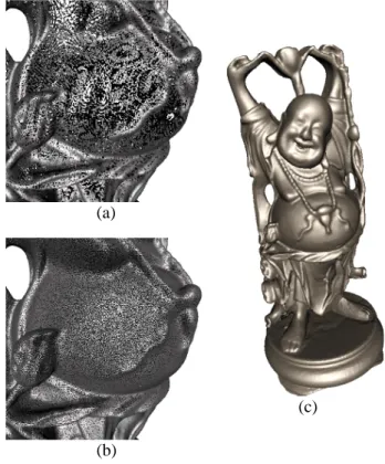
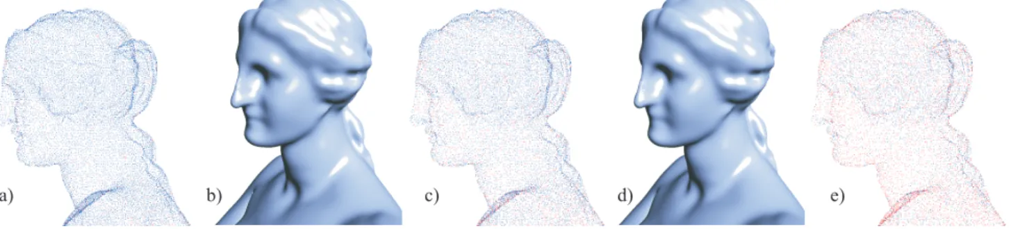
Figure 5: Points acquired by range scanning devices or vertices from a processed mesh typically have uneven sampling density on the surface (a). The sampling techniques discussed here allow to evenly re-sample the object (b) to ensure a sufficient density for further processing steps, for example rendering (c).

normal n_i, a corresponding orthonormal system{u_i,v_i,n_i}, and an origin at q_i.

G_i={q_i+x·u_i+y·v_i+g_i(x,y)·n_i|(x,y)∈[−h,h]2}. (9) These error bounds explain nicely why curvature (see e.g. [17]) is an important criterion for piecewise linear approximations (meshes): The error of piecewise linear functions depends linearly on the second derivatives and the spacing of points. This means, more points are needed where the curvature is higher.

However, when the surface is approximated with higher order polynomials, curvature is irrelevant to the approximation error. Us-ing cubic polynomials, the approximation error depends on the fourth order derivatives of the surface. Note that our visual sys-tem cannot sense smoothness beyond second order [38]. From that point of view, the sampling density locally depends on an “invisi-ble” criterion. We have found it to be sufficient to fix a spacing h of points r_ion S_P. A smaller h will cause the error to be smaller. However, using higher order polynomials to approximate S_Pcauses the error to decrease faster when h is reduced.

5

Generating the representation point set

The problem of noise is handled by projecting the points onto the MLS surface they define. The result of the projection proce-dure is a thin point set. Redundancy is avoided by decimating the

a)

b)

Figure 6: Noisy input points (green points) are projected onto their smooth MLS curve (orange points). The figures in (a) show the point sets and a close-up view. The decimation process is shown in (b). Points are color-coded as in Figure 7.

point set, taking care that it persists to be a good approximation of the MLS surface defined by the original point set. In the case of under-sampling, the input point set needs to be up-sampled. In the following sections, we show techniques to remove and add points.

Figure 5 illustrates the idea of re-sampling at the example of the Buddha statue. Using the techniques presented below it is possible to re-sample the geometry to be evenly sampled on the surface. 5.1 Down-sampling

Given a point set, the decimation process repeatedly removes the point that contributes the smallest amount of information to the shape. The contribution of a point to the shape or the error of the sampling is dictated by the definition of the shape. If the point set is reconstructed by means of a triangulation, criteria from the specific triangulation algorithm should control the re-sampling. Criteria in-clude the distance of points on the surface [23], curvature [17], or distance from the medial axis of the shape [2]. For a direct display of the point set on a screen homogeneous distribution of the points over the surface is required [19, 41]. Here, we derive a criterion motivated by our definition of the surface.

The contribution of a projected point p_ito the surface S_P can be estimated by comparing S_Pwith S_P−{p

i}

. Computing the Haus-dorff distance between both surfaces is expensive and not suitable for an iterative removal of points of a large point set. Instead, we approximate the contribution of p_iby its distance from its projec-tion onto the surface S_P−{p

i}. Thus, we estimate the difference of

S_Pand S_P−{p

i}by projecting pionto SP−{pi}(projecting piunder

the assumption it was not part of P).

The contribution values of all points are inserted into a priority queue. At each step of the decimation process, the point with the smallest error is removed from the point set and from the priority queue. After the removal of a point, the error values of nearby points have to be recalculated since they might have been affected by the removal. This process is repeated until the desired number of points is reached or the contributions of all points exceed some prespecified bound.

Figure 6 illustrates our decimation process applied on the set of red points depicted in (a). First, the red points are projected on the MLS surface to yield the blue points. A close-up view over a part of the points shows the relation between the input (red) points and the projected points. In (b), we show three snapshots of the decimation process, where points are colored according to their error value; blue represents low error and red represents high error. Note that

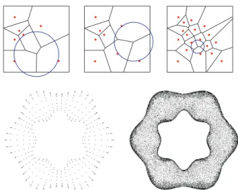
Figure 8: The up-sampling process: Points are added at vertices of the Voronoi diagram. In each step, the vertex with the largest empty circle is chosen. The process is repeated until the radius of the largest circle is smaller than a specified bound. The wavy torus originally consisting of 800 points has been up-sampled to 20K points.

in the sparsest set, all of the points have a high error, that is, their removal will cause a large error. As the decimation proceeds, fewer points remain and their importance grows and the error associated with them is larger. Figure 7 shows the decimation process in 3D with corresponding renderings of the point sets.

5.2 Up-sampling

In some cases, the density of the point set might not be sufficient for the intended usage (e.g. direct point rendering or piecewise recon-structions). Motivated by the error bounds presented in Section 4 we try to decrease the spacing among points. Additional points should be placed (and then projected to the MLS surface) where the spacing among points is larger then a specified bound.

The basic idea of our approach is to compute Voronoi diagrams on the MLS surface and add points at vertices of this diagram. Note that the vertices of the Voronoi diagram are exactly those points on the surface with maximum distance to several of the existing points. This idea is related to Lloyd’s method [37], i.e techniques using Voronoi diagrams to achieve a certain distribution of points [40].

However, computing the Voronoi diagram on the MLS surface is excessive and local approximations are used instead. More specif-ically, our technique works as follows: In each step, one of the ex-isting points is selected randomly. A local linear approximation is built and nearby points are projected onto this plane. The Voronoi diagram of these points is computed. Each Voronoi vertex is the center of a circle that touches three or more of the points without including any point. The circle with largest radius is chosen and its center is projected to the MLS surface. The process is repeated iteratively until the radius of the largest circle is less than a user-specified threshold. (see Figure 8). At the end of the process, the density of points is locally near-uniform on the surface. Figure 8 shows the original sparse point set containing 800 points, and the same object after adding 20K points over its MLS surface.

e) d)

c)

a) b)

Figure 7: The point set representing an Aphrodite statue is projected onto a smooth MLS-surface. After removing redundant points, a set of 37K points represents the statue (a). The corresponding rendering is shown in (b). The point set is decimated using point removal. An intermediate stage of the reduction process is shown in (c). Note that the points are color-coded with respect to their importance. Blue points do not contribute much to the shape and might be removed; red points are important for the definition of the shape. The final point set in (e) contains 20K points. The corresponding rendering is depicted in (d) and is visually close to the one in (b).

6

Rendering

The challenge of our interactive point rendering approach is to use the representation points and (when necessary) create new points by sampling the implicitly defined surface at a resolution sufficient to conform to the screen space resolution (see Figure 9 for an illus-tration of that approach).

Usually, the representation points are not sufficient to render the object in screen space. In some regions, it is not necessary to render all points as they are occluded, backfacing, or have higher density than needed. However, typically, points are not dense enough to be projected directly as a single pixel and more points need to be generated by interpolation in object space.

6.1 Culling and view dependency

The structure of our rendering system is similar to QSplat [46]. The input points are arranged into a bounding sphere hierarchy. For each node, we store a position, a radius, a normal coverage, and option-ally a color. The leaf nodes additionoption-ally store the orientation of the support plane and the coefficients of the associated polynomial. The hierarchy is used to cull the nodes with the view frustum and to apply a hierarchical backface culling [29]. Note that culling is im-portant for our approach since the cost of rendering the leaf nodes (evaluating the polynomials) is relatively high compared to simpler primitives. Moreover, if the traversal reaches a node with an extent that projects to a size of less than a pixel, this node is simply pro-jected to the frame-buffer without traversing its subtree. When the traversal reaches a leaf node and the extent of its bounding sphere projects to more than one pixel in screen space, additional points have to be generated.

The radius of a bounding sphere in leaf nodes is simply set to the anticipated feature size h. The bounding spheres for inner nodes naturally bound all of their subtree’s bounding spheres. To compute the size of a bounding sphere in pixel space the radius is scaled by the model-view transform and then divided by the distance of center and eye point in z-direction to accommodate the projective transform.

6.2 Sampling additional points

The basic idea is to generate a grid of points sufficient to cover the extent of a leaf node. However, projecting the grid points using the method described in Section 3 is too slow in interactive appli-cations. The main idea of our interactive rendering approach is to sample the polynomials associated with the representation points rather than really projecting the points.

h

Figure 10: The patch size of a polynomial: Points inside a ball of radius h around the red point r are projected onto the support plane of the red point. The patch size is defined as the bounding disk (in local coordinates) of the projections. Note that using a disk of radius h would lead to unpleasant effects in some cases, as the polynomial might leave the ball of radius h.

It is clear that the union of these polynomial patches is not a continous surface. However, the Hausdorff-error of this approxi-mation is not worse than the error of the surface computed by pro-jecting every point using the operatorP(see Section 4). Since the Hausdorff-error in object space limits the screen space error the er-ror bound can be used to make the approximation erer-ror invisble in the resulting image.

However, to conform with the requirements formulated in Sec-tion 4 the point set and the associated polyonmials are required to be near-uniform on the surface. It might be necessary to first pro-cess a given point set with the up-sampling methods presented in Section 5. This way, we ensure that the local, non-conforming (i.e. overlapping or intersecting) polynomials are a good approximation to the surface inside a patch[−h,h]2around a point and, thus, the re-sulting image shows a smooth surface. However, most dense point sets can be readily displayed with the approach presented here. For example, Figure 11 shows several renderings of the original Stan-ford Bunny data.

It is critical to properly define the extent of a polynomial patch on the supporting plane, such that neighboring patches are guaranteed to overlap (to avoid holes) but do not overlap more than necessary. Since no inter-point connectivity information is available, it is un-clear which points are immediate neighbors of a given point on the surface.

To compute the extent of a polynomial patch associated to the point p_i on the support plane H all points inside a ball of radius

Figure 9: Up-sampling could be used generate enough points on the surface to conform with the resolution of the image to be rendered. The right image shows a close-up rendered with splats.

h around the projection q=Q(p_i)are collected. These points are projected to the support plane H, which leads to local(u,v) coor-dinates for each projected point. The extent is defined by a circle around q that encloses all projected points. More specifically, as-sume q has the local coordinate (0,0), the radius of the circle is given by the largest 2-norm of all local(u,v)coordinates of pro-jected points. Since the spacing of points is expected to be less than h, patches of neighboring points are guaranteed to overlap.

Note that using a constant extent (e.g. a disk of radius h on the support plane) can lead to errors, as the polynomial g over H might leave the ball of radius h, in which a good approximation of the point set is expected. Figure 10 illustrates the computation of the patch sizes.

The grid spacing d should be so computed that neighboring points have a screen space distance of less than a pixel. Thus, the grid spacing depends on the orientation of the polyonmial patch with respect to the screen. Since the normals change on each poly-onmial patch we rather use a simple heuristic to conservatively esti-mate d: The grid spacing d is computed so that a grid perpendicular to the viewing direction is sufficiently sampled in image space.

If the grid is, indeed, perpendicular to the viewing direction, the sampling is also correct on the polynomial. If the grid is not perpen-dicular to the viewing direction, the projected area might be over-sampled or underover-sampled depending on the orientation of the sup-port plane and the derivatives of the polyonmial. Note, however, that sufficient sampling is guaranteed if the derivatives are less than 1. In practice we have rarely encountered higher derivatives so we decided not to evaluate the maximum derivatives of all polynomial patches. However, this could be done in a preprocess and the den-sity could be adjusted accordingly.

Upon the view-dependent grid spacing d, the polynomials are evaluated by a forward difference approach, where the polynomial is scanned across its extent in its local u,v parametric space. The affine map transforming from support plane coordinates to world coordinates is factored into polynomial evaluation, thus, generat-ing points in world coordinates. These points are then fed into the graphics pipeline to be projected to the screen.

Surprisingly, we have found that quad meshes are processed

faster by current graphics hardware than a set of points. For this reason we use quad meshes to represent the polynomial patches. This has the additional advantage that during lazy evaluation (see below) no holes occur.

6.3 Grid pyramids

The time-critical factor is the view-dependent evaluation of the points on the polynomial. Optimally, these are recomputed when-ever the projected screen space size changes. To accelerate the ren-dering process, we store a grid pyramid with various resolutions per representation point. Initially, the pyramid levels are created, but no grid is actually evaluated. When a specific grid resolution is needed, the system creates and stores the level that slightly oversamples the polynomial for a specific resolution, such that small changes in the viewing position do not result in new evaluations.

To enhance the interactivity of our approach we use lazy evalua-tion during rotating or zooming. Once the viewer stops moving, a proper grid is chosen from the pyramid.

6.4 Results

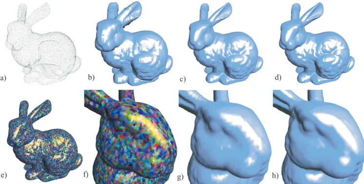
We have tested our approach on a variety of point sets. Figure 11 shows the renderings of the Stanford Bunny. In (a), the original point set is shown. Splatting (b) is not leading to good results, be-cause the model is not sampled densely enough. The traditional Gouraud-shaded mesh in (c) and (g) is compared to our approach in (d) and (h). Note the accuracy of the highlights. The non-conforming local polynomial patches are shown color-coded in (e) and (f). An example of a environment mapping to demonstrate the normal continuity is given in Figure 12. Note that silhouettes and normals are smooth, which leads to less distortions on the boundary and in the reflections.

The frame rates we achieve are mainly dictated by the number of visible representation points (i.e. graph traversal time) and the number of pixels to be filled. All models depicted in the paper are displayed at more than 5 frames per second in a 5122 screen window (see the accompanying video for more information). The

a)

b)

_c)

d)

e)

f)

_g)

h)

Figure 11: The Stanford Bunny: The points defining the bunny are depicted in (a) (some points are culled). Points are splatted in (b) to satisfy screen space resolution. Note the difference of a piecewise linear mesh over the points (c) and close-up in (g) to the rendering of non-conforming polynomial patches (d) and (h). The patches are color-coded in (e) and (f).

number of representation points ranges from 1000 (for the torus) to 900K (for the angel statue). Tests are performed on a PC with GeForce2 graphics board.

7

Conclusion

In differential geometry, a smooth surface is characterized by the existence of smooth local maps at any point. In this work we use this as a framework to approximate a smooth surface defined by a set of points and we introduced new techniques to resample the surface to generate an adequate representation of the surface.

To render such surfaces, the surface is covered by a finite num-ber, as small as possible, of non-conforming, overlapping, polyno-mial patches. We showed that the error of these approximations is bounded and dependent on the spacing among points. Thus, it is possible to provide a point set representation that conforms with a specified tolerance.

Our paradigm for representing surfaces advocates the use of a point set (without connectivity) as a representation of shapes. This representation is universal in the sense that it is used from the be-ginning (i.e. acquisition) to the end (i.e. rendering) of a graphical representation’s life cycle. Moreover, we believe that this work is a step towards rendering with higher order polynomials. Note that we have used simple primitives (points) to achieve this goal. This admits to the current trend of integrating high quality rendering fea-tures into graphics hardware.

It would be interesting to integrate our approach with combina-torial methods such as the one of Amenta et al [2]. This would com-bine topological guarantees with the additional precision of higher order approximations and the possibility of smoothing out noise or small features.

Using different values for h, it is easy to generate more smooth or more detailed versions of a surface from one point set (see, for

Figure 12: Comparison of mesh rendering with our technique with environment mapping. The left column shows renderings of a mesh consisting of 1000 vertices. The right column shows our technique using the vertices as input points. The environment maps empha-size the improved normal and boundary continuity.

example, Figure 4). A set of different versions could be used as a smooth-to-detailed hierarchy and would allow for multiresolution modeling [27]. Of course, h is not necessarily a global parameter and could be adapted to the local feature size. Varying h has sev-eral implications and utility in handling point sets (see [30] for a nice introduction to the issues in two dimensions), such as prop-erly accounting for differences in sampling rate and levels of noise during the acquisition process. Also, non radial functions might be necessary to properly account for sharp features in the models.

Acknowledgements

We gratefully acknowledge the helpful comments of Markus Gross, J¨org Peters, Ulrich Reif, and several anonymous reviewers.

This work was supported by a grant from the Israeli Ministry of Science, a grant from GIF (German Israeli Foundation) and a grant from the Israeli Academy of Sciences (center of excellence). The bunny model is courtesy of the Stanford Computer Graphics Labo-ratory. The angel statue in Figure 1 was scanned by Peter Neuge-bauer at Fraunhofer IGD in Darmstadt, Germany using a structured light scanner and the QTSculptor system.

References

[1] M. Alexa, J. Behr, D. Cohen-Or, S. Fleishman, D. Levin, and C. T. Silva. Point set surfaces. In IEEE Visualization 2001, pages 21–28, October 2001. ISBN 0-7803-7200-x.

[2] N. Amenta, M. Bern, and M. Kamvysselis. A new voronoi-based surface recon-struction algorithm. Proceedings of SIGGRAPH 98, pages 415–422, July 1998. [3] C. L. Bajaj, F. Bernardini, and G. Xu. Automatic reconstruction of surfaces

and scalar fields from 3d scans. Proceedings of SIGGRAPH 95, pages 109–118, August 1995.

[4] J. Barnes and P. Hut. A hierarchical O(N log N) force calculation algorithm. Nature, 324:446–449, Dec. 1986. Technical report.

[5] F. Bernardini, J. Mittleman, H. Rushmeier, C. Silva, and G. Taubin. The ball-pivoting algorithm for surface reconstruction. IEEE Transactions on Visualiza-tion and Computer Graphics, 5(4):349–359, October - December 1999. [6] P. Besl and N. McKay. A method for registration of 3-d shapes. IEEE

Transaltions on Pattern Analysis and Machine Intelligence, 14(2):239–256, February 1992.

[7] J.-D. Boissonnat. Geometric structues for three-dimensional shape representa-tion. ACM Transactions on Graphics, 3(4):266–286, October 1984.

[8] B. Chen and M. X. Nguyen. Pop: a hybrid point and polygon rendering system for large data. In IEEE Visualization 2001, pages 45–52, October 2001. ISBN 0-7803-7200-x.

[9] P. Cignoni, C. Montani, and R. Scopigno. A comparison of mesh simplification algorithms. Computers & Graphics, 22(1):37–54, February 1998.

[10] J. D. Cohen, D. G. Aliaga, and W. Zhang. Hybrid simplification: combining multi-resolution polygon and point rendering. In IEEE Visualization 2001, pages 37–44, October 2001. ISBN 0-7803-7200-x.

[11] P. Crossno and E. Angel. Isosurface extraction using particle systems. IEEE Visualization ’97, pages 495–498, November 1997.

[12] B. Curless and M. Levoy. A volumetric method for building complex models from range images. Proceedings of SIGGRAPH 96, pages 303–312, August 1996.

[13] L. H. de Figueiredo, J. de Miranda Gomes, D. Terzopoulos, and L. Velho. Physically-based methods for polygonization of implicit surfaces. Graphics In-terface ’92, pages 250–257, May 1992.

[14] M. Desbrun, M. Meyer, P. Schr¨oder, and A. H. Barr. Implicit fairing of irregular meshes using diffusion and curvature flow. Proceedings of SIGGRAPH 99, pages 317–324, August 1999.

[15] L. D. Floriani, P. Magillo, and E. Puppo. Building and traversing a surface at variable resolution. IEEE Visualization ’97, pages 103–110, November 1997. ISBN 0-58113-011-2.

[16] L. D. Floriani, P. Magillo, and E. Puppo. Efficient implementation of multi-triangulations. IEEE Visualization ’98, pages 43–50, October 1998. ISBN 0-8186-9176-X.

[17] M. Gopi, S. Krishnan, and C. T. Silva. Surface reconstruction based on lower dimensional localized delaunay triangulation. Computer Graphics Forum, 19(3), August 2000.

[18] A. Goshtasby and W. D. O’Neill. Surface fitting to scattered data by a sum of gaussians. Computer Aided Geometric Design, 10(2):143–156, April 1993. [19] J. P. Grossman and W. J. Dally. Point sample rendering. Eurographics Rendering

Workshop 1998, pages 181–192, June 1998.

[20] A. P. Gueziec, G. Taubin, F. Lazarus, and W. Horn. Converting sets of polygons to manifold surfaces by cutting and stitching. IEEE Visualization ’98, pages 383–390, October 1998.

[21] P. Hebert, D. Laurendeau, and D. Poussart. Scene reconstruction and descrip-tion: Geometric primitive extraction from multiple view scattered data. In IEEE Computer Vision and Pattern Recognition 1993, pages 286–292, 1993. [22] H. Hoppe, T. DeRose, T. Duchamp, M. Halstead, H. Jin, J. McDonald,

J. Schweitzer, and W. Stuetzle. Piecewise smooth surface reconstruction. Pro-ceedings of SIGGRAPH 94, pages 295–302, July 1994.

[23] H. Hoppe, T. DeRose, T. Duchamp, J. McDonald, and W. Stuetzle. Surface reconstruction from unorganized points. Computer Graphics (Proceedings of SIGGRAPH 92), 26(2):71–78, July 1992.

[24] H. Hoppe, T. DeRose, T. Duchamp, J. McDonald, and W. Stuetzle. Mesh opti-mization. Proceedings of SIGGRAPH 93, pages 19–26, August 1993. [25] A. Kalaiah and A. Varshney. Differential point rendering. In Rendering

Tech-niques 2001: 12th Eurographics Workshop on Rendering, pages 139–150. Euro-graphics, June 2001. ISBN 3-211-83709-4.

[26] A. Kaufman, D. Cohen, and R. Yagel. Volume graphics. IEEE Computer, 26(7):51–64, July 1993.

[27] L. P. Kobbelt, T. Bareuther, and H.-P. Seidel. Multiresolution shape deforma-tions for meshes with dynamic vertex connectivity. Computer Graphics Forum, 19(3):249–259, Aug. 2000.

[28] V. Krishnamurthy and M. Levoy. Fitting smooth surfaces to dense polygon meshes. Proceedings of SIGGRAPH 96, pages 313–324, August 1996. [29] S. Kumar, D. Manocha, W. Garrett, and M. Lin. Hierarchical back-face

compu-tation. In X. Pueyo and P. Schr¨oder, editors, Eurographics Rendering Workshop 1996, pages 235–244, New York City, NY, June 1996. Eurographics, Springer Wien.

[30] I.-K. Lee. Curve reconstruction from unorganized points. Computer Aided Geo-metric Design, 17(2):161–177, February 2000.

[31] Z. Lei, M. M. Blane, and D. B. Cooper. 3L fitting of higher degree implicit poly-nomials. In Proceedings of Third IEEE Workshop on Applications of Computer Vision, Sarasota, Florida, USA, Dec. 1996.

[32] D. Levin. The approximation power of moving least-squares. Mathematics of Computation, 67(224), 1998.

[33] D. Levin. Mesh-independent surface interpolation. Advances in Computational Mathematics, in press, 2001.

[34] M. Levoy, K. Pulli, B. Curless, S. Rusinkiewicz, D. Koller, L. Pereira, M. Ginz-ton, S. Anderson, J. Davis, J. Ginsberg, J. Shade, and D. Fulk. The digital michelangelo project: 3d scanning of large statues. Proceedings of SIGGRAPH 2000, pages 131–144, July 2000.

[35] M. Levoy and T. Whitted. The use of points as a display primitive. Tr 85-022, University of North Carolina at Chapel Hill, 1985.

[36] L. Linsen. Point cloud representation. Technical report, Fakult¨at fuer Informatik, Universit¨at Karlsruhe, 2001.

[37] S. P. Lloyd. Least squares quantization in PCM. IEEE Transactions on Informa-tion Theory, 28:128–137, 1982.

[38] D. Marr. Vision: A Computational Investigation into the Human Representation and Processing of Visual Information. W. H. Freeman, Sept. 1983.

[39] D. K. McAllister, L. F. Nyland, V. Popescu, A. Lastra, and C. McCue. Real-time rendering of real-world environments. Eurographics Rendering Workshop 1999, June 1999.

[40] A. Okabe, B. Boots, and K. Sugihara. Spatial Tesselations — Concepts and Applications of Voronoi Diagrams. Wiley, Chichester, 1992.

[41] H. Pfister, M. Zwicker, J. van Baar, and M. Gross. Surfels: Surface elements as rendering primitives. Proceedings of SIGGRAPH 2000, pages 335–342, July 2000.

[42] V. Pratt. Direct least-squares fitting of algebraic surfaces. Computer Graphics (Proceedings of SIGGRAPH 87), 21(4):145–152, July 1987.

[43] W. H. Press, S. A. Teukolsky, W. T. Vetterling, and B. P. Flannery. Numerical Recipes in C: The Art of Scientific Computing (2nd ed.). Cambridge University Press, 1992.

[44] R. Ramamoorthi and J. Arvo. Creating generative models from range images. Proceedings of SIGGRAPH 99, pages 195–204, August 1999.

[45] S. Runsinkiewicz and M. Levoy. Streaming qsplat: A viewer for networked visualization of large, dense models. In to appear in Proceedings of Symposium on Interactive 3D Graphics. ACM, 2001.

[46] S. Rusinkiewicz and M. Levoy. Qsplat: A multiresolution point rendering system for large meshes. Proceedings of SIGGRAPH 2000, pages 343–352, July 2000. [47] M. Rutishauser, M. Stricker, and M. Trobina. Merging range images of arbitrarily

shaped objects. In IEEE Computer Vision and Pattern Recognition 1994, pages 573–580, 1994.

[48] G. Schaufler and H. W. Jensen. Ray tracing point sampled geometry. Rendering Techniques 2000: 11th Eurographics Workshop on Rendering, pages 319–328, June 2000.

[49] M. Soucy and D. Laurendeau. Surface modeling from dynamic integration of multiple range views. In 1992 International Conference on Pattern Recognition, pages I:449–452, 1992.

[50] M. Sramek and A. E. Kaufman. Alias-free voxelization of geometric objects. IEEE Transactions on Visualization and Computer Graphics, 5(3):251–267, July - September 1999. ISSN 1077-2626.

[51] G. Taubin. A signal processing approach to fair surface design. Proceedings of SIGGRAPH 95, pages 351–358, August 1995.

[52] G. Turk. Re-tiling polygonal surfaces. Computer Graphics (Proceedings of SIGGRAPH 92), 26(2):55–64, July 1992.

[53] G. Turk and M. Levoy. Zippered polygon meshes from range images. Proceed-ings of SIGGRAPH 94, pages 311–318, July 1994.

[54] S. W. Wang and A. E. Kaufman. Volume sculpting. 1995 Symposium on Inter-active 3D Graphics, pages 151–156, April 1995. ISBN 0-89791-736-7. [55] M. Wheeler, Y. Sato, and K. Ikeuchi. Consensus surfaces for modeling 3d objects

from multiple range images. In IEEE International Conference on Computer Vision 1998, pages 917–924, 1998.

[56] A. P. Witkin and P. S. Heckbert. Using particles to sample and control implicit surfaces. Proceedings of SIGGRAPH 94, pages 269–278, July 1994.