HAL Id: hal-02102304
https://hal.archives-ouvertes.fr/hal-02102304
Submitted on 17 Apr 2019
HAL
is a multi-disciplinary open access
archive for the deposit and dissemination of
sci-entific research documents, whether they are
pub-lished or not. The documents may come from
teaching and research institutions in France or
abroad, or from public or private research centers.
L’archive ouverte pluridisciplinaire
HAL
, est
destinée au dépôt et à la diffusion de documents
scientifiques de niveau recherche, publiés ou non,
émanant des établissements d’enseignement et de
recherche français ou étrangers, des laboratoires
publics ou privés.
Interpolation Applied to Low-Frequency
Electromagnetic Problem
Thomas Henneron, Antoine Pierquin, Stephane Clénet
To cite this version:
Thomas Henneron, Antoine Pierquin, Stephane Clénet.
Mesh Deformation Based on
Ra-dial Basis Function Interpolation Applied to Low-Frequency Electromagnetic Problem.
IEEE
Transactions on Magnetics, Institute of Electrical and Electronics Engineers, 2019, 14, pp.1-4.
�10.1109/TMAG.2019.2896623�. �hal-02102304�
Mesh Deformation based on Radial Basis Function Interpolation
applied to Low Frequency Electromagnetic Problem
Thomas Henneron
1, Antoine Pierquin
1and St´ephane Cl´enet
11 Univ. Lille, Centrale Lille, Arts et Metiers ParisTech, HEI, EA 2697 - L2EP, F-59000 Lille, France
In order to take into account a modification of the geometry during an optimization process or due to a physical phenomenon, a deformation of the elements of the spatial discretization is preferable to conserve a conformal mesh and to apply the Finite Element (FE) method. To perform the displacement of nodes, interpolation method can be investigated in this context. In this paper, the Radial Basis Function (RBF) interpolation method is applied for low frequency electromagnetic problems solved by the FE method. A 2D magnetostatic example is considered to study the influence of the parameters of the RBF interpolation. To test the extension in 3D, a non destructive testing (NDT) problem is treated where the shape of the crack is modified by applying the proposed method.
Index Terms—mesh deformation, Radial Basis Function, finite element method, low frequency electromagnetism.
I. INTRODUCTION
T
O study low frequency electromagnetic devices, the FE method is widely used. For problems with a parametrized shape or involving dynamic behavior of boundaries (dynamic magneto mechanical behavior for example), the FE mesh should fit the modification of the geometry. To solve this kind of problem, a simple approach consists in remeshing the geometry. Nevertheless, this method is not very efficient be-cause it introduces a numerical noise and it breaks the natural link between two successive solutions in a time dependent problem. Different approaches based on interpolation methods have been developed in order to deform an initial mesh to take into account a shape modification. The idea is to impose the displacement for a set of nodes of the mesh or of points of the geometry and to determine the new coordinates for all other ones by an interpolation approach. In this context, the isogeometric analysis (IGA) [1] and the Radial Basis Function (RBF) interpolation method [2] can be investigated. For low frequency electromagnetic problems, for example, the IGA approach has been applied to optimize the shape of permanent magnets of a synchronous motor [3] or to parametrize the geometry of a piezoelectric device [4].In this article, we propose to use the RBF interpolation method for the mesh deformation in the case of low frequency electromagnetic devices solved by the FE method. Initially, the approach has been developed in the case of flow fluid problem [5]. First, the RBF interpolation method is presented. Sec-ondly, the mesh deformation based on the RBF is described. Thirdly, numerical experiments are performed in order to study the influence of the parameters of the RBF interpolation with a 2D magnetostatic problem. Finally, a 3D non destructive testing device is investigated for different shapes of the crack obtained from the RBF approach.
II. RADIALBASISFUNCTION INTERPOLATION METHOD
The RBF interpolation method is often used to compute an approximation s(x)of a multivariable functionf(x). This
Manuscript received December 1, 2012; revised August 26, 2015. Corre-sponding author: T. Henneron (email: [email protected]).
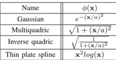
TABLE I EXAMPLES OFRBFFUNCTION Name φ(x) Gaussian e−(x/a)2 Multiquadric p1 + (x/a)2 Inverse quadric q1+(x1/a)2 Thin plate spline x2log(x)
approximation is expressed as a linear combination of basis functionsφ. In a general way, we considerNt training points
such asyi=f(xi)fori= 1, .., Ntwithxi ∈Rpandyi∈R.
Then, for a new coordinatex∈Rp, the approximation off(x)
is given by f(x)≈s(x) = Nt X i=1 αiφi(x) (1) withφi(x) =φ(||x−xi||),
where φi is a radial function depending on the Euclidian
distance betweenxandxi andαiis its associated coefficient.
The coefficientsαi are calculated using theNttraining points
in order to verify yj=f(xj) =s(xj) = Nt X i=1 αiφi(||xj−xi||) (2) for j= 1, .., Nt.
Then, we can define a matrix system to be solved for the computation of αi such as Y=GαwithY= [y1, ..., yNt] t, α= [α 1, ..., αNt] t (3) andG= φ1(x1) . . . φ1(xNt) .. . . .. ... φNt(x1) . . . φNt(xNt) .
The error of interpolation depends on the choice of RBF. Table 1 presents different examples of functions where a is a parameter fixed by the user. Others functions can be used for the RBF interpolation such as functions with compact
support [5]. In the case of vector function f(x) ∈ Rq, the
RBF method is performed for each component off(x). Then, the approximations(x)is f(x)≈s(x) = s1(x) .. . sq(x) withs j(x) = Nt X i=1 αijφi(x) (4) for j= 1, .., q.
In this case, it is necessary to computeNt.qcoefficientsαji.
III. MESH DEFORMATION BASED ONRBFINTERPOLATION
In the case of the mesh deformation, the function f(x)to approximate corresponds to a displacement. Its approximation based on the RBF interpolation method is noted d(x) with
d(x) ∈ R2 or R3 in the case of a 2D or 3D problem. To perform the RBF interpolation, two sets of nodes are defined. The first Nf is composed of nodes with imposed
displacements. The second one Ni corresponds to nodes
whose the displacements are approximated. The cardinal of
Nf and Ni is Nf andNi respectively. The displacement is
interpolated separately for each spatial direction. Each node is moved individually according to the interpolation function
d(x). Then, if we consider a nodenk ∈ Ni, the approximation
of its displacement d(xk)is f(xk)≈d(xk) = dx(xk) dy(xk) dz(xk) withdu(xk) = Nf X i=1 αuiφi(xk) (5) for u=x, y, z.
For a 2D or 3D problem, the number of coefficient αu i to
be defined is2Nf or3Nf respectively. These coefficients are
computed by (3) according to each spatial direction, the vector
Y of size Nf corresponds to the imposed displacement of
nodes Nf according to the considered direction. Then, the
new coordinates of the node nk is xk =xk0+d(xk) with
xk0 the original coordinates.
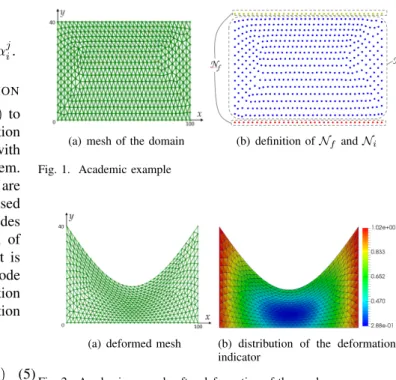
In order to illustrate the mesh deformation based on the RBF interpolation method, a simple academic example is used. The 2D spatial domain is rectangular shape discretized by triangle elements (fig. 1). The two sets of node Nf and Ni are introduced to perform the deformation (Fig.1.b). The
displacement of the nodes ofNf is imposed according to their
x coordinates. Then, for a node nk ∈ Nf, the displacement
along the axis y is imposed such as
dy=
(
0 if y= 0
−25cos(π/100x) if y= 40 (6)
The displacements of the nodes of Ni are interpolated with
Gaussian functions for the RBF. Figure 2.a presents the deformed mesh. As the displacement of a node is calculated independently from the other ones, it is necessary to verify the conformity of the deformed mesh. Then, we propose an indicator based on the comparison of the determinant of the initial and the deformed element. Thus, the indicator is
de = dete−def/dete−init with dete−def and dete−init the
determinants of the deformed and initial element e. If the
indicator is positive for all elements, the deformation of the mesh is correct. If an element is shifted between both meshes and overlaps others elements, its indicator is negative and the deformed mesh is not conformal. The distribution of the indicator is presented in Fig. 2.b, it gives information of the deformation for all elements of the mesh.
(a) mesh of the domain (b) definition ofNf andNi Fig. 1. Academic example
(a) deformed mesh (b) distribution of the deformation indicator
Fig. 2. Academic example after deformation of the mesh
IV. NUMERICAL EXPERIMENT A. Presentation of the example
We consider a 2D magnetostatic example composed with
118401st order triangle elements. The device is composed by a stranded inductor supplied by a current, a magnetic core and a magnetic plate. The vector potential formulation is used to solve the problem, the strong formulation is
curl 1
µcurlA
=J (7)
with µ the magnetic permeability, J the current density of the stranded inductor and A the unknown potential. The mesh deformation is imposed on the plate, the boundary of mesh deformation is specified in fig. 3. In figure 4, the red and green nodes correspond to those of Nf and the orange
nodes to those of Ni. The position of green nodes is fixed
and the displacement of red nodes is imposed. The RBF interpolation method is performed onto the orange nodes. A rotation movement of 20 degrees in the clockwise direction is imposed for the plate. At first, the aim is to study the influence of the parameters of the RBF interpolation method on the mesh deformation. In a second time, local quantities are studied.
B. Influence of the iteration number
The RBF interpolation method can be applied iteratively. At each iteration, the method to calculate the new coordi-nates of the nodes is performed with the intermediate mesh
Fig. 3. Magnetostatic problem
Fig. 4. Definition ofNf andNi
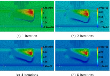
computed at the previous iteration. Then, a large deformation is decomposed in several smaller ones. Figure 5 presents the distribution of the deformation indicator for the last mesh after 1, 2, 4 and 8 iterations. Gaussian functions witha= 1is used for the RBF. For 1 and 2 iterations, the deformation indicator
(a) 1 iteration (b) 2 iterations
(c) 4 iterations (d) 8 iterations
Fig. 5. Influence of the iteration number on the mesh deformation with Gaussian functions anda= 1
is negative for several elements, the mesh is not conformal in this case. With 4 and 8 iterations, the final meshes are close and conformal. Then, an iterative approach of the RBF interpolation method increases the robustness of the mesh deformation.
C. Influence of the choice of RBF
We compare the mesh deformation for three different RBF with 4 iterations. Gaussian, multiquadric and inverse quadric functions are considered with the same value for the parameter
a (a= 1). Figures 6 and 5.c present the distributions of the deformation indicator for multiquadric and inverse quadric functions and for Gaussian functions respectively. For all
(a) multiquadric (b) inverse quadric Fig. 6. Influence of the radial basis function on the mesh deformation
cases, the final mesh is conformal. The influence of functions is not very significant on our example. Nevertheless, we can observe that the mesh deformation is smoother with the inverse quadric function than with the two others.
D. Influence of the parameter a
The parameter a of functions presented in table I enables to adjust the domain of influence of nodes with imposed displacements on a node to be moved. Greaterais important, most influential is the displacement of node by nodes with a fixed displacement. Figures 7 and 5.c present the distributions of the deformation indicator for Gaussian functions with
a= 0.5 and1.5for 4 iterations.
(a)a= 0.5 (b)a= 1.5
Fig. 7. Influence of the parameteraon the mesh deformation
E. Influence on local quantities
Figure 8 presents the distributions of the magnetic flux density. Gaussian and inverse quadric functions are applied for the RBF interpolation. The influence of the choice RBF is not so significant. In fact, the difference of the maximal magnitude is0.2mT.
(a) with Gassian functions and
a= 1
(b) with inverse quadric functions anda= 2
Fig. 8. Distribution of the magnetic flux density (T) for a rotation movement of the plate
V. APPLICATION
A 3D application example based on a NDT device is consid-ered (Fig. 9) [6]. This consists in a stranded inductor supplied by a sinusoidal current, a magnetic core and a conductive plate with a crack. The electric formulation is used to solve the problem in the time domain, the strong formulation is
curl 1
µcurlA
+σ(∂tA+gradϕ) =J (8)
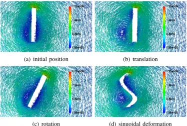
with σ the electric conductivity of the plate and ϕ the scalar electric potential defined within the plate. The mesh is composed of 203659 1st order tetrahedra. The aim is to study the difference of magnetic flux with and without crack. From the original mesh with an initial shape of the crack, the RBF interpolation method is performed to modify the geometry of the default. Inverse quadric functions are used for the RBF with 8 iterations to reach the final deformation (see IV-B). Figure 10 presents the distribution of the deformation indicator for a translation, a rotation and a sinusoidal deformation of the crack. For all cases, the deformed mesh is conformal. Figure
(a) 3D view (b) 2D view
Fig. 9. Mesh of the NDT example
(a) translation (b) rotation
(c) sinusoidal deformation
Fig. 10. Deformation indicator for three different deformations
11 presents the distribution of the eddy current density for the different shapes of the crack. Figure 12 presents the evolution of the difference of the magnetic flux flowing through the stranded inductor for different shapes of the crack. For the initial position and for a rotation of the crack, the evolution are close. The maximal magnitude is obtained with the crack translated from the initial position. In term of computational time, the mesh deformation required about 8.5s for 5576 nodes to be moved. This is inferior to the computational time necessary to solve one time step of the problem (10s).
(a) initial position (b) translation
(c) rotation (d) sinuoidal deformation Fig. 11. Distribution of the eddy current density for the different shapes of the crack
Fig. 12. Difference of the magnetic flux associated with the inductor
VI. CONCLUSION
The RBF interpolation method has been developed with low frequency electromagnetic problem solved by the FE method. A 2D academic magnetostatic example has been used to study the influence of the parameters of the RBF interpolation. A deformation indicator has been introduced to verify the validity of the deformed mesh. Then, a 3D magnetodynamic problem based on a NDT device has been studied. Different shapes of the crack have been obtained from the deformation of the initial geometry of the default. From the studied examples, the RBF interpolation method seems to be an interesting approach for the deformation of the shape of electromagnetic device.
REFERENCES
[1] L. Piegl, W. Tiller, The NURBS book, Springer 1997
[2] M.D., Buhmann, Radial Basis Functions, Cambridge University Press, 2003.
[3] Z. Bontinck, J. Corno, P. Bhat, H. De Gersem, S. Sch¨ops Modelling of a Permanent Magnet Synchronous Machine Using Isogeometric Analysis,
Computational Engineering, Finance, and Science, 2017.
[4] C. Willberg U. Gabbert, ”Development of a three-dimensional piezo-electric isogeometric finite element for smart structure applications, Acta Mechanica., vol. 223, pp. 1837-1850, 2012.
[5] A. de Boer, M.S. van der Schoot, H. Bijl, Mesh deformation based on radial basis function interpolation, Conference on Computational Fluid and Solid Mechanics, vol. 85, pp. 784-795, 2007.
[6] T. Henneron, Y. Le Menach,F. Piriou, O. Moreau, S. Clenet, J-C. Ducreux and J-C Verite, Source Field Computation in NDT Applications, IEEE. trans. mag., vol. 43, no. 4, pp. 1785-1788, 2007.