Bayesian model calibration with interpolating polynomials based on adaptively weighted Leja nodes

Bayesian Model Calibration with Interpolating

Polynomials based on Adaptively Weighted Leja Nodes

1_{Centrum Wiskunde & Informatica, P.O. Box 94079, 1090 GB, Amsterdam,} The Netherlands.

2_{Delft University of Technology, P.O. Box 5, 2600 AA, Delft, The Netherlands.} Received 27 August 2018; Accepted (in revised version) 17 May 2019

Abstract. An efficient algorithm is proposed for Bayesian model calibration, which is commonly used to estimate the model parameters of non-linear, computationally expensive models using measurement data. The approach is based on Bayesian stat-istics: using a prior distribution and a likelihood, the posterior distribution is ob-tained through application of Bayes’ law. Our novel algorithm to accurately determine this posterior requires significantly fewer discrete model evaluations than traditional Monte Carlo methods. The key idea is to replace the expensive model by an inter-polating surrogate model and to construct the interinter-polating nodal set maximizing the accuracy of the posterior. To determine such a nodal set an extension to weighted Leja nodes is introduced, based on a new weighting function. We prove that the con-vergence of the posterior has the same rate as the concon-vergence of the model. If the convergence of the posterior is measured in the Kullback–Leibler divergence, the rate doubles. The algorithm and its theoretical properties are verified in three different test cases: analytical cases that confirm the correctness of the theoretical findings, Burgers’ equation to show its applicability in implicit problems, and finally the calibration of the closure parameters of a turbulence model to show the effectiveness for computa-tionally expensive problems.

AMS subject classifications: 62F15, 65D0

Key words: Bayesian model calibration, interpolation, Leja nodes, surrogate modeling.

1

Introduction

Estimating model parameters from measurements is a problem of frequent occurrence in many fields of engineering and many different approaches exist to solve this prob-∗_{Corresponding author.Email addresses:[email protected](L.M.M. van den Bos),}

[email protected](B. Sanderse),[email protected](W.A.A.M. Bierbooms), [email protected](G.J.W. van Bussel)

lem. We consider non-linear calibration problems (or inverse problems) where a forward evaluation of the model is computationally expensive. The approach we follow is of a stochastic nature: the unknown parameters are modeled using probability distributions and information about these parameters is inferred using Bayesian statistics. This ap-proach is often calledBayesian model calibration.

Bayesian model calibration [19, 32, 33] is a systematic way to calibrate the paramet-ers of a computational model. By means of a statistical model to describe the relation between the model and the data, the calibrated parameters are obtained in the form of a random variable (called theposterior) by means of Bayes’ law. These random variables can then be used to assess the uncertainty in the model and to make future predictions. This procedure is well-known in the field of Bayesian statistics, where the goal is to infer unmeasured quantities from data. The calibration approach has already been applied many times, for example to calibrate the closure parameters of turbulence models [7, 11]. A similar example is considered in this work.

Possibly the largest drawback of Bayesian model calibration is the expensive sampling procedure that is necessary. Because the posterior depends to a large extent on the model, which is only known implicitly (e.g. a computer code numerically solving a partial differ-ential equation), determining a sample from the posterior is mostly done using Markov chain Monte Carlo (MCMC) methods [14, 25], requiring many expensive model eval-uations. Improvements have been made to accelerate these MCMC methods, e.g. the DREAM algorithm [39] or adaptive sampling [42]. Replacing the sampling procedure itself is also possible, e.g. methods based on sparse grids [6, 22] or Approximate Bayesian Computation [2, 9, 20]. However, this encompasses stringent assumptions on the statist-ical model or still requires many model runs as the shape of the posterior is unknown.

A different approach is followed in the current article. In essence we are follow-ing the approach of Marzouk et al. [24], which has been used several times in literat-ure [1, 4, 23, 28, 31, 44–46]. The key idea in our procedliterat-ure is to replace the model in the calibration step with asurrogate(orresponse surface) that approximates the computation-ally expensive model. MCMC can then be used to sample the resulting posterior without a large computational overhead.

Various approaches to construct this surrogate in a Bayesian context exist, for example Gaussian process emulators [36] or non-intrusive polynomial approximations [43]. In this work the latter is considered, because polynomial approximations provide high order (up to exponential) convergence for sufficiently smooth functions. Contrary to the commonly used pseudo-spectral projection methods, which are commonly known as generalized Polynomial Chaos Expansions, we choose to use interpolation of the computationally expensive model. The reason for this is that the error of a polynomial interpolant is usu-ally measured using the absolute error (theL∞norm), contrary to the mean squared error (theL2norm) that is used for the pseudo-spectral approaches. As the model is used as in-put in the Bayesian analysis, having absolute error bounds on the surrogate significantly simplifies the analysis. Moreover, the convergence of a pseudo-spectral expansion deteri-orates significantly if the surrogate is not constructed using the statistical model [21]. This

happens in particular if the expansion is constructed with respect to the prior (which is the usual approach) and the likelihood contains significant information (i.e. their relative entropy is high).

The interpolating surrogate model is built using Leja nodes. Probability density func-tions can be incorporated using weighted Leja nodes [18, 26]. We extend weighted Leja nodes to adaptively refine the interpolating polynomial by using obtained posterior in-formation. As extensive theory about interpolation polynomials exists (e.g. [16]), we can prove convergence of the estimated posterior with mild assumptions on the likelihood. This extends previous work [4, 24], in which the likelihood is assumed to be Gaussian. The end result is an interpolating polynomial that can be used in conjunction with the likelihood and the prior to obtain statistics of the posterior.

To demonstrate the applicability of our methodology, we will employ three differ-ent classes of test problems. The first class consist of functions that are known explicitly and can be evaluated fast and accurately. We will use these to show the effectiveness of our nodal set compared to commonly used methods. The second class consists of prob-lems that are defined implicitly, but do not require significant computational power to solve. For this, we employ the one-dimensional Burgers’ equation. In this case, it is pos-sible to compare the estimated posterior with a posterior determined using Monte Carlo methods. The last class consists of problems of such large complexity that a quantitative comparison with a true posterior is not possible anymore. As example we consider the calibration of closure coefficients of the Spalart–Allmaras turbulence model.

This paper is set up as follows. First, we discuss Bayesian model calibration and in-troduce the adaptively weighted Leja nodes. In Section 3 the theoretical properties of the algorithm are studied and its convergence is assessed. Section 4 contains numerical tests that show evidence of the theoretical findings and in Section 5 conclusions are drawn.

2

Bayesian model calibration with a surrogate

The focus is on the stochastic calibration of computationally expensive (possibly impli-citly defined) models. We denote this model byu:Ω→R_{, with}Ω⊂Rd _{(d=1,2,...). In}

this work we will not focus on the specific construction of this model, but for exampleu arises as a solution of a set of partial differential equations. Without loss of generality, we assume thatuis a scalar quantity. udepends ondparameters, which we will denote as vectorϑ= (ϑ1,...,ϑd)T∈Ω. One can think ofϑas parameters inherent to the model, such

as fitting parameters or other closure parameters.

The goal of Bayesian model calibration is to infer knowledge about the model para-meters, given measurement data of the process modeled by u. To this end, we assume that a vector of measurements z= (z1,...,zn)T is given, with zk∈R. This data can be

provided by various means, for example by measurements or by the results of a high-fidelity model. Using parametersϑ, a statistical model is formulated describing a relation between the modelu(ϑ)and the datazby means of random variables that model among

others discrepancy, error, and uncertainty. For example, these random variables account for measurement errors and numerical tolerances. Using Bayesian statistics [12], the pos-terior of the parameters is formulated by means of a probability density function (PDF).

Throughout this article we letp(ϑ)be the prior, a PDF containing all prior information ofϑ obtained through physical constraints, assumptions, or previous experiments. The likelihoodp(z|ϑ)is obtained through the statistical relation between the modeluand the dataz. Possibly the most straightforward example iszk=u(ϑ)+εk, whereε= (ε1,...,εn)T

is assumed to be multivariate Gaussian distributed with mean0and covariance matrix

Σ_{. This yields the following likelihood:}

p(z|ϑ)∝exp −1 2d T_Σ−1_d

, withda vector such thatdk=zk−u(ϑ). (2.1) dis the so-called misfit. Bayes’ law is applied to obtain the posteriorp(ϑ|z), i.e.

p(ϑ|z)∝_p(z|ϑ)p(ϑ). (2.2) The posterior PDF can be used to assess information about the parameters of the model, e.g. by determining the expectation or the MAP estimate (i.e. the maximum of the pos-terior). The uncertainty of these parameters can be quantified by determining the mo-ments of the posterior PDF.

Note that the posterior depends on the likelihood, which requires an expensive eval-uation of the model (see (2.1)). Therefore sampling the posterior through the application of MCMC methods [14, 25] is typically intractable for such models.

Vector-valued modelsucan be incorporated in this framework straightforwardly, al-though the likelihood requires minor modifications. Typically an observation operator is introduced that restrictsuto the locations where measurement data is available. We will discuss an example of this in Section 4.3.

Throughout this article we assume the likelihood is a continuously differentiable, Lipschitz continuous function of the misfit d or (more general) of the model u. This is true for the multivariate Gaussian likelihood and (more general) for any likelihood which has additive errors (see [19] for more examples in the context of Bayesian model calibration). There are no further constraints on the structure of the likelihood and the prior in this work, but we do not incorporate the calibration ofhyperparameters, i.e. para-meters introduced solely in the statistical model (an example would be the calibration of the standard deviation ofε). Moreover, we assume the prior is not improper, i.e. it is a well-defined distribution withRΩp(ϑ)dϑ=1. Even though this prohibits the usage of a

uniform prior on an unbounded interval, in practice our methods can be applied in such a setting.

The outline of the proposed calibration procedure is as follows. LetuN be an

inter-polating surrogate of u using N distinct nodes and model evaluations. Using uN, an

estimated posterior can be determined, which is used to obtain the(N+1)th _{node. The}

resulting posterior, because the computationally expensive model is replaced with an explicitly known surrogate.

First, we briefly introduce the interpolation polynomial for sake of completeness. Then the nodal set we will use, the Leja nodes, will be introduced.

2.1 Interpolation methods

In general an interpolating polynomial can be defined as follows. Letu:Ω→R_withΩ⊂ Rd_{be a continuous function. LetDbe given and define the set}P_{(N,d)(withN=(}d+D

D )) to

be alld-variate polynomials of degreeDand lower. Using a nodal setXN+1={x0,...,xN}

and evaluations of u at each node (i.e. u(xk) for k=0,...,N) the goal is to determine a

polynomialuN∈P(N,d)such that

uN(xk) =u(xk), fork=0,...,N. (2.3)

This construction can be extended to anyN=1,2,3,..., provided that the monomials of the spaceP_{(N,d)form a well-ordered set. Throughout this article, we use a graded reverse}

lexicographic order.

2.1.1 Univariate interpolation

In the case ofd=1, it is well-known that if all nodes are distinct the interpolation poly-nomial can be stated explicitly using Lagrange interpolating polypoly-nomials, i.e.

uN(x) = (LNu)(x):= N

∑

∏

HereLN is a linear operator that yields a polynomial of degreeN, which we will denote

asuN. By construction, the Lagrange basis polynomialsℓ_kNhave the propertyℓN_k (xj)=δk,j

(i.e.ℓN

k (xj) =1 ifj=kandℓNk (xj) =0 otherwise). ThereforeuN(xk) =u(xk)for allk, such

that it is indeed an interpolating polynomial.

The barycentric notation [3] can be used to numerically evaluate the interpolation polynomial given a nodal set (which is unconditionally stable [15]).

2.1.2 Multivariate interpolation

The Lagrange interpolating polynomials can be formulated in a multivariate setting, by defining them in terms of the determinant of a Vandermonde-matrix:

uN(x) = (LNu)(x):= N

∑

whereV(x0,...,xN)is the(N+1)×(N+1)Vandermonde-matrix with respect to the nodal

set{x0,...,xN}, i.e.

Vi,j(x0,...,xN) =x αj

Here,αj∈Nd are defined such that for α= (α1,...,αd)andx= (x1,...,xd), we have xα=

xα1

1 ···x αd

d . As stated before,αjare sorted using the graded reverse lexicographic order (i.e.

first compare the total degree, then apply reverse lexicographic order to equal monomi-als). This implies thatkαjk1is a sorted sequence inj. Multivariate interpolation by means

of this Vandermonde-matrix is only well-defined ifVis non-singular (thenXN+1is called

a poised interpolation sequence with respect toP_{(N,d)). All nodal sequences constructed}

in this article are (by construction) poised.

There exist various other monomial orders, for example for the purpose to construct a sparse grid [27]. Also adaptive choices have been studied [26]. Often these approaches leverage structure in the underlying distribution by decomposing it indunivariate dis-tributions (i.e. the distribution is “tensorized”). Such efficient approaches cannot be ap-plied to the context of this article, because it is rarely the case that the posterior can be decomposed ind univariate distributions, due to the asymmetry in the model and the measurement data. Nonetheless, the framework and algorithms proposed in this work can easily accommodate different monomial orders.

Evaluating a multivariate interpolating polynomial numerically can be done in vari-ous ways. A commonly used approach is to rewrite (2.6) as

Vi,j(x0,...,xN) =ϕj(xi), (2.7)

whereϕj(x)are orthogonal basis polynomials (e.g. Chebyshev or Legendre polynomials).

The polynomialsϕjform a linear combination of monomials, so mathematically speaking

both approaches yield the same solution.

The nodal sets used in this article use the determinant of the Vandermonde-matrix. Therefore we use a QR factorization [13] of the Vandermonde-matrix to determine the interpolating polynomial and reuse the QR factorization to determine the nodal set (see Section 2.2 for details).

2.2 Weighted Leja nodes

For the purpose of Bayesian model calibration, we desire an algorithm to determine a nodal setXN for anyNhaving the following properties:

1. Accuracy: the nodal sets should yield an accurate posterior. We are mainly inter-ested in estimating the posterior, i.e. it is not strictly necessary to have an accurate surrogate model on the full domain.

2. Nested:we requireXi⊂Xjfori<j, such that the obtained interpolant can be refined

by reusing existing model evaluations.

3. Weighting: the goal is to determine the next node based on the posterior obtained so far. The algorithm of the nodal set should allow for this.

In this work we consider weighted Leja nodes, which form a sequence of nodes. The sequence is therefore by definition nested. First, we will define the univariate Leja nodes and generalize those to multivariate Leja nodes.

The definition of weighted Leja nodes is by induction. Letρ:R_→R_{+be a bounded}

PDF (withR_{+:= [0,}∞)) and let{x0,...,xN}be a sequence of Leja nodes. Then the next

node is defined by maximizing the numerator ofℓN+1

N+1(x), i.e.

xN+1:=argmax x∈R

ρ(x)|x−x0||x−x1|··· |x−xN|. (2.8)

This maximization problem does not necessarily have a unique solution. To ensure that a solution exists, it is necessary to assume that eitherρ(x)has bounded and closed support or (more generally) that the polynomials are dense in the space equipped with the ∞ -norm weighted with ρ(x), i.e. the norm kfkρ=kfρk∞=sup_x∈R|f(x)ρ(x)| [26]. Note

that the former implies the latter and thatρ has finite moments in these cases. If there are multiple values maximizing (2.8), we pick the one with smallest x to ensure that the sequence is reproducible (in multivariate spaces, we select the smallest one using a lexicographic ordering). The initial nodex0is defined as the smallest global maximum of

ρ(x).

If ρ(x) has finite moments, it decays faster than any polynomial grows for x→∞

(which makes the maximization problem above well-defined). To see this, assumeρ(x) decays slower than the polynomialxk_{grows fork>1, or equivalently assumeρ(x)>1/x}k

forx>_{A. Then Z} ∞ A x k_ρ(x)dx>Z ∞ A x k 1 xkdx=∞, (2.9)

which cannot be the case asρ(x)has finite moments. Notice that definition (2.8) can be rewritten as follows:

xN+1= argmax x∈R,ρ(x)>₀ logρ(x)+ N

∑

Ifρ(x)is bounded from below and above, i.e. A≤ρ(x)≤B for 0<_A<_Bandρ(x)has bounded support, the sum log|x−x0|+...+log|x−xN|will dominate the maximal value

for large N. Hence for anyx the value of the sum will increase (but remains bounded asρ(x)has bounded support) andρ(x)will remain constant (asρis independent of N). This implies that forρ(x)that are bounded from below and above, the influence of the weighting function decreases asNincreases.

Unweighted Leja nodes are defined with the uniform weighting function on [−1,1]. We want to emphasize that multiplying the weighting function with a constant yields an identical sequence. This property is very useful for our purposes, as it allows us to neglect the constant of proportionality (often called the evidence) in Bayes’ law (see (2.2)). Examples of these sequences are depicted in Fig. 1. Throughout this article, univari-ate Leja nodes are determined by applying Newton’s method to the derivative of the

−1−0.5 0 0.5 1 X

N

(a) Uniform (“unweighted”)

−1−0.5 0 0.5 1 X N (b) Beta (α=β=4) −4 −2 0 2 4 X N (c) Standard normal

Figure 1: Univariate Leja sequences for various number of nodes and various well-known distributions.

logarithm of the maximization problem above, i.e. (2.10) is solved instead of (2.8). By determining all local maxima between two consecutive nodes in parallel, large numbers of nodes can be calculated fast and accurately (as the maximization function is smooth between two nodes). Numerical cancellation is kept minimal by using extended precision arithmetic (with machine epsilon approximately 10−19).

The definition of univariate Leja nodes can be generalized to a multidimensional setting in a similar way as we did in Section 2.1.2 with interpolation. To this end, let ρ:Rd_→R_{+ be a multivariate PDF. Letx0∈}Rd _{be an initial node with ρ(x0)}>_{0. Then} given the nodesx0,...,xN, the next nodexN+1is defined as follows:

xN+1:=argmax

x∈Rd

ρ(x)|detV(x0,...,xN,x)|. (2.11)

Here,Vis the Vandermonmatrix defined in Section 2.1.2. The absolute value of the de-terminant ofVis independent of the set of polynomials that is used to constructV, so the definition is mathematically the same for both monomials and orthogonal polynomials.

Determining multivariate Leja nodes is less trivial compared to univariate nodes and is typically done by randomly (or quasi-randomly) sampling the space of interest and selecting the node that results in the highest determinant. It is significantly more com-plicated to reliably apply Newton’s method in this case, as the space cannot be easily partioned in regions where the local maxima reside. To reach a comparable accuracy, it is important to be able to use a large number of samples, so it must be possible to calculate the determinant fast. We suggest to calculate the determinant by an extended QR factor-ization of the(N+2)×(N+1)-matrixV(x0,...,xN)and to add the column containingxby

applying a rank-1 update. If a QR factorization has been calculated to determine the in-terpolating polynomial (see Section 2.1.2), it can be reused here. As a rank-1 update is an efficient procedure, a large number of samples can be used and therefore we assume that the approximation error is negligible in this case. Examples of Leja sequences defined by (2.11) can be found in Fig. 2.

−1 −0.5 0 0.5 1 −1 −0.5 0 0.5 1 X1 X2

(a) Uniform (“unweighted”)

−1 −0.5 0 0.5 1 −1 −0.5 0 0.5 1 X1 X2 (b) Multivariate Beta (α=β=4) −2 −1 0 1 2 −2 −1 0 1 2 X1 X2 (c) Multivariate normal

Figure 2: Multivariate Leja sequences of 25 nodes using various well-known distributions.

2.3 Calibration using Leja nodes

In this section we will derive a weighting function to be used in the interpolation proced-ure discussed in the previous section, with the goal to approximate the posterior. Theoret-ical details are provided in Section 3. First we discuss the rationale behind the weighting function in Section 2.3.1. The weighting function itself is presented in Section 2.3.2 and the mathematical derivation it is based upon is presented in Section 2.3.3. The weighting function has one free parameter, which is discussed in more detail in Section 2.3.4. 2.3.1 Rationale

If the posterior is known explicitly and samples can be readily drawn from it, it is possible to determine weighted Leja nodes with weighting functionρ(ϑ) =p(ϑ|z). These nodes provide an interpolant that is very suitable for evaluating integrals with respect to the posterior (this is commonly known as Bayesian prediction). However, the posterior is generally not explicitly available because it depends on the model u, which in itself is not known explicitly and can only be determined on (finitely many) nodes. Therefore the need arises for an interpolation sequence that approximatesusuch that the posterior determined with this approximation is accurate.

To this end, let pN(ϑ|z)be the posterior determined usinguN(ϑ), i.e. the interpolant

ofuusingN+1 nodes inϑ. If the likelihood is according to (2.1),pN is as follows:

pN(ϑ|z)∝p(ϑ)exp −1 2d T_Σ−1_d

, withda vector such thatdk=zk−uN(ϑ). (2.12)

We will use the definition of the weighted Leja nodes from (2.11) to determine the next node. The natural idea is to construct pN+1(ϑ|z)(i.e. a new approximation of the

pos-terior) by determining a new weighted Leja node usingpN(ϑ|z)(i.e. the existing

approx-imation of the posterior). Such a sequence can be numerically unstable, because it solely places nodes in regions where the approximate posterior is high and therefore yields spurious oscillations in other regions in the domain.

The key idea is to balance between the accuracy of the interpolant and the accuracy of the posterior. There are various methods to do this, but we choose to temper the effect of the (possibly inaccurate) approximate posterior by adding a constant valueζto it. The higher thisζ, the more the posterior tends to the prior. In Section 3.2 it is demonstrated that for anyζ>_{0, the interpolant constructed with these weighted Leja nodes has (at least)} the same asymptotic convergence rate as an interpolant determined with weighted Leja nodes without adaptivity. Ifζ is chosen correctly, the approximate posterior is already accurate for moderately smallN.

2.3.2 The adaptive weighting function

To introduce this construction formally, we assume that a functionP:R_→R_{+exists such}

that

p(z|ϑ) =P(u(ϑ)), (2.13) where P typically is a PDF which follows from the statistical model. In the example discussed in (2.1)Pis a Gaussian PDF, i.e.

P:R_→R_{+, withP(u)}∝_exp −1 2d T_Σ−1_d and dk=zk−u. (2.14)

We assume that the functionPis globally Lipschitz continuous and continuously dif-ferentiable. Many statistical models used in a statistical setting yield Lipschitz continu-ousP, because a bounded continuously differentiable functionP(u)with P′(u)→0 for u→ ±∞_{is Lipschitz continuous. The domain of definition ofPis the image of the model}

u(ϑ), so functionsPthat are only Lipschitz continuous in the set described by the image ofu(ϑ)also fit in this framework (for example the Gamma distribution on the positive real axis).

The weighting function proposed in this article, calledqN, clearly depends onN:

qN(ϑ|z) =|P′(uN(ϑ))|p(ϑ)+ζp(ϑ), whereζ>0 is a free parameter. (2.15)

So, ifϑ0,...,ϑNare the firstN+1 Leja nodes,ϑN+1is determined as follows: ϑN+1=argmax

ϑ

qN(ϑ|z)|detV(ϑ0,...,ϑN,ϑ)|. (2.16)

Here the derivativeP′is with respect tou, i.e. P′(u(ϑ)) =∂P

∂u(u(ϑ)). (2.17)

We want to emphasize that for the evaluation ofP′(uN(ϑ))no costly evaluation of the full

modeluis necessary, sinceP′ is independent ofu. In the example from (2.1),P′becomes the following: P′:R_→R_{, with P}′_(u)∝−1 2 1TΣ−1d+dTΣ−11exp −1 2d T_Σ−1_d and dk=zk−u, with1= (1,1,...,1)T∈Rn_.

2.3.3 Mean value theorem

The weighting functionqN as defined in (2.15) follows naturally by applying the mean

value theorem to the error of the approximate posterior. This introduces the derivativeP′ in the expression. To this end, let a fixedϑbe given, and apply the mean value theorem as follows:

|pN(ϑ|z)−p(ϑ|z)|=|P(uN(ϑ))−P(u(ϑ))|p(ϑ) =|P′(ξ)||uN(ϑ)−u(ϑ)|p(ϑ)

=|P′(uN(ϑ))+ζϑ||uN(ϑ)−u(ϑ)|p(ϑ), (2.18)

withξ an (unknown) value betweenuN(ϑ)andu(ϑ)andζϑ=P′(ξ)−P′(uN(ϑ)).

Essen-tiallyζϑ is used to represent higher order derivatives ofPin this expression. The value of ζϑ depends on ϑ and on the modelu, which is not explicitly known. By further ex-pandingP′, it can be shown thatζϑ scales with|uN(ϑ)−u(ϑ)|, provided thatP is twice

differentiable with bounded second order derivative: ζϑ=P′(ξ)−P′(uN(ϑ))

=1 2P

′′_{(ξ)(b u}

N(ϑ)−u(ϑ)), for aξbbetweenP′(uN(ϑ))andP′(u(ϑ)).

Hence ifuN(ϑ)→u(ϑ) for N→∞ and P′′ bounded (or: the divided difference of P′ is

bounded), it holds thatζϑ→0 forN→∞_{. In this work, the constantζϑis used to measure}

how far the likelihood of the interpolant is from the likelihood of the true model. The idea is to add a Leja nodeϑN+1where the error in the posterior is large, though such that

the interpolant remains stable. The weighting functionqN as introduced before follows

by taking the∞_{-norm in}ϑon both sides of (2.18):

kpN(ϑ|z)−p(ϑ|z)k∞=kP(uN(ϑ))−P(u(ϑ))k∞

=k|P′(ξ)|(uN(ϑ)−u(ϑ))p(ϑ)k∞

≤ k |P′(uN(ϑ))|+ζ uN(ϑ)−u(ϑ)p(ϑ)k∞

=k(uN(ϑ)−u(ϑ))qN(ϑ)k∞, (2.19)

withζ≥ |ζϑ|=|P′(ξ)−P′(uN(ϑ))|for allϑ.

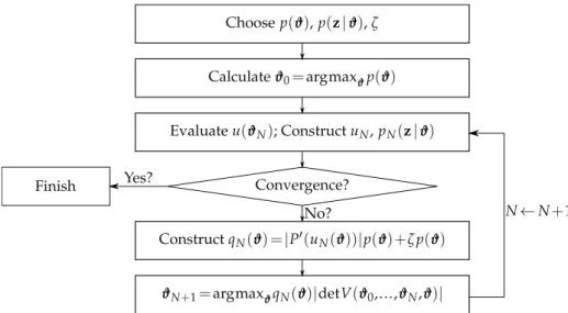
The algorithm proposed in this article is to (iteratively) firstly determineqN, secondly

determine ϑN+1 using (2.16), and finally determineu(ϑN+1) and reconstruct the

inter-polant (which yieldsuN+1and consequently pN+1(ϑ|z)). This algorithm is sketched in

Fig. 3. Convergence can be assessed in various ways, for example using the∞-norm or the Kullback–Leibler divergence. We will use the∞_{-norm, as determining the Kullback–}

Leibler divergence in higher-dimensional spaces is numerically challenging.

The exact value ofζϑ is not known a priori and depends onϑ. Nonetheless, we will demonstrate that for anyζ>_{0 it holds that ku−uNk∞→0 (for N→}∞_{), provided that}

“conventional” weighted Leja nodes produce a converging interpolant. If uN→u for

N→∞_{, the exact value of}ζconverges to 0, hence any value ofζwill work for sufficiently largeN. We will further study the convergence of this method in Section 3.

Choosep(ϑ_),p(z|ϑ),ζ Calculateϑ_0=argmax ϑp(ϑ) Evaluateu(ϑ_N); ConstructuN,pN(z|ϑ) ϑ_N+1=argmaxϑqN(ϑ)|detV(ϑ0,...,ϑN,ϑ)| Convergence? Finish Yes? No? N←N+1 ConstructqN(ϑ) =|P′(uN(ϑ))|p(ϑ)+ζp(ϑ)

Figure 3: Schematic overview of the algorithm proposed in this article.

2.3.4 Choice ofζ

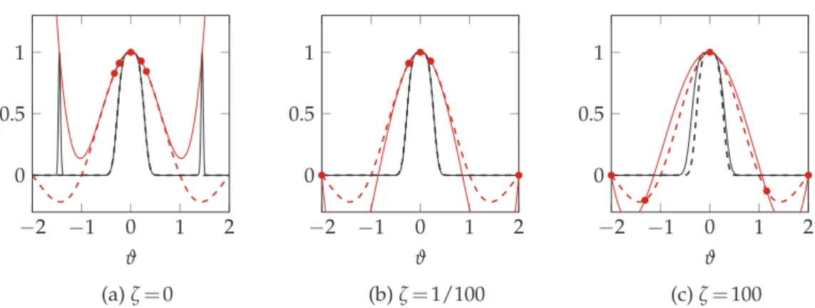
To illustrate the behavior of weighting function (2.15), examples of interpolants obtained using Leja nodes weighted usingqN in conjunction with the exact posterior are depicted

in Fig. 4. Here the parameterϑ of the univariate function u(ϑ) =sinc(ϑ) =sin(ϑ)/ϑ is “calibrated” using the Gaussian likelihood from (2.14) withσ=1/10, a uniform prior defined on[−2,2], and one data point atz1=1. Hence the exact posterior is as follows:

p(ϑ|z1)∝ ( exp− 1 2σ2|u(ϑ)−z1|2 , if|ϑ| ≤2, 0, otherwise. (2.20)

The weighting function under consideration is qN(ϑ) =|P′(u(ϑ))|+ζ, whereu is used

instead ofuNto illustrate the effect ofζ.

If ζ=0 (no tempering) the interpolant is indeed accurate with respect to the pos-terior (i.e. the weighted p(ϑ|z1)-norm), but yields an incorrect approximate posterior

because the interpolant crosses the value of the data incorrectly aroundϑ=±1.5. These spurious oscillations disappear for larger N, but for different test cases this is not ne-cessarily the case (as it requires global analyticity). Forζ =100, it is guaranteed that ζ≥ |P′(ξ)−P′(uN(ϑ))|for allϑ, but the nodes determined with that value are, due to the

large variations in the determinant of the Vandermonde-matrix, not sensitive to small variations in the approximate posterior, and are therefore pointwise close to unweighted Leja nodes (e.g. compare Fig. 4c with Fig. 1a). The best strategy is to take a small non-zero value ofζ, which balances posterior accuracy with stability. For such a small non-zero value, the second and third node are basically unweighted Leja nodes (and end up on the boundary). This does demonstrate the importance of tempering on the effect of the

ap-−2 −1 0 1 2 0 0.5 1 ϑ (a)ζ=0 −2 −1 0 1 2 0 0.5 1 ϑ (b)ζ=1/100 −2 −1 0 1 2 0 0.5 1 ϑ (c)ζ=100

Figure 4: Interpolation of thesinc function using 5 weighted Leja nodes with respect to the posterior using a tempering parameter ζ. The model u(ϑ) and (unscaled) posterior p(ϑ|z1) are depicted in red and black

respectively. The solid line represents the result constructed by means of interpolation and the “true” model and posterior are depicted using a dashed line.

proximate posterior, which becomes especially important if the functionuis not globally analytic (but “only” continuous).

The key point in obtaining a converging interpolant is thatζ>_{0. Ifζ=0, the} inaccur-acy of uN can significantly deteriorate the convergence (see Fig. 4), except possibly ifu

is globally analytic. If the goal is to optimizeζ, we suggest a heuristically adaptive ap-proach. Start withζ=ζ0>0 and for each iteration, multiplyζwith a constantk>1 if the

error in the posterior increases and divideζbykif the interpolation error decreases. The error can be estimated by comparing two consecutive approximate posteriors. This pro-cedure is however not necessary to obtain convergence for the examples in this article, for which a fixed value ofζis sufficient.

3

Convergence of the posterior

In this section the convergence of the estimated posterior to the true posterior is studied, denoted as follows:

kpN(ϑ|z)−p(ϑ|z)k∞→0, forN→∞. (3.1)

It is difficult to theoretically demonstrate that this is case, since the convergence rate of interpolants constructed with Leja nodes is only known in some specific cases. How-ever, we will demonstrate that the convergence rate of an interpolant determined with adaptively weighted Leja nodes is similar to one determined with Leja nodes without ad-aptivity, such that all results on the convergence of these conventional Leja nodes carry over.

The analysis is split into two parts. First, in Sections 3.1 and 3.2 the focus is on the model, i.e. it is assessed in which caseskuN−ukp(ϑ)→0 for N→∞(where p(ϑ)denotes the prior). In Section 3.1 convergence properties of interpolation methods are briefly

reviewed. In Section 3.2 the focus is specifically on Leja nodes, a case that will be assessed numerically. Moreover, the close relation between adaptively weighted Leja nodes and Leja nodes without adaptivity is considered.

The second part of the analysis consists of demonstrating that the posterior converges if the interpolant converges. Specifically, in Section 3.3 the following is demonstrated:

kpN(ϑ|z)−p(ϑ|z)k∞≤DkuN−ukp(ϑ), withDa constant independent ofN. (3.2) The conventional way of describing the distance between two distributions is by means of the Kullback–Leibler divergence. In Section 3.4 it is proved that if the interpolant converges to the true model, the Kullback–Leibler divergence between the approximate posterior and the true posterior converges to zero. Moreover, the rate of convergence doubles.

3.1 Accuracy of interpolation methods

The accuracy of interpolation methods can be assessed in two ways: usingpointwiseerror bounds which are typically based on Taylor expansions andglobalerror bounds which are typically based on the Lebesgue inequality. We will use the latter type.

LetP_{(K) =}P_{(K,1), i.e. all univariate polynomials of degree less than or equal toK.}

We assumeu∈C[−1,1](i.e. a continuous function defined in[−1,1]) andkuk∞<∞if not

stated otherwise. It is well-known thatC[−1,1]equipped with the normk·k∞ forms a

Banach space.

Let XN={x0,...,xN} ⊂[−1,1]be a set of interpolation nodes and let LN:C[−1,1]→

P_{(N)be the Lagrange interpolation operator (see (2.4)) that determines the interpolating}

polynomial given the nodal setXN. Then for any polynomial ϕN of degreeNwe have kLNu−uk∞≤(1+kLNk∞)kϕN−uk∞, (3.3)

whereΛ_N:=kLNk∞=sup_x∈[−1,1]∑_kN₌₀|ℓ_kN(x)|is the operator norm ofLN induced by the

norm k·k∞ discussed above. ΛN is called the Lebesgue constant [16]. The inequality

holds for any polynomialϕN, so an immediate result is the Lebesgue inequality: kLNu−uk∞≤(1+ΛN) inf

ϕN∈P(N)

kϕN−uk∞. (3.4)

The obtained expression contains a part that solely depends on the nodes, i.e. (1+ Λ_N), and a part that solely depends on the function u, i.e. infϕN∈P(N)kϕN−uk∞. The

second part is commonly known as the best approximation error. In the procedure used for calibration, nodes are determined using a weighting functionρ. To assess the accuracy of nodes that use weighting, we reconsider the weighted∞_-normkukρ=kρuk∞. Here,

we assume thatρ:Ω→R_{+ is a bounded PDF}†_{, such that thatC(}Ω)equipped with the †_{The boundedness is not strictly necessary forC(Ω)to be a Banach space, but for the cases discussed in this}

normk·kρ forms a Banach space. The support ofu(sayΩ) is allowed to be unbounded,

in contrast to the unweighted case. The unweighted case is a special case of the weighted case.

Using this norm we can derive a similar estimate as (3.4) by introducing [18]:

Λρ_N:=kLNkρ=sup x∈R N

∑

Here, Λρ_{N is called the weighted Lebesgue constant, i.e. the norm of the operator u}→ ρLN(u/ρ). We call the result the weighted Lebesgue inequality:

kLNu−ukρ≤(1+Λρ_N) inf ϕN∈P(N)

kϕN−ukρ. (3.6)

The Lebesgue inequality does not readily provide means to estimate the order of con-vergence. For this purpose, Jackson’s inequality [17, 30] can be used, that relates the best approximation error to the modulus of continuity ofu. Important for this work is that if uis Lipschitz continuous (or continuous and bounded on a compact domain) then a sublinearly growing Lebesgue constant provides a converging interpolant. Various other results on this topic exist, the interested reader is referred to the accessible introduction in the book of Watson [40] and the references therein for more information.

3.2 Lebesgue constant of Leja nodes

It is both an advantage and a disadvantage that the Lebesgue constant solely depends on the nodal set: we do not have to take the model into account to estimate the accuracy, but the resulting estimate does not leverage any properties of the model. The algorithm discussed in Section 2.3 does use the model and therefore cannot be fit directly in the framework set out in the previous section.

Many nodal sets exist with a logarithmically growing Lebesgue constant, which is asymptotically the optimal growth. For example, Chebyshev nodes (i.e. the nodes from the Clenshaw–Curtis quadrature rule) have Λ_N=O(logN)[16]. Moreover, we already stated that the Chebyshev nodes are nested such that the nodes forN=2l+1 (for integer l) are contained in the nodes for N=2l+1+1. However, the Chebyshev nodes are only defined in an unweighted setting. Another well-known example are equidistant nodes, which have an exponentially growing Lebesgue constant. This can be observed by inter-polating Runge’s function.

Although it is known that the Lebesgue constant of both weighted and unweighted Leja sequences grows sub-exponentially [18, 37, 38], the exact growth (or a strict upper bound) is not known. We have therefore numerically determined the Lebesgue constant forNup to 30000 for several distributions and observedΛρ

N≤N, see Fig. 5. For the

pur-pose of these figures, the Leja nodes and the Lebesgue constant have been determined by applying Newton’s method to the derivative of the function, as described in Section 2.2.

100 102 104 100 102 104 N Λ ρ N (a) Uniform 100 102 104 100 102 104 N Λ ρ N (b) Standard Gaussian 100 102 104 100 102 104 N Λ ρ N (c) Beta (α=β=4)

Figure 5: The weighted Lebesgue constant of weighted Leja nodes for three different distributions. The solid line depictsΛ_N=N. 100 101 102 100 101 102 N Λ qN N (a)ζ=0 100 101 102 100 101 102 N Λ qN N (b)ζ=1/100 100 101 102 100 101 102 N Λ qN N (c)ζ=100

Figure 6: The weighted Lebesgue constant of adaptively weighted Leja nodes using a Gaussian likelihood with

σ=1/10, a uniform prior on[−2,2], a single data pointz1=1, and the functionu(ϑ) =sinc(ϑ). The solid line

depictsΛ_N=N.

Except for some specific cases (such as the unit disk [5]), not much is known about the Lebesgue constant in the multivariate case. Unfortunately, as far as the authors know, it is difficult to determine the Lebesgue constant of multivariate Leja nodes accurately enough to create a similar plot as Fig. 5. For small numbers of nodes (N.100) and low dimensionality (d.5) the Lebesgue constants seem to grow similarly, but the sampling procedure significantly deteriorates the accuracy. Moreover this number is too small to draw conclusions about general asymptotic behavior. Nonetheless, the numerically de-termined growth of the Lebesgue constant is sufficient for the purposes in the current article (as N.100 throughout this article). We want to emphasize that contrary to the Lebesgue constant, large numbers of multivariate Leja nodes can be determined effi-ciently by means of sampling, as evaluating the maximization function is significantly more straightforward (see Section 2.2).

These results do not carry over straightforwardly to the case of adaptively weighted Leja nodes where the weighting function depends on the number of nodes. However, for reasonably smallNthe Lebesgue constant can be assessed numerically. To this end, we have determined the Lebesgue constantΛqN

N , i.e. the Lebesgue constant weighted with

qNfrom (2.15), of adaptively weighted Leja nodes using the aforementioned example of a

Gaussian likelihood in conjunction with the functionu(ϑ) =sinc(ϑ)(see Fig. 6). Determ-ining Leja nodes in this case is still relatively straightforward, but determDeterm-ining the

Le-besgue constant accurately is significantly less trivial due to the varying weight function, so we limit ourselves to 100 nodes. Even though the weighting function now depends on the number of nodes, it appears that the Lebesgue constant still grows sublinearly. This result, in conjunction with the numerical results from Section 4, indicates that weighted Leja nodes as proposed in this article indeed yield an interpolant that can be used to con-struct an accurate approximate posterior. Notice that slow growth ofΛqN

N implies slow

growth ofΛp

N and vice versa (wherepdenotes the prior), which can be seen as follows: Λ_Np =sup ϑ∈Ω N

∑

∑

∑

∑

Furthermore, this expression can be used to demonstrate that results about the growth of the Lebesgue constant to a certain extent carry over to the setting of adaptively determ-ined nodes. To see this, notice that ifϑ∈Ωis given andϑ0,...,ϑNare adaptively weighted

Leja nodes, it holds for allk=0,...,Nthat

ζp(ϑ)|detV(ϑ0,...,ϑk−1,ϑ)| ≤qk(ϑ)|detV(ϑ0,...,ϑk−1,ϑ)|

≤(ζ+kP′k∞)p(ϑk)|detV(ϑ0,...,ϑk−1,ϑk)|. (3.8)

Hence letq(ϑ)be as follows: q(ϑ) =

(

ζ+kP′k∞, ifϑ=ϑkfor anyk=0,...,N,

ζ, otherwise. (3.9)

Then it holds for allk=0,...,Nthat

q(ϑ)|detV(ϑ0,...,ϑk−1,ϑ)| ≤q(ϑk)|detV(ϑ0,...,ϑk−1,ϑk)|. (3.10)

Hence there exists a single weighting function q that defines these nodes. Moreover, following the same derivation as (3.7), it holds that

Λp_N≤ 1+kP ′_k ∞ ζ Λq_{N and} Λq_N≤ 1+kP ′_k ∞ ζ Λp_{N, (3.11)} where now Λq N is used instead ofΛ qN

N (i.e. the weighting function is independent from

N).

Concluding, the Lebesgue constant of adaptively weighted Leja nodes grows asymp-totically as least as slow as the Lebesgue constant of Leja nodes weighted with q. Fur-thermore, the growth of the Lebesgue constant weighted with the prior is similar to the growth of the Lebesgue constant weighted with q. As discussed before, it is difficult to assess these bounds theoretically, though the Lebesgue constant can often be assessed numerically. Notice that it is essential thatζ>_{0 for this result to hold, since otherwise the} constant in (3.11) can become unbounded.

3.3 Convergence of the posterior: the general case

In this section we study convergence of the estimated posterior to the true posterior in the∞_{-norm, given convergence of the interpolant. This demonstrates that, provided that}

the interpolant converges, a posterior constructed with the interpolant converges. As discussed previously, let p(ϑ), p(z|ϑ), and p(ϑ|z)be the prior, likelihood, and posterior respectively. Letu be the model, such thatu(ϑ)is a model evaluation using a fixed set of parametersϑ. We assume an interpolantuNis given such thatkuN−ukp(ϑ)→0 forN→∞. Such an interpolant can for example be constructed with adaptively weighted Leja nodes, as discussed extensively in the previous section, but this is not explicitly as-sumed here (e.g. Leja nodes weighted with the prior also suit). LetpN(z|ϑ)andpN(ϑ|z)

be the likelihood and the posterior constructed with this interpolant, i.e. pN(z|ϑ) =

P(uN(ϑ)). The main result, stated in Theorem 3.1 below, is that if the interpolant

con-verges to the model, the approximate posterior concon-verges to the true posterior. We do not need differentiability of P in this general case, but only require P to be Lipschitz continuous.

Theorem 3.1. Let u:Ω→R_{be a continuous function and let uNbe the interpolant of u with N}

nodes. Suppose

kuN−ukp(ϑ)≤CQN, (3.12)

with QN→0for N→∞, and C a positive constant (independent of N). Assume the likelihood

(i.e. the function P) is Lipschitz continuous. Then

kpN(ϑ|z)−p(ϑ|z)k∞≤KQN, (3.13)

where K is a positive constant.

Proof. Recall the definition of P from (2.13): p(z|ϑ) =P(u(ϑ)). Let Dbe the Lipschitz constant ofP. Convergence readily follows:

kpN(ϑ|z)−p(ϑ|z)k∞=k(pN(z|ϑ)−p(z|ϑ))p(ϑ)k∞

=k[P(uN(ϑ))−P(u(ϑ))]p(ϑ)k∞ ≤Dk(uN(ϑ)−u(ϑ))p(ϑ)k∞

=DkuN(ϑ)−u(ϑ)kp(ϑ)

≤DCQN.

IfuNconverges touin the weightedp(ϑ)-norm, the estimated posterior converges to

the true posterior with at least the same rate of convergence, e.g. exponential ifQN∝A−N

(forA>_{1) and algebraic ifQN}∝_N−α_{forα>0. This concludes the proof of Theorem 3.1,}

extending previous work [4, 23] from Gaussian likelihoods to Lipschitz continuous like-lihoods.

3.4 Convergence of the posterior: Kullback–Leiber divergence

We assess the convergence properties of our algorithm using the Kullback–Leibler diver-gence, which is often used in a Bayesian setting to measure distance between distribu-tions.

3.4.1 Convergence of the Kullback–Leibler divergence

Given two probability density functions p(x)andq(x)defined on a setΩ, the Kullback– Leibler divergence is defined as follows:

DKL(p(x)kq(x)) = Z

Ωp(x)log

p(x)

q(x)dx. (3.14)

The Kullback–Leibler divergence is always positive, equals 0 if (and only if)p≡q, and is finite ifp(x) =0 impliesq(x) =0 (here, it is used that limx→0xlogx=0).

We are interested in proving bounds onDKL(pN(ϑ|z)kp(ϑ|z))orDKL(p(ϑ|z)kpN(ϑ| z)). This is non-trivial due to the logarithm in the integral. To prove convergence, we first prove pointwise convergence of the logarithm, extend this to convergence of the integral using Fatou’s lemma and finally conclude that convergence is attained. As the Kullback– Leibler divergence is defined for probability density functions, we have to incorporate the scaling of the posterior again. To this end, letγNandγbe defined as follows:

γ= Z Ωp(z|ϑ)p(ϑ)dϑ, γN= Z ΩpN(z|ϑ)p(ϑ)dϑ. (3.15)

To start off, the following lemma provides pointwise convergence of logpN(x) p(x). We omit the proof.

Lemma 3.1. Let gn:Ω→Rbe a series of functions with gn(x)→g(x)for n→∞, for all x∈Ω.

Assume gn>0for all n and g>0. Then

loggn(x)

g(x) →0, for n→∞, for all x∈Ω. (3.16) Note that the generalization to uniformconvergence is not trivial. By definition the Kullback–Leibler divergence does not require uniform convergence, but only conver-gence in the integral. As the functions we are using are probability density functions, Fatou’s lemma is handy. It is well-known and we omit the proof.

Lemma 3.2(Fatou’s lemma). Let f1,f2,... be a sequence of extended real-valued measurable

functions. Let f=limsup_n→∞fn. If there exists a non-negative integrable function g (i.e. g

measurable andRΩgdµ<∞) such that fn≤g for all n, then

limsup n→∞ Z Ωfndµ≤ Z Ωfdµ. (3.17)

We are now in a position to prove convergence of the Kullback–Leibler divergence, given pointwise convergence of the posterior. As uniform convergence of the posterior has been studied extensively in Section 3.3, assuming pointwise convergence is not a restriction. However, we additionally assume positivity of the posterior, as the Kullback– Leibler becomes undefined otherwise.

Theorem 3.2. SupposekpN(ϑ|z)−p(ϑ|z)k∞→0for N→∞, pN(ϑ|z)>εp(ϑ)>0for aε>0,

and p(ϑ|z)>_0inΩ_{. Then}

DKL(p(ϑ|z)kpN(ϑ|z))→0. (3.18)

Proof. The proof consists of combining Lemmas 3.1 and 3.2. The result follows from applying Lemma 3.2 with fN=log_pp_N and f=0, in conjunction withg=sup_Nlog_pp_N. A

direct application of this lemma yieldsDKL(p(ϑ|z)kpN(ϑ|z))→0. However, to apply

Lemma 3.2, pointwise convergence of log_pp_N to 0 is necessary. This can easily be seen by applying Lemma 3.1, withgN=pN andg=p.

In a similar way, convergence ofDKL(pN(ϑ|z)kp(ϑ|z))→0 can be proved. 3.4.2 Convergence rate of the Kullback–Leibler divergence

So far Theorem 3.2 only demonstrates convergence of the Kullback–Leibler divergence. The exact rate of convergence (or the constant involved in it) has not been deduced. In this section we will prove that the convergence rate doubles under general assumptions. These assumptions are:

(A.1). kpN(ϑ|z)−p(ϑ|z)k∞≤CQN, withQN→0 forN→∞;

(A.2). pN(z|ϑ)>0 andp(z|ϑ)>0;

(A.3). p(ϑ)has compact support.

The first assumption states that the estimated posterior converges, which can be shown using Theorem 3.1. IfpN converges algebraically topwith rateα, thenQN=N−α. Many

statistical models (such as the model from (2.1) with a uniform prior) fit in these assump-tions. Note that the last assumption restricts the prior such that it has bounded support, so priors on an unbounded domain (e.g. the improper uniform prior or Jackson’s prior) cannot be used in the setting of this section. The convergence result reads as follows. Theorem 3.3. Suppose(A.1),(A.2), and(A.3)hold. Then

Proof. The Kullback–Leibler divergence is always positive, hence DKL(p(ϑ|z)kpN(ϑ|z))≤DKL(pN(ϑ|z)kp(ϑ|z))+DKL(p(ϑ|z)kpN(ϑ|z)) = Z ΩpN(ϑ|z)log pN(ϑ|z) p(ϑ|z) dϑ+ Z Ωp(ϑ|z)log p(ϑ|z) pN(ϑ|z)d ϑ = Z Ω(pN(ϑ|z)−p(ϑ|z))log γ γN pN(z|ϑ) p(z|ϑ) dϑ,

with γandγN according to (3.15). By taking the absolute value of the integral, we can

bound it using the∞_{-norm as follows:}

DKL(p(ϑ|z)kpN(ϑ|z))≤ Z Ω|pN(ϑ|z)−p(ϑ|z)| log γ γN pN(z|ϑ) p(z|ϑ) dϑ ≤ log γ γN pN(z|ϑ) p(z|ϑ) _∞ Z Ω|pN(ϑ|z)−p(ϑ|z)|dϑ.

Then, by working out the first formula we obtain:

DKL(p(ϑ|z)kpN(ϑ|z))≤ klog(γ)−log(γN)+log(pN(z|ϑ))−log(p(z|ϑ))k∞ ·

Z

Ω|pN(z|ϑ)−p(z|ϑ)|p(ϑ)dϑ.

By application of the triangle inequality the first term can be bounded. By the bounded-ness ofΩ_{, the latter term can be bounded. Both yield}∞_{-norms as follows:}

DKL(p(ϑ|z)kpN(ϑ|z))≤(klog(γ)−log(γN)k∞+klog(pN(z|ϑ))−log(p(z|ϑ))k∞) ·kpN(z|ϑ)−p(z|ϑ)k∞.

Asγ>_{0, the first term can be bounded using the Lipschitz continuity of the logarithm.} Moreover, Ω_{is compact, hence there exists an A}>_{0 such that p(z|ϑ)}>_{Awith ϑ∈}Ω_.

Therefore the second term can also be bounded using the Lipschitz continuity of the logarithm. The last term is already in the right format, and we obtain

DKL(p(ϑ|z)kpN(ϑ|z))≤_| 1

logA|(kγ−γNk∞+kpN(z|ϑ)−p(z|ϑ)k∞) ·kpN(z|ϑ)−p(z|ϑ)k∞.

Finally, the result readily follows:

DKL(p(ϑ|z)kpN(ϑ|z))≤(C1QN+C2QN)C2QN=KQ2N.

Note that in a similar manner it can be proved thatDKL(pN(ϑ|z)kp(ϑ|z))≤KQ2_N. If

4

Numerical results

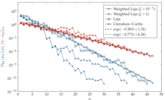
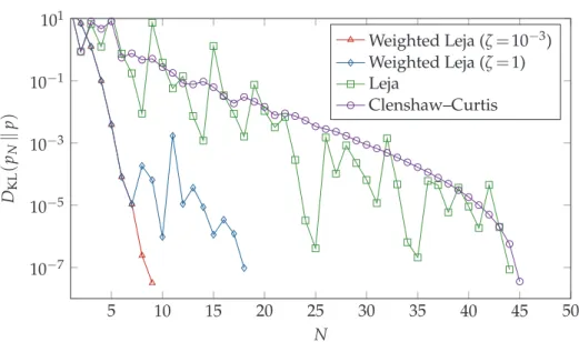
Three numerical test cases are employed to show the performance of our methodology. First, in Section 4.1 two explicit test cases are studied, which are cases where an expres-sion foruis known that can be evaluated accurately such that the exact posterior can be determined explicitly. We use these cases to verify the theoretical properties that have been derived in Section 3. For sake of comparison, these cases are studied using in-terpolation based on Clenshaw–Curtis nodes, Leja nodes, and the proposed adaptively weighted Leja nodes.

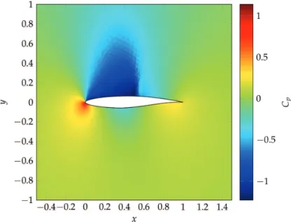
In Section 4.2, we study calibration of the one-dimensional Burgers’ equation. As an explicit solution is not used here, we can show the practical purposes of the interpol-ation procedure to problems that are defined implicitly. We determine the interpolant using Clenshaw–Curtis nodes and weighted Leja nodes. The last test case consists of the calibration of the closure parameters of the Spalart–Allmaras turbulence model. Here, a single evaluation of the likelihood is computationally expensive as it requires the numer-ical solution of the Navier–Stokes equations. In this case straightforward methods (such as MCMC) become intractable and therefore we will only study weighted Leja nodes.

Note that the quantity of interest in each case is the posterior and not the model. Therefore we mainly study the convergence in the posterior and to a lesser extent the convergence in the model.

4.1 Explicit test cases

We consider two analytic functions to demonstrate the applicability of the approach. Both functions are analytic in their domain of definition, but one of the functions cannot be represented globally by means of a power series expansion (which is often challenging in interpolation problems). The first function, a Gaussian function, has a large radius of convergence, such that a single power series expansion can be used to globally approx-imate the function accurately. The second function, a multi-variate extension of Runge’s function, yields a power series expansion with a small radius of convergence such that a single power series expansion cannot be used to globally approximate the function. Both functions are defined for any dimensiond.

4.1.1 Gaussian function

A well-known class of analytic functions is formed by Gaussian functions. We will use the following function to represent the model:

ud:[0,1]d→R, with ud(ϑ):=exp − d

∑

This function is a composition of the exponential function and a polynomial, which are both globally analytic. Hence also this function is globally analytic and can therefore

be approximated well using polynomials. Consequently, any nodal set can be used to interpolate this function—even an equidistant set—so we use this test case merely for a sanity check of the procedure and the theory.

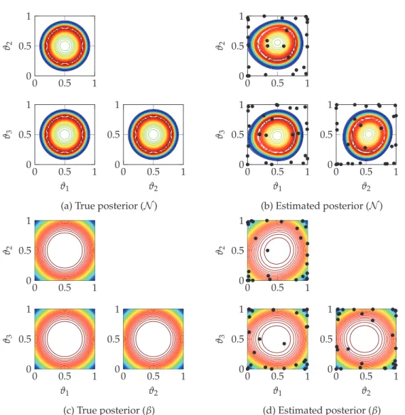
Two statistical models are employed to demonstrate the independence of our pro-cedure from the likelihood. The first is the statistical model discussed before, i.e.zk=

ud(ϑ)+εk, withε∼ N(0,Σ), Σ=σ2I, andσ=1/10. As discussed before, the likelihood

equals pN(z|ϑ)∝exp −1 2(z−ud(ϑ)) T_Σ−1_(z−u d(ϑ)) , (4.2)

wherezis the vector containing the data. A data vector ofn=20 elements is generated by sampling from a Gaussian distribution with mean ud(1/4) and standard deviation σ. The subscript N refers to multivariate normal. For the second model, we do not write an explicit relation between the data and the model, but only impose the following likelihood: pβ(z|ϑ)∝ ( (1−e)2_(1+e)2_{, if|e|<1} 0, otherwise, with e= z−ud(ϑ) z and z= 1 n n

∑

We call this likelihood the Beta likelihood (denoted withβ), which we use because it has different characteristics than the Gaussian likelihood. As the standard deviation is signi-ficantly larger in the second case, the posteriors differ considerably. Both likelihoods are continuously differentiable, so we expect similar accuracy when applying the proposed algorithm. In both cases the prior is assumed to be uniform on the domain[0,1]d_.

Because the model under consideration is analytic, the value ofζis not very important for the accuracy of the interpolation procedure (even ζ=0 works well in this case). We chooseζ=10−3_{, because then convergence of the posterior can be observed well, which}

is shown in Fig. 7 ford=3. It is clearly visible that for the multivariate normal case, the nodes are placed more in the center of the domain (see for comparison Fig. 2). This is also true for the second case, but less apparent due to the less intuitive structure of the posterior. The asymmetry between dimensions occurs due to the interpolation with Leja nodes, which are asymmetric by construction.

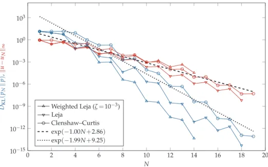
If we restrict ourselves to a one-dimensional case, the convergence of our algorithm can be assessed with high accuracy as it is possible to determine the Kullback–Leibler divergence with high accuracy using a quadrature rule. Moreover, a comparison with an interpolant based on Clenshaw–Curtis nodes can be performed. In higher dimensional cases such a comparison is not feasible, as determining the Kullback–Leibler divergence with high accuracy is intractable both with Monte Carlo (due to the relatively slow con-vergence) and with a quadrature rule (due to the deterioration of the high accuracy of the univariate quadrature rule). We want to emphasize here that assessing the convergence using the Kullback–Leibler divergence is essential, as the goal in this work is to construct an accurateposterior (and not necessary an accurateinterpolant, for which various more efficient multivariate interpolation techniques exist).