Transactions
[email protected] ISSN: 1696-2281
eISSN: 2013-8830 www.idescat.cat/sort/
A test for normality based on the empirical
distribution function
Hamzeh Torabi1, Narges H. Montazeri1and Aurea Gran´e2
Abstract
In this paper, a goodness-of-fit test for normality based on the comparison of the theoretical and empirical distributions is proposed. Critical values are obtained via Monte Carlo for several sample sizes and different significance levels. We study and compare the power of forty selected normality tests for a wide collection of alternative distributions. The new proposal is compared to some tradi-tional test statistics, such as Kolmogorov-Smirnov, Kuiper, Cram ´er-von Mises, Anderson-Darling, Pearson Chi-square, Shapiro-Wilk, Shapiro-Francia, Jarque-Bera, SJ, Robust Jarque-Bera, and also to entropy-based test statistics. From the simulation study results it is concluded that the best performance against asymmetric alternatives with support on the whole real line and alternative distributions with support on the positive real line is achieved by the new test. Other findings de-rived from the simulation study are that SJ and Robust Jarque-Bera tests are the most powerful ones for symmetric alternatives with support on the whole real line, whereas entropy-based tests are preferable for alternatives with support on the unit interval.
MSC: 62F03, 62F10.
Keywords: Empirical distribution function, entropy estimator, goodness-of-fit tests, Monte Carlo simulation, Robust Jarque-Bera test, Shapiro-Francia test, SJ test; test for normality.
1. Introduction
LetX1, . . . ,Xnbe anindependent an identically distributed (iid) random variables with continuous cumulative distribution function (cdf)F(.)and probability density function (pdf) f(.). All along the paper, we will denote the order statistic by (X(1), . . . ,X(n)).
Based on the observed samplex1, . . . ,xn, we are interested in the following goodness-of-fit test for a location-scale family:
1Statistics Department, Yazd University, 89175-741, Yazd, Iran, [email protected], [email protected] 2Statistics Department, Universidad Carlos III de Madrid, C/ Madrid 126, 28903 Getafe, Spain,
[email protected] Received: April 2015 Accepted: February 2016
H0: F∈F H1: F∈/F (1) where F = F0(.;θθθ) =F0 x−σµ
|θθθ= (µ, σ)∈Θ , Θ=R×(0,∞) and µ and σ are unspecified. The familyF is called location-scale family, whereF0(.)is the standard case forF0(.;θθθ)forθθθ= (0,1). Suppose that f0(x;θθθ) = σ1f0 x−σµ
is the corresponding pdf ofF0(x;θθθ).
The goodness-of-fit test problem for location-scale family described in (1) has been discussed by many authors. For instance, Zhao and Xu (2014) considered a random distance between the sample order statistic and the quasi sample order statistic derived from the null distribution as a measure of discrepancy. On the other hand, Alizadeh and Arghami (2012) used a test based on the minimum Kullback-Leibler distance. The Kullback-Leibler divergence measure is a special case of aφ-divergence measure (2) forφ(x) =xlog(x)−x+1 (see p. 5 of Pardo, 2006 for details). Alsoφ-divergence is a special case of theφ-disparity measure. Theφ-disparity measure between two pdf’s f0 and f is defined by Dφ(f0,f) = Z φ f0(x;θθθ) f(x) f(x)dx, (2)
whereφ:(0,∞)→[0,∞)is assumed to be continuous, decreasing on(0,1)and increas-ing on(1,∞), withφ(1) =0 (see p. 29 of Pardo, 2006 for details). Inφ-divergence,φis a convex function.
Inspired by this idea, in this paper we propose a goodness-of-fit statistic to test (1) by considering a new proximity measure between two continuous cdf’s. The organization of the paper is as follows. In Section 2 we define the new measure Hnand study its prop-erties as a goodness-of-fit statistic. In Section 3 we propose a normality test based on Hn and find its critical values for several sample sizes and different significance levels. In Section 4 we review forty normality tests, including the most traditional ones such as Kolmogorov-Smirnov, Cram´er-von Mises, Anderson-Darling, Wilk, Shapiro-Francia, Pearson Chi-square, among others, and in Section 5 we compare their perfor-mances to that of our proposal through a wide set of alternative distributions. We also provide an application example where the Kolmogorov-Smirnov test fails to detect the non normality of the sample.
2. A new discrepancy measure
In this section we define a discrepancy measure between two continuous cdf’s and study its properties as a goodness-of-fit statistic.
Definition 2.1 Let X and Y be two absolutely continuous random variables with cdf’s F0and F, respectively. We define
D(F0,F) = ∞ Z −∞ h 1+F0(x;θθθ) 1+F(x) dF(x) =EF h 1+F0(X;θθθ) 1+F(X) , (3)
where EF[.]is the expectation under F and h:(0,∞)→R+is assumed to be continuous, decreasing on(0,1)and increasing on(1,∞)with an absolute minimum at x=1such that h(1) =0.
Lemma 2.2D(F0,F)≥0and equality holds if and only if F0=F, almost everywhere. Proof. Using the non-negativity of functionh, we haveD(F0,F)≥0. It is clear thatF0= FimpliesD(F0,F) =0. Conversely, ifD(F0,F) =0, sincehhas an absolute minimum atx=1, thenF0=F.
Let us return to the goodness-of-fit test problem for a location-scale family described in (1). Firstly, we estimateµandσby their maximum likelihood estimators (MLEs), i.e.,
ˆ
µand ˆσ, respectively, and we takezi= (xi−µˆ)/σˆ,i=1, . . . ,n. Note that in this family, F0(xi; ˆµ,σˆ) =F0(zi). Secondly, consider the empirical distribution function (EDF) based on dataxi, that is Fn(t) = 1 n n X j=1 I[xj≤t],
where IA denotes the indicator of an event A. Then, our proposal is based on the ratio of the standard cdf underH0 and the EDF based on the xi’s. Using (3) with F =Fn, D(F0,Fn)can be written as Hn:=D(F0,Fn) = ∞ Z −∞ h 1+F0(x; ˆµ,σˆ) 1+Fn(x) dFn(x) = 1 n n X i=1 h 1+F0(x(i); ˆµ,σˆ) 1+Fn(x(i)) = 1 n n X i=1 h 1+F 0(z(i)) 1+i/n
UnderH0, we expect thatF0(t; ˆµ,σˆ)≈Fn(t), for everyt∈Rand 1+F0(t; ˆµ,σˆ)≈ 1+Fn(t). Note that, sinceh(1) =0, we expect thath (1+F0(t))/(1+Fn(t))
thus Hn will take values close to zero whenH0 is true. Therefore, it seems justifiable thatH0must be rejected for large values of Hn. Some standard choices forhare:h(x) = (x−1)2/(x+1)2,xlog(x)−x+1,(x−1)log(x),|x−1|or(x−1)2(for more examples, see p. 6 of Pardo, 2006 for details).
Proposition 2.3 The support ofHnis[0,max(h(1/2),h(2))].
Proof. SinceF0(.)andFnare cdf’s and take values in[0,1], we have that
1/2≤1+F0(y) 1+Fn(y) ≤ 2, y∈R. Thus 0≤h 1+F0(y) 1+Fn(y) ≤max(h(1/2),h(2))
Finally, since Hnis the mean ofh(.)over the transformed data, the result is obtained.
Proposition 2.4 The test statistic based onHnis invariant under location-scale trans-formations.
Proof. The location-scale family is invariant under the location-scale transformations of the formgc,r(X1, . . . ,Xn) = (rX1+c, . . . ,rXn+c),c∈R, r>0, which induces similar transformations onΘ:gc,r(θθθ) = (rµ+c,rσ)(See Shao, 2003). The estimatorT0(X1, . . . ,Xn) forµis location-scale invariant if
T0(rX1+c, . . . ,rXn+c) =rT0(X1, . . . ,Xn) +c, ∀r>0,c∈R, and the estimatorT1(X1, . . . ,Xn)forσis location-scale invariant if
T1(rX1+c, . . . ,rXn+c) =rT1(X1, . . . ,Xn), ∀r>0,c∈R.
We know that MLE ofµandσ are location-scale invariant for µandσ, respectively. Therefore underH0, the distribution ofZi= (Xi−µˆ)/σˆ does not depend onµandσ.
IfGnis the EDF based on datazi, then
Gn(zi) = 1 n n X j=1 I[zj≤zi]= 1 n n X j=1 I[xj≤xi]=Fn(xi),
therefore Hn= 1 n n X i=1 h 1+F 0(x(i); ˆµ,σˆ) 1+Fn(x(i)) = 1 n n X i=1 h 1+F 0(z(i)) 1+Gn(z(i)) .
Since the statistic Hn is a function ofzi, i=1, . . . ,n, is location-scale invariant. As a consequence, the null distribution of Hndoes not depend on the parametersµandσ.
Proposition 2.5 Let F1be an arbitrary continuous cdf in H1. Then under the assumption that the observed sample have cdf F1, the test based onHnis consistent.
Proof. Based on Glivenko-Cantelli theorem, fornlarge enough, we have thatFn(x)≃ F1(x), for allx∈R. Also ˆµand ˆσ are MLEs ofµ andσ, respectively, and hence are consistent. Therefore Hn= 1 n n X i=1 h 1+F 0(x(i); ˆµ,σˆ) 1+Fn(x(i)) =1 n n X i=1 h 1+F0(xi; ˆµ,σˆ) 1+Fn(xi) ≃1n n X i=1 h 1+F0(xi; ˆµ,σˆ) 1+F1(xi) ≃1n n X i=1 h 1+F0(xi, µ, σ) 1+F1(xi) →EF1 h 1+F0(X, µ, σ) 1+F1(X) =:D(F0,F1), asn→∞,
whereEF1[.]is the expectation underF1, andµandσ2are, respectively, the expectation and variance ofF1. Note that the convergence holds by the law of large numbers and D(F0,F1)is a divergence betweenF0andF1. So the test based on Hnis consistent.
3. A normality test based on
H
nMany statistical procedures are based on the assumption that the observed data are nor-mally distributed. Consequently, a variety of tests have been developed to check the validity of this assumption. In this section, we propose a new normality test based on Hn.
Consider again the goodness-of-fit testing problem described in (1), where now f0(x;µ, σ) =1/
√
2πσ2e−(x−µ)2/2σ2
,x∈R, in whichµ∈Randσ>0 are both unknown, andF0(.;µ, σ)is the corresponding cdf, whereF0(.)is the standard case forF0(.; 0,1).
First we estimateµandσby their maximum likelihood estimators (MLEs), i.e., ˆµ= ¯
x=1/nPn
i=1xiand ˆσ2=s2=1/(n−1)
Pn
i=1(xi−x)¯ 2, respectively. Letzi= (xi−x)¯ /s, i=1, . . . ,n. Then, the test statistic for normality is:
Hn= 1 n n X i=1 h 1+ F0(x(i),x¯,s) 1+Fn(x(i)) =1 n n X i=1 h 1+ F0(z(i)) 1+i/n , (4) where h(x) = x−1 x+1 2 . (5)
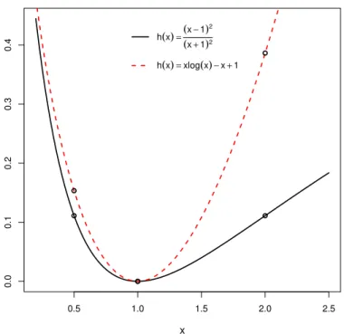
Note thath:(0,∞)→R+ is decreasing on(0,1)and increasing on(1,∞) with an ab-solute minimum atx=1 such thath(1) =0 (see Figure 1). We selected this function h, because based on simulation study, it is more powerful than other functionsh. For example, we consideredh2(x):=xlog(x)−x+1 for comparison withh1(x):= xx−+11
2 (see Tables 6 and 7).
Corollary 3.1 The support ofHnis[0,0.11].
Proof. From Proposition 2.3 and Figure 1, max(h(1/2),h(2)) =0.11.
Table 1 contains the upper critical values of Hn, which have obtained by Monte Carlo from 100000 simulated samples for different sample sizes n and significance levels α=0.01,0.05,0.1. 0.5 1.0 1.5 2.0 2.5 0.0 0.1 0.2 0.3 0.4 x h(x)=(x−1) 2 (x+1)2 h(x)=xlog(x)−x+1
Table 1: Critical values ofHnforα=0.01,0.05,0.1. n 5 6 7 8 9 10 15 20 25 30 40 50 α 0.01 .0039 .0035 .0030 .0026 .0023 .0021 .0014 .0011 .0008 .0007 .0005 .0004 0.05 .0030 .0026 .0022 .0019 .0017 .0016 .0010 .0007 .0006 .0005 .0004 .0003 0.10 .0026 .0022 .0019 .0016 .0015 .0013 .0009 .0006 .0005 .0004 .0003 .0002
Remember that, Hnis expected to take values close to zero whenH0is true. Hence, H0 will be rejected for large values of Hn. Also Hn is invariant under location-scale transformations and consistent under the assumptionH1, respectively, from Propositions 2.4 and 2.5.
4. Normality tests under evaluation
Comparison of the normality tests has received attention in the literature The goodness-of-fit tests have been discussed by many authors including Shapiro et al. (1968), Poitras (2006), Yazici and Yolacan (2007), Krauczi (2009), Romao et al. (2010), Yap and Sim (2010) and Alizadeh and Arghami (2011).
In this section we consider a large number (forty) of recent and classical statistics that have been used to test normality and in Section 5 we compare their performances with that of Hn. In the following we prefer to keep the original notation for each statistic. Con-cerning the notation, letx1,x2, . . . ,xnbe a random sample of sizenandx(1),x(2), . . . ,x(n)
the corresponding order statistic. Also consider the sample mean, variance, skewness and kurtosis, defined by
¯ x= 1 n n X i=1 xi, s2= 1 n n X i=1 (xi−x)¯ 2, p b1= m3 (m2)3/2 , b2= m4 (m2)2 ,
respectively, where the j-th central moment mj is given by mj = 1nPni=1(xi−x)¯ j and finally considerz(i)= (x(i)−x)¯ /s, fori=1, . . . ,n.
1. Vasicek’s entropy estimator (Vasicek, 1976):
KLmn= exp{HVmn} s where HVmn= 1 n n X i=1 lnn n 2m X(i+m)−X(i−m) o , (6)
m<n/2 is a positive integer andX(i)=X(1)ifi<1 andX(i)=X(n)ifi>n.H0is rejected for small values of KL. Vasicek (1976) showed that the maximum power for KL was typically attained by choosingm=2 forn=10,m=3 forn=20 and m=4 forn=50. The lower-tail 5%-significance values of KL forn=10,20 and 50 are 2.15, 2.77 and 3.34, respectively.
2. Ebrahimi’s entropy estimator (Ebrahimi, Pflughoeft and Soofi, 1994):
TEmn= exp{HEmn} s , where HEmn= 1 n n X i=1 ln n cim X(i+m)−X(i−m) , (7)
andci= (1+i−m1)I[1,m](i) +2I[m+1,n−m](i) + (1+nm−i)I[n−m+1,n](i). Ebrahimi et al.
(1994) proved the linear relationship between their estimator and (6). Thus for fixed values ofnandm, the tests based on (6) and (7) have the same power. 3. Nonparametric distribution function of Vasicek’s estimator:
TVmn=log q
2πσˆ2
v+0.5−HVmn, where HVmnwas defined in (6), ˆσ2v=Vargv(X), and
gv(x) = 0 x< ξ1 or x> ξn+1, 2m n(x(i+m)−x(i−m)) ξi<x≤ξi+1 i=1, . . . ,n, whereξi= x(i−m)+···+x(i+m−1)
/2m.H0is rejected for large values of TVmn. (See Park, 2003).
4. Nonparametric distribution function of Ebrahimi estimator: TEmn=log
q 2πσˆ2
e+0.5−HEmn, where HEmnwas defined in (7), ˆσ2e =Varge(X)and
ge(x) = (
0 x< η1 or x> ηn+1 1
with ηi= ξm+1−m+1k−1 Pm k=i(x(m+k)−x(1)) 1≤i≤m, 1 2m x(i−m)+···+x(i+m−1) m+1≤i≤n−m+1, ξn−m+1+n+m1−k+1 Pi k=n−m+2(x(n)−x(k−m−1)) n−m+2≤i≤n+1, andξi= x(i−m)+···+x(i+m−1)
/2m.H0is rejected for large values of TEmn. (See Park, 2003).
5. Nonparametric distribution function of Alizadeh and Arghami estimator (Alizadeh Noughabi and Arghami, 2010, 2013): TAmn=log q 2πσˆ2 a+0.5−HAmn, where HAmn= 1 n n X i=1 ln n aim X(i+m)−X(i−m) ,
withai=I[1,m](i) +2I[m+1,n−m](i) +I[n−m+1,n](i), ˆσa2=Varga(X)and
ga(x) = ( 0 x< η1 or x> ηn+1, 1 n(ηi+1−ηi) ηi<x≤ηi+1 i=1, . . . ,n, with ηi= ξm+1−m1Pmk=i(x(m+k)−x(1)) 1≤i≤m, 1 2m x(i−m)+···+x(i+m−1) m+1≤i≤n−m+1, ξn−m+1+m1 Pi k=n−m+2(x(n)−x(k−m−1)) n−m+2≤i≤n+1, andξi= x(i−m)+···+x(i+m−1)
/2m. Alsom= [√n+1].H0is rejected for large values of TAmn. The upper-tail 5%-significance values of TA forn=10,20 and 50 are 0.4422, 0.2805 and 0.1805, respectively.
6. Dimitriev and Tarasenko’s entropy estimator (Dimitriev and Tarasenko, 1973):
TDmn=
exp{HDmn} s
where HDmn=− ∞ Z −∞ ln(f(x))ˆ f(x)ˆ dx,
where ˆf(x)is the kernel density estimation of f(x)given by
ˆ f(Xi) = 1 nh n X j=1 k Xi−Xj h , (8)
wherekis a kernel function satisfyingR−∞∞k(x)dx=1 andhis a bandwidth. The kernel functionk being the standard normal density function and the bandwidth h=1.06 ˆσn−1/5.H
0is rejected for small values of TDmn. 7. Corea’s entropy estimator (Corea, 1995):
TCmn= exp{HCmn} s , where HCmn=− 1 n n X i=1 ln ( Pi+m j=i−m X(j)−X˜(i) (j−i) nPi+m j=i−m X(j)−X˜(i) 2 )
and ˜X(i)=Pij+=mi−mX(j)/(2m+1).H0is rejected for small values of TCmn. 8. Van Es’s entropy estimator (Van Es, 1992):
TEsmn= exp{HEsmn} s , where HEsmn= 1 n−m n−m X i=1 ln n+1 m (X(i+m)−X(i)) + n X k=m 1 k+ln(m)−ln(n+1).
H0is rejected for small values of TEsmn.
9. Zamanzade and Arghami’s entropy estimator (Zamanzade and Arghami, 2012):
TZ1mn=
exp{HZ1mn}
where HZ1mn=1nPni=1ln(bi), with bi= X(i+m)−X(i−m) Pk2(i)−1 j=k1(i)( ˆ f(X(j+1)) +f(Xˆ (j)))(X(j+1)−X(j))/2 (9)
where ˆf is defined as in (8) with the kernel functionk being the standard normal density function and the bandwidthh=1.06 ˆσn−1/5.H
0is rejected for small values of TZ1. Forn=10,20 and 50, the lower-tail 5%-significance critical values are 3.403, 3.648 and 3.867.
10. Zamanzade and Arghami’s entropy estimator (Zamanzade and Arghami, 2012):
TZ2mn=
exp{HZ2mn}
s ,
where HZ2mn=Pni=1wiln(bi), being coefficientsbi’s were defined in (9) and
wi= (m+i−1)/Pn i=1wi 1≤i≤m, 2m/Pn i=1wi m+1≤i≤n−m, (n−i+m)/Pn i=1wi n−m+1≤i≤n, i=1, . . . ,n,
are weights proportional to the number of points used in computation ofbi’s.H0 is rejected for small values of TZ2. For n =10,20 and 50, the lower-tail 5%-significance critical values are 3.321, 3.520 and 3.721.
11. Zhang and Wu’s statistics (Zhang and Wu, 2005):
ZK= max 1≤i≤n (i−0.5)ln i−0.5 nF0(Z(i)) + (n−i+0.5)ln n−i+0.5 n(1−F0(Z(i))) , ZC= n X i=1 log (1/F0(Z(i))−1) (n−0.5)/(i−0.75)−1 2 , and ZA=− n X i=1 logF0(Z(i)) n−i+0.5 + log(1−F0(Z(i)) i−0.5 ,
12. Classical test statistics for normality based skewness and kurtosis from D’Agostino and Pearson (D’Agostino and Pearson, 1973):
p b1= m3 (m2)3/2 , b2= m4 (m2)2 ,
The null hypothesisH0is rejected for both small and large values of the two test statistics.
13. Transformed skewness and kurtosis statistic from D’Agostino et al. (1990):
K2=hZ(pb1) i2 + [Z(b2)]2, where Z(pb1) = log(Y/c+p (Y/c)2+1) p log(w) , Z(b2) = " 1− 2 9A − 3 s 1−2/A 1+yp2/(A−4) # r 9A 2 , where c1=6+8/c2(2/c2+ q 1+4/c22), c2= (6(n2−5n+2)/(n+7)(n+9)) p 6(n+3)(n+5)/n(n−2)(n−3), c3= (b2−3(n−1)/(n+1))/ q 24n(n−2)(n−3)/(n+1)2(n+3)(n+5). and Y =pb1 s (n+1)(n+3) 6(n−2) , w 2=p 2β2−1−1, β2= 3(n2+27n−70)(n+1)(n+3) (n−2)(n+5)(n+7)(n+9) ; c= s 2 (w2−1).
Transformed skewness Z(√b1) and transformed kurtosis Z(b2) is obtained by D’Agostino (1970) and Anscombe and Glynn (1983), respectively. The null hy-pothesisH0is rejected for large values of K2.
14. Transformed skewness and kurtosis statistic by Doornik and Hansen (1994): DH=hZ(pb1) i2 +z22, where z2= " ξ 2a 1/3 −1+ 1 9a # √ 9a, and ξ= (b2−1−b1)2k, k=(n+5)(n+7)(n 3+37n2+11n−313) 12(n−3)(n+1)(n2+15n−4) , a=(n+5)(n+7) (n−2)(n 2+27n−70) +b 1(n−7)(n2+2n−5) 6(n−3)(n+1)(n2+15n−4) ,
Transformed kurtosis z2 is obtained by Shenton and Bowman (1977). The null hypothesisH0is rejected for large values of DH.
15. Bonett and Seier’s statistic (Bonett and Seier, 2002):
Zw= √ n+2(wˆ−3) 3.54 , where ˆw=13.29 ln√m2−log n−1 Pn i=1|xi−x¯|
.H0is rejected for both small and large values of Zw.
16. D’Agostino’s statistic (D’Agostino, 1971):
D= Pn i=1(i−(n+1)/2)X(i) n2 q Pn i=1 x(i)−X¯2 ,
H0is rejected for both small and large values of D. 17. Chen and Shapiro’s statistic (Chen and Shapiro, 1995):
QH= 1 (n−1)s n−1 X i=1 X(i+1)−X(i) M(i+1)−M(i) ,
whereMi=Φ−1((i−0.375)/(n+0.25)), whereΦis the cdf of a standard normal random variable.H0is rejected for small values of QH.
18. Filliben’s statistic (Filliben, 1975):
r= Pn i=1x(i)M(i) q Pn i=1M(2i) p (n−1)s2,
whereM(i)=Φ−1(m(i))andm(1)=1−0.51/n,m(n)=0.51/nandm(i)= (i−0.3175)/(n+
0.365)fori=2, . . . ,n−1.H0is rejected for small values of r. 19. del Barrio et al.’s statistic (del Barrio et al., 1999):
Rn=1− Pn k=1X(k) Rk/n (k−1)/nF− 1 0 (t)dt 2 m2 ,
wherem2is the sample standardized second moment.H0is rejected for large val-ues of Rn.
20. Epps and Pulley statistic (Epps and Pulley, 1983):
TEP= 1 √ 3+ 1 n2 n X k=1 n X j=1 exp −(Xj−Xk)2 2m2 − √ 2 n n X j=1 exp −(Xj−X¯)2 4m2 ,
wherem2is the sample standardized second moment.H0is rejected for large val-ues of TEP.
21. Martinez and Iglewicz’s statistic (Martinez and Iglewicz, 1981):
In= Pn i=1(Xi−M)2 (n−1)S2 b ,
whereMis is the sample median and
S2b= nP |Z˜i|<1(Xi−M) 2(1−Z˜2 i)4 P |Z˜i|<1(1−Z˜i2)(1−5 ˜Zi2) 2,
with ˜Zi= (Xi−M)/(9A)for|Z˜i|<1 and ˜Zi=0 otherwise, andAis the median of
22. deWet and Venter statistic (de Wet and Venter, 1972): En= n X i=1 X(i)−X¯−sΦ−1 i n+1 2 s2.
H0is rejected for large values of En. 23. Optimal test (Cs ¨orgo and R´ev´esz, 1971):
Mn= n X i=1 X(i)−X¯−sΦ−1 i n+1 2 φ Φ−1 i n+1 Φ −1 i n+1 λ−1 .
H0is rejected for large values of Mn. 24. Pettitt statistic (Pettitt, 1977):
Qn= n X i=1 Φ X (i)−X¯ s −n+i 1 2 φ Φ−1 i n+1 −2 .
H0is rejected for large values of Qn. 25. Three test statistics from LaRiccia (1986):
T1n=C12n/(s2B1n), T2n=C22n/(s2B2n), T3n=T1n+T2n, where C1n= 1 √ n n X i=1 W1 i n+1 −A1n X(i), C2n= 1 √ n n X i=1 W2 i n+1 −A2nΦ−1 i n+1 X(i),
AlsoW1(u) = [Φ−1(u)]2−1 andW2(u) = [Φ−1(u)]3−3Φ−1(u). The constantsA1n, A2n,B1nandB2nare given in Table 1 from LaRiccia (1986). For all three statistics H0is rejected for large value.
26. Kolmogorov-Smirnov’s (Lilliefors) statistic (Kolmogorov, 1933):
KS=max max 1≤j≤n j n−F0(Z(j)) ,max 1≤j≤n F0(Z(j))− j−1 n .
Lilliefors (1967) computed estimated critical points for the Kolmogorov-Smirnov’s test statistic for testing normality when mean and variance estimated.
27. Kuiper’s statistic (Kuiper, 1962):
V= max 1≤j≤n j n−F0(Z(j)) + max 1≤j≤n F0(Z(j))− j−1 n .
Louter and Kort (1970) computed estimated critical points for the Kuiper test statistic for testing normality when mean and variance estimated.
28. Cram´er-von Mises’ statistic (Cram´er, 1928 and von Mises, 1931):
W2= 1 12n+ n X j=1 F0(Z(j))− 2j−1 2n 2 .
29. Watson’s statistic (Watson, 1961):
U2=W2−n 1 n n X j=1 F0(Z(j))− 1 2 2 .
30. Anderson-Darling’s statistic (Anderson, 1954):
A2=−n−1 n
n X
i=1
(2i−1) log(F0(Z(i))) +log 1−F0(Z(n−i+1))
.
These classical tests are based on the empirical distribution function andH0 is rejected for large values of KS, V, W2, U2and A2.
31. Pearson’s chi-square statistic (D’Agostino and Stephens, 1986):
P=X
i
(Ci−Ei)2/Ei,
whereCi is the number of counted andEiis the number of expected observations (underH0) in classi. The classes are build is such a way that they are equiprobable under the null hypothesis of normality. The number of classes used for the test is
32. Shapiro-Wilk’s statistic (Shapiro and Wilk, 1965): SW= P[n/2] i=1 a(n−i+1) X(n−i+1)−X(i) 2 Pn i=1 X(i)−X¯ 2 ,
where coefficientsai’s are given by
(a1, . . . ,an) =
mTV−1
(mTV−1V−1m)1/2, (10) andmT = (m1, . . . ,mn)andV are, respectively, the vector of expected values and the covariance matrix of the order statistic ofniid random variables sampled from the standard normal distribution.H0is rejected for small values of SW.
33. Shapiro-Francia’s statistic (Shapiro and Francia, 1972) is a modification of SW. It is defined as SF= Pn i=1biX(i)2 Pn i=1(X(i)−X¯)2 , where (b1, . . . ,bn) = mT (mTm)1/2
andmis defined as in (10).H0is rejected for small values of SF.
34. SJ statistic discussed in Gel, Miao and Gastwirth (2007). It is based on the ratio of the classical standard deviation ˆσand the robust standard deviationJn(average absolute deviation from the median (MAAD)) of the sample data
SJ= s Jn , (11) where Jn= pπ 2 1 n Pn
i=1|Xi−M|andM is the sample median.H0 is rejected for large values of SJ.
35. Jarque-Bera’s statistic (Jarque and Bera, 1980, 1987): JB=n
6b1+ n
24(b2−3)
where√b1andb2are the sample skewness and sample kurtosis, respectively.H0 is rejected for large values of JB.
36. Robust Jarque-Bera’s statistic (Gel and Gastwirth, 2008):
RJB= n C1 m3 J3 n 2 + n C2 m4 J4 n − 3 2 ,
whereJnis defined as in (11),C1andC2are positive constants. For a 5%-significance level,C1=6 andC2=64 according to Monte Carlo simulations.H0is rejected for large values of RJB.
5. Simulation study
In this section we study the power of the normality test based on Hnand compare it with a large number of recent and classical normality tests. To facilitate comparisons of the power of the present test with the powers of the mentioned tests, we select two sets of alternative distributions:
Set 1.Alternatives listed in in Esteban et al. (2001).
Set 2.Alternatives listed in Gan and Koehler (1990) and Krauczi (2009).
Set 1 of alternative distributions
Following Esteban et al. (2001) we consider the following alternative distributions, that can be classified in four groups:
Group I: Symmetric distributions with support on(−∞,∞):
• Standard Normal (N);
• Student’st(t) with 1 and 3 degrees of freedoms;
• Double Exponential (DE) with parametersµ=0 (location) andσ=1 (scale);
• Logistic (L) with parametersµ=0 (location) andσ=1 (scale); Group II: Asymmetric distributions with support on(−∞,∞):
• Gumbel (Gu) with parametersα=0 (location) andβ=1 (scale);
• Skew Normal (SN) with with parametersµ=0 (location),σ=1 (scale) and α=2 (shape);
Group III: Distributions with support on(0,∞):
• Exponential (Exp) with mean 1;
• Gamma (G) with parametersβ=1 (scale) andα=.5,2 (shape);
• Lognormal (LN) with parametersµ=0 andσ=.5,1,2;
• Weibull (W) with parametersβ=1 (scale) andα=.5,2 (shape); Group IV: Distributions with support on(0,1):
• Uniform (Unif);
• Beta (B) with parameters (2,2), (.5,.5), (3,1.5) and (2,1). Set 2 of alternative distributions
Gan and Koehler (1990) and Krauczi (2009) considered a battery of “difficult alterna-tives” for comparing normality tests. We also consider them in order to evaluate the sensitivity of the proposed test. LetU andZ denote a [0,1]-Uniform and a Standard Normal random variable, respectively.
• Contaminated Normal distribution (CN) with parameters(λ, µ1, µ2, σ) given by the cdfF(x) = (1−λ)F0(x, µ1,1) +λF0(x, µ2, σ);
• Half Normal (HN) distribution, that is, the distribution of|Z|.
• Bounded Johnson’s distribution (SB) with parameters(γ, δ)of the random variable e(Z−γ)/δ/(1+e(Z−γ)/δ);
• Unbounded Johnson’s distribution (UB) with parameters(γ, δ)of the random vari-able sinh((Z−γ)/δ);
• Triangle type I (Tri) with density function f(x) =1− |t|,−1<t<1;
• Truncated Standard Normal distribution ataandb(TN);
• Tukey’s distribution (Tu) with parameterλof the random variableUλ−(1−U)λ. • Cauchy distribution with parametersµ=0 (location),σ=1 (scale).
• Chi-squared distributionχ2withkdegrees of freedom.
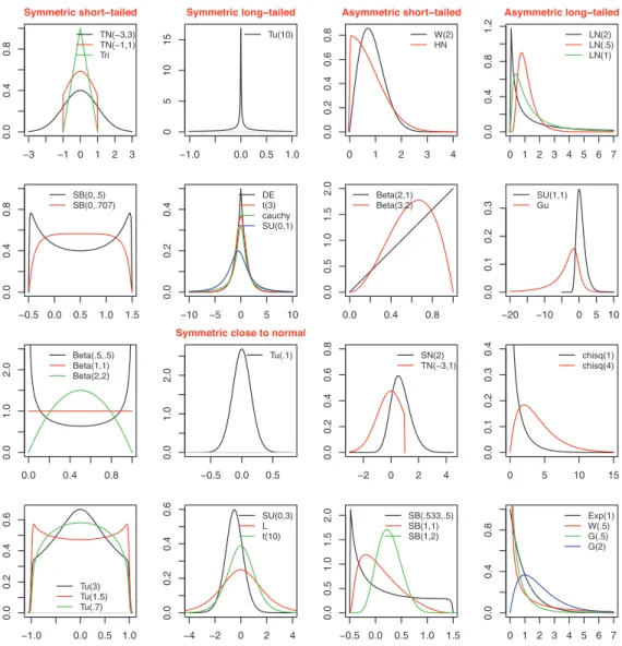
Tables 2-3 contain the skewness(√β1)and kurtosis(β2)of the previous sets of alter-native distributions. Alteralter-natives inSet 2are roughly ordered and grouped in five groups according to their skewness and kurtosis values in Table 3. These groups correspond to: symmetric short tailed, symmetric closed to normal, asymmetric short tailed, asym-metric long tailed. Figure 2 illustrates some of the possible shapes of the pdf’s of the alternatives inSet 1andSet 2.
−3 −1 0 1 2 3 0.0 0.4 0.8 Symmetric short−tailed TN(−3,3) TN(−1,1) Tri −0.5 0.0 0.5 1.0 1.5 0.0 0.4 0.8 SB(0,.5) SB(0,.707) 0.0 0.4 0.8 0.0 1.0 2.0 Beta(.5,.5) Beta(1,1) Beta(2,2) −1.0 0.0 0.5 1.0 0.0 0.2 0.4 0.6 Tu(3) Tu(1.5) Tu(.7) −1.0 0.0 0.5 1.0 0 5 10 15 Symmetric long−tailed Tu(10) −10 −5 0 5 10 0.0 0.2 0.4 DE t(3) cauchy SU(0,1) −0.5 0.0 0.5 0.0 1.0 2.0
Symmetric close to normal Tu(.1) −4 −2 0 2 4 0.0 0.2 0.4 0.6 SU(0,3) L t(10) 0 1 2 3 4 0.0 0.2 0.4 0.6 0.8 Asymmetric short−tailed W(2) HN 0.0 0.4 0.8 0.0 0.5 1.0 1.5 2.0 Beta(2,1) Beta(3,2) −2 0 2 4 0.0 0.2 0.4 0.6 0.8 SN(2) TN(−3,1) −0.5 0.0 0.5 1.0 1.5 0.0 0.5 1.0 1.5 2.0 SB(.533,.5) SB(1,1) SB(1,2) 0 1 2 3 4 5 6 7 0.0 0.4 0.8 1.2 Asymmetric long−tailed LN(2) LN(.5) LN(1) −20 −10 0 5 10 0.0 0.1 0.2 0.3 SU(1,1) Gu 0 5 10 15 0.0 0.1 0.2 0.3 0.4 chisq(1) chisq(4) 0 1 2 3 4 5 6 7 0.0 0.4 0.8 Exp(1) W(.5) G(.5) G(2)
Figure 2: Plots of alternative distributions inSet 1andSet 2.
Tables 4-5 contain the estimated value of Hn(forh(x) = (x−1)2/(x+1)2andh(x) = xlog(x)−x+1, respectively), for each alternative distribution, computed as the average value from 10000 simulated samples of sizesn=10,20,50,100,1000. In the last row of these tables(n=∞)), we show the value ofD(F0,F1)computed with the the command
integratein R Software, with(µ)and(σ2)being the expectation and variance ofF
1,
respectively.These tables show consistency of the test statisticHn.
Tables 6-7 report the power of the 5% significance level of forty normality tests based on the statistics considered in Section 4 for theSet 1of alternatives.
Tables 8-9 contain the power of the 5% significance level test of normality based on the most powerful statistics and the alternatives listed inSet 2.
T a b le 2 : S ke w n es s a n d ku rt o si s o f a lt er n a ti ve d is tr ib u ti o n s in S et 1 . G ro u p I G ro u p II G ro u p II I G ro u p IV t( 1 ) t( 3 ) L D E G u S N (2 ) E x p G (2 ) G (. 5 ) L N (1 ) L N (2 ) L N (. 5 ) W (. 5 ) W (2 ) U n if B (2 ,2 ) B (. 5 ,. 5 ) B (3 ,. 5 ) B (2 ,1 ) √ β 1 0 0 0 0 1 .3 0 .4 5 2 1 .4 1 2 .8 3 6 .1 8 4 1 4 .3 6 1 .7 5 6 .6 2 .6 3 0 0 0 − 1 .5 7 5 − .5 7 β2 — — 4 .2 6 5 .4 .3 1 9 6 1 5 1 1 3 .9 4 9 2 2 0 5 6 0 8 .9 0 8 7 .7 2 3 .2 5 1 .8 2 .1 4 1 .5 5 .2 2 2 .4 T a b le 3 : S ke w n es s a n d ku rt o si s o f a lt er n a ti ve d is tr ib u ti o n s in S et 2 . S y m m et ri c A sy m m et ri c S h o rt ta il ed C lo se to N o rm al L o n g ta il ed S h o rt ta il ed L o n g ta il ed T u T u T u S B T ri T N T N T u S U t T u S U ca u sh y T N S B S B S B H N S U χ 2 χ 2 (. 7 ) (1 .5 ) (3 ) (0 ,. 5 ) ( − 1 ,1 ) ( − 3 ,3 ) (. 1 ) (0 ,3 ) (1 0 ) (1 0 ) (0 ,1 ) ( − 3 ,1 ) (1 ,1 ) (1 ,2 ) (. 5 3 3 ,. 5 ) (1 ,1 ) ( 1 ) ( 4 ) √ β 1 0 0 0 0 0 0 0 0 0 0 0 0 0 − .5 5 .7 3 .2 8 .6 5 .9 7 − 5 .3 7 2 .8 3 1 .4 1 β2 1 .9 2 1 .7 5 2 .0 6 1 .6 3 2 .4 1 .9 4 2 .8 4 3 .2 1 3 .5 3 4 5 .3 8 3 6 .2 ∞ 2 .7 8 2 .9 1 2 .7 7 2 .1 3 3 .7 8 9 3 .4 1 5 6
T a b le 4 : E st im a te d va lu e o f Hn w it h h1 ( x ) = ( x − 1 ) 2/ ( x + 1 ) 2u n d er H1 , b a se d o n 1 0 0 0 0 si m u la ti o n s fo r se ve ra l va lu es o f n . G ro u p I G ro u p II G ro u p II I G ro u p IV t( 1 ) t( 3 ) L D E G u S N (2 ) E x p G (2 ) G (. 5 ) L N (1 ) L N (2 ) L N (. 5 ) W (. 5 ) W (2 ) U n if B (2 ,2 ) B (. 5 ,. 5 ) B (3 ,. 5 ) B (2 ,1 ) n 10 — .0 0 1 1 .0 0 0 8 6 .0 0 1 0 .0 0 1 1 .0 0 0 9 2 .0 0 1 7 .0 0 1 3 .0 0 2 5 .0 0 2 2 6 .0 0 4 0 .0 0 1 3 .0 0 3 5 .0 0 0 9 7 .0 0 0 9 .0 0 0 8 2 .0 0 1 2 .0 0 1 3 .0 0 0 8 2 0 — .0 0 0 7 .0 0 0 4 3 .0 0 0 6 .0 0 0 7 .0 0 0 4 7 .0 0 1 4 .0 0 0 9 .0 0 2 3 .0 0 2 1 3 .0 0 4 5 .0 0 0 9 .0 0 3 6 .0 0 0 5 4 .0 0 0 5 .0 0 0 4 1 .0 0 0 8 .0 0 1 1 .0 0 0 5 5 0 — .0 0 0 5 .0 0 0 1 8 .0 0 0 4 .0 0 0 4 .0 0 0 2 2 .0 0 1 2 .0 0 0 6 .0 0 2 2 .0 0 2 1 1 .0 0 5 2 .0 0 0 7 .0 0 3 7 .0 0 0 2 8 .0 0 0 3 .0 0 0 1 9 .0 0 0 6 .0 0 1 1 .0 0 0 3 1 0 0 — .0 0 0 4 .0 0 0 1 1 .0 0 0 3 .0 0 0 3 .0 0 0 1 3 .0 0 1 1 .0 0 0 6 .0 0 2 2 .0 0 2 1 5 .0 0 5 6 .0 0 0 6 .0 0 3 9 .0 0 0 1 9 .0 0 0 3 .0 0 0 1 2 .0 0 0 6 .0 0 1 1 .0 0 0 3 1 0 0 0 — .0 0 0 4 .0 0 0 0 4 .0 0 0 2 .0 0 0 2 .0 0 0 0 6 .0 0 1 0 .0 0 0 5 .0 0 2 1 .0 0 2 2 6 .0 0 6 6 .0 0 0 5 .0 0 4 0 .0 0 0 1 2 .0 0 0 2 .0 0 0 0 6 .0 0 0 5 .0 0 1 1 .0 0 0 2 ∞ — .0 0 0 4 .0 0 0 0 3 .0 0 0 2 .0 0 0 2 .0 0 0 0 5 .0 0 1 0 .0 0 0 5 .0 0 2 1 .0 0 2 2 8 .0 0 7 4 .0 0 0 5 .0 0 4 0 .0 0 0 1 1 .0 0 0 2 .0 0 0 0 6 .0 0 0 5 .0 0 1 1 .0 0 0 2 T a b le 5 : E st im a te d va lu e o f Hn w it h h2 ( x ) = x lo g ( x ) − x + 1 u n d er H1 , b a se d o n 1 0 0 0 0 si m u la ti o n s fo r se ve ra l va lu es o f n . G ro u p I G ro u p II G ro u p II I G ro u p IV t( 1 ) t( 3 ) L D E G u S N (2 ) E x p G (2 ) G (. 5 ) L N (1 ) L N (2 ) L N (. 5 ) W (. 5 ) W (2 ) U n if B (2 ,2 ) B (. 5 ,. 5 ) B (3 ,. 5 ) B (2 ,1 ) n 10 — .0 0 2 1 .0 0 1 6 7 .0 0 1 9 .0 0 2 2 .0 0 1 8 .0 0 3 4 .0 0 2 7 .0 0 4 8 .0 0 4 4 .0 0 7 7 .0 0 2 6 .0 0 6 5 .0 0 2 0 .0 0 1 9 .0 0 1 7 .0 0 2 5 .0 0 2 7 .0 0 1 7 2 0 — .0 0 1 4 .0 0 0 8 6 .0 0 1 2 .0 0 1 3 .0 0 0 9 .0 0 2 8 .0 0 1 7 .0 0 4 5 .0 0 4 2 .0 0 8 8 .0 0 1 8 .0 0 7 0 .0 0 1 0 .0 0 1 1 .0 0 0 9 .0 0 1 7 .0 0 2 4 .0 0 1 0 5 0 -.0 0 1 0 .0 0 0 3 7 .0 0 0 7 .0 0 0 8 .0 0 0 4 .0 0 2 3 .0 0 1 3 .0 0 4 4 .0 0 4 2 .0 1 0 6 .0 0 1 3 .0 0 7 5 .0 0 0 5 .0 0 0 6 .0 0 0 4 .0 0 1 3 .0 0 2 3 .0 0 0 6 1 0 0 -.0 0 0 9 .0 0 0 2 1 .0 0 0 6 .0 0 0 6 .0 0 0 3 .0 0 2 2 .0 0 1 .0 0 4 3 .0 0 4 3 .0 1 1 3 .0 0 1 2 .0 0 7 9 .0 0 0 4 .0 0 0 5 .0 0 0 3 .0 0 1 2 .0 0 2 3 .0 0 0 5 1 0 0 0 — .0 0 0 9 .0 0 0 0 7 .0 0 0 4 .0 0 0 5 .0 0 0 1 .0 0 2 1 .0 0 0 9 .0 0 4 3 .0 0 4 6 .0 1 3 9 .0 0 1 0 .0 0 8 4 .0 0 0 2 .0 0 0 4 .0 0 0 1 .0 0 1 1 .0 0 2 3 .0 0 0 4 ∞ — .0 0 0 9 .0 0 0 0 6 .0 0 0 4 .0 0 0 5 .0 0 0 1 .0 0 2 1 .0 0 0 9 .0 0 4 3 .0 0 4 7 .0 1 6 3 .0 0 1 0 .0 0 8 4 .0 0 0 2 .0 0 0 4 .0 0 0 1 .0 0 1 0 .0 0 2 3 .0 0 0 4
T a b le 6 : P o w er co m p a ri so n s fo r th e n o rm a li ty te st fo r S et 1 o f a lt er n a ti ve d is tr ib u ti o n s, α = 0 . 0 5 , n = 1 0 . G ro u p I II II I IV al te rn . N t( 1 ) t( 3 ) L D E G u S N E x p G (2 ) G (. 5 ) L N (1 ) L N (2 ) L N (. 5 ) W (. 5 ) W (2 ) U n if B (2 ,2 ) B (. 5 ,. 5 ) B (3 ,. 5 ) B (2 ,1 ) 1 K L .0 4 8 .4 4 2 .0 9 1 .0 5 1 .0 9 1 .1 0 1 .0 5 8 .4 1 6 .1 7 9 .7 8 2 .5 5 2 .9 3 8 .1 8 1 .9 3 1 .0 7 5 .1 6 7 .0 8 2 .5 1 2 .1 0 8 .1 7 3 2 T V .0 4 8 .3 7 5 .0 8 2 .0 4 8 .0 5 3 .0 9 2 .0 5 5 .3 9 7 .1 5 1 .7 6 2 .5 1 9 .9 3 3 .1 4 4 .9 2 3 .0 7 3 .1 8 1 .0 8 4 .5 1 4 .6 5 6 .1 7 0 3 T E .0 5 2 .4 6 0 .1 1 2 .0 5 8 .0 7 7 .1 1 1 .0 5 9 .4 5 4 .1 8 5 .7 9 4 .5 8 1 .9 4 5 .1 8 1 .9 3 5 .0 7 4 .1 5 8 .0 7 1 .4 8 1 .6 8 6 .1 6 4 4 T A .0 5 3 .5 0 7 .1 3 4 .0 6 5 .0 9 4 .1 2 4 .0 6 2 .4 7 7 .2 1 3 .8 1 0 .6 1 6 .9 5 1 .2 0 8 .9 4 0 .0 8 0 .1 2 9 .0 6 4 .4 5 1 .7 0 4 .1 6 2 5 T D .0 5 1 .5 8 3 .2 0 1 .0 8 7 .1 6 3 .1 5 4 .0 7 1 .3 9 4 .2 2 2 .6 3 1 .5 6 5 .8 6 9 .2 4 9 .8 1 3 .0 7 6 .0 2 8 .0 2 5 .0 8 0 .0 6 5 .0 9 3 6 T C .0 5 4 .4 0 9 .0 8 3 .0 4 7 .0 5 7 .0 9 7 .0 5 3 .4 0 4 .1 7 3 .7 8 6 .5 4 2 .9 3 6 .1 7 1 .9 2 6 .0 7 1 .1 7 0 .0 8 6 .4 8 9 .1 1 0 .1 8 2 7 T E s .0 4 9 .5 9 1 .1 6 7 .0 7 4 .1 4 0 .1 1 3 .0 6 2 .3 3 0 .1 5 8 .6 7 9 .4 8 5 .8 9 2 .1 7 6 .8 7 6 .0 6 4 .0 6 1 .0 3 7 .2 3 8 .0 6 4 .0 9 2 8 T Z 1 .0 5 3 .6 3 2 .2 1 2 .0 8 9 .1 7 7 .1 4 5 .0 6 8 .3 5 9 .2 0 9 .5 8 1 .5 2 4 .8 4 6 .2 2 9 .7 8 4 .0 7 4 .0 3 0 .0 2 5 .0 7 8 .0 6 1 .0 8 1 9 T Z 2 .0 5 1 .6 3 8 .2 1 6 .0 9 1 .1 8 1 .1 4 4 .0 6 6 .3 5 3 .2 0 5 .5 7 2 .5 1 6 .8 4 0 .2 2 8 .7 7 6 .0 7 3 .0 2 6 .0 2 3 .0 6 0 .0 5 8 .0 7 6 1 0 ZK .0 5 5 .5 8 7 .1 7 4 .0 7 5 .1 5 4 .1 2 6 .0 7 1 .3 5 2 .1 8 0 .6 3 6 .5 0 9 .8 8 5 .1 9 2 .8 4 2 .0 7 9 .0 7 8 .0 5 3 .2 2 1 .5 1 0 .1 0 9 1 1 ZC .0 5 3 .5 8 0 .1 8 3 .0 7 9 .1 5 4 .1 5 7 .0 7 4 .4 5 0 .2 4 5 .7 4 0 .6 0 6 .9 2 6 .2 4 8 .8 9 8 .0 8 9 .0 9 4 .0 4 4 .3 3 6 .6 2 1 .1 3 0 1 2 ZA .0 5 3 .6 0 8 .1 9 9 .0 8 3 .1 6 7 .1 6 2 .0 7 1 .4 5 7 .2 4 6 .7 4 4 .6 1 2 .9 2 8 .2 5 5 .9 0 1 .0 8 6 .0 5 0 .0 3 2 .2 0 4 .6 2 1 .1 1 5 1 3 √ b 1 .0 5 7 .5 8 7 .2 1 9 .0 9 6 .1 8 4 .1 6 5 .0 7 3 .3 7 2 .2 2 6 .5 5 7 .5 3 2 .9 2 8 .2 4 7 .7 5 1 .0 8 8 .0 1 9 .0 2 4 .0 3 5 .4 3 7 .0 8 3 1 4 b2 .0 5 3 .5 3 6 .1 7 0 .0 7 3 .1 3 6 .1 1 3 .0 6 0 .2 2 7 .1 4 8 .3 4 0 .3 5 3 .9 0 7 .1 5 9 .5 0 8 .0 7 2 .1 1 5 .0 5 7 .2 7 0 .2 3 5 .0 9 2 1 5 K 2 .0 5 8 .5 9 2 .2 2 0 .0 9 6 .1 9 0 .1 5 4 .0 7 3 .3 1 4 .1 9 7 .4 6 7 .4 6 4 .7 5 4 .2 2 1 .6 6 2 .0 8 2 .0 2 0 .0 2 1 .0 6 5 .3 3 6 .0 6 7 1 6 D H .0 5 5 .6 2 5 .2 0 7 .0 8 4 .1 8 3 .1 3 0 .0 6 7 .3 4 4 .1 8 3 .5 9 0 .5 0 7 .8 6 0 .1 9 5 .7 9 7 .0 6 9 .0 7 1 .0 3 7 .2 3 8 .4 6 7 .0 9 3 1 7 Zw .0 5 5 .5 0 1 .1 5 0 .0 6 8 .1 3 0 .0 7 5 .0 8 8 .1 2 5 .0 9 1 .1 8 1 .2 1 0 .4 1 6 .0 9 7 .3 1 1 .0 5 5 .1 0 0 .0 5 6 .2 1 5 .1 2 3 .0 7 3 1 8 D .0 5 1 .5 8 4 .1 7 5 .0 7 1 .1 4 2 .1 1 1 .0 6 0 .2 7 0 .1 4 6 .4 7 8 .4 3 4 .7 9 9 .1 6 8 .7 1 7 .0 6 4 .0 4 2 .0 4 4 .0 3 9 .3 3 5 .0 6 1 1 9 Q H .0 5 3 .5 9 8 .1 8 9 .0 8 1 .1 5 9 .1 6 0 .0 7 5 .4 5 5 .2 4 5 .7 4 2 .6 0 9 .9 2 8 .2 5 0 .9 0 1 .0 9 0 .0 9 4 .0 4 6 .3 2 1 .6 2 5 .1 3 5 2 0 r .0 5 4 .6 3 5 .2 1 4 .0 8 8 .1 8 7 .1 6 0 .0 7 4 .4 2 1 .2 3 1 .6 9 2 .5 7 8 .9 0 7 .2 4 5 .8 6 8 .0 8 9 .0 4 2 .0 3 1 .1 6 4 .5 6 1 .0 9 9 2 1 Rn .0 5 4 .6 0 9 .1 9 6 .0 8 3 .1 6 7 .1 6 2 .0 7 5 .4 4 8 .2 4 4 .7 3 3 .6 0 4 .9 2 4 .2 5 1 .8 9 4 .0 9 0 .0 7 7 .0 4 2 .2 7 6 .6 1 3 .1 2 5 2 2 TE P .0 5 3 .6 0 2 .2 0 0 .0 8 8 .1 7 0 .1 6 7 .0 7 7 .4 2 7 .2 4 4 .6 6 3 .5 8 7 .8 9 1 .2 5 6 .8 4 2 .0 7 0 .0 5 4 .0 4 0 .1 5 2 .5 3 8 .1 1 5 2 3 In .0 5 5 .1 5 7 .1 5 1 .0 8 4 .1 5 1 .1 2 0 .0 6 6 .2 0 9 .1 4 9 .1 9 9 .2 1 5 .1 0 0 .1 5 1 .1 3 4 .0 7 0 .0 2 4 .0 2 5 .0 4 3 .2 0 7 .0 6 5 2 4 En .0 5 5 .6 3 8 .2 1 8 .0 8 9 .1 9 3 .1 5 8 .0 7 3 .4 0 7 .2 2 6 .6 7 0 .5 6 7 .8 9 8 .2 4 0 .8 5 2 .0 8 2 .0 3 5 .0 2 8 .1 2 6 .5 3 6 .0 9 1 2 5 M n .0 5 4 .6 3 1 .2 2 6 .0 9 5 .1 9 8 .1 4 7 .0 7 1 .3 2 6 .1 8 9 .5 2 4 .4 8 4 .8 0 8 .2 1 4 .7 3 3 .0 7 3 .0 1 4 .0 2 0 .0 2 9 .3 8 5 .0 6 1 2 6 Qn .0 5 3 .6 0 4 .1 7 5 .0 7 4 .1 5 2 .1 4 1 .0 7 1 .4 2 6 .2 2 0 .7 2 8 .5 8 5 .9 2 3 .2 2 2 .8 9 4 .0 8 1 .0 9 4 .0 5 1 .2 8 5 .6 1 0 .1 3 0 2 7 T1 n .0 5 4 .5 1 6 .1 7 9 .0 8 3 .1 4 5 .1 7 3 .0 7 2 .4 7 5 .2 6 4 .7 2 6 .6 2 6 .9 1 8 .2 7 4 .8 8 4 .0 9 5 .0 3 6 .0 3 0 .0 9 3 .6 0 5 .1 1 4 2 8 T2 n .0 5 3 .5 5 5 .1 6 8 .0 7 2 .1 5 5 .0 7 5 .0 5 5 .1 0 6 .0 7 5 .1 6 7 .2 0 6 .4 5 3 .0 8 8 .3 2 6 .0 4 9 .0 9 0 .0 4 6 .2 8 4 .1 0 5 .0 6 0 2 9 T3 n .0 5 7 .6 4 7 .2 2 5 .0 9 3 .2 0 4 .1 4 6 .0 7 0 .3 6 0 .1 9 9 .6 2 5 .5 1 8 .8 8 2 .2 1 6 .8 3 1 .0 7 4 .0 3 9 .0 2 6 .2 0 3 .4 8 7 .0 7 6 3 0 K S .0 5 3 .5 8 1 .1 6 4 .0 7 3 .1 4 8 .1 2 4 .0 7 2 .3 1 2 .1 7 0 .5 4 5 .4 6 9 .8 2 8 .1 8 2 .7 6 1 .0 7 8 .0 6 6 .0 5 1 .1 6 3 .4 2 4 .1 0 3 3 1 V .0 5 0 .5 9 3 .1 6 3 .0 7 1 .1 4 3 .1 1 9 .0 6 5 .3 6 5 .1 8 0 .6 6 2 .5 3 0 .8 9 4 .1 8 8 .8 5 6 .0 7 4 .0 8 7 .0 5 4 .2 4 0 .5 4 0 .1 0 8 3 2 W 2 .0 5 2 .6 2 4 .1 8 6 .0 8 0 .1 6 4 .1 4 3 .0 7 3 .3 9 6 .2 1 0 .6 7 4 .5 6 2 .8 9 8 .2 2 0 .8 6 0 .0 8 2 .0 8 3 .0 5 0 .2 3 6 .5 5 2 .1 1 6 3 3 U 2 .0 5 2 .6 1 8 .1 7 8 .0 7 6 .1 5 9 .1 3 5 .0 7 1 .3 8 2 .2 0 0 .6 6 1 .5 4 7 .8 9 3 .2 1 1 .8 5 3 .0 8 1 .0 9 1 .0 5 6 .2 6 0 .5 4 0 .1 2 0 3 4 A 2 .0 5 1 .6 1 9 .1 9 0 .0 8 3 .1 6 5 .1 4 7 .0 7 3 .4 1 7 .2 2 5 .6 7 0 .5 7 8 .9 1 1 .2 3 3 .8 7 7 .0 8 5 .0 8 6 .0 4 8 .2 6 8 .5 8 0 .1 2 6 3 5 P .0 4 2 .5 3 1 .1 4 8 .0 8 3 .1 3 6 .1 2 7 .0 8 0 .3 9 7 .2 0 0 .7 0 4 .5 4 5 .9 0 3 .1 9 9 .8 7 8 .0 8 7 .0 8 6 .0 6 1 .2 2 9 .5 9 4 .1 3 6 3 6 S W .0 5 2 .5 9 7 .1 8 7 .0 8 2 .1 5 9 .1 5 9 .0 7 5 .4 5 1 .2 4 5 .7 4 0 .6 0 8 .9 2 7 .2 4 8 .8 9 9 .0 8 8 .0 9 0 .0 4 5 .3 1 2 .6 2 2 .1 3 3 3 7 S F .0 5 4 .6 3 1 .2 1 4 .0 8 8 .1 8 5 .1 6 1 .0 7 4 .4 2 6 .2 3 4 .7 0 1 .5 8 4 .9 1 2 .2 4 8 .8 7 2 .0 8 5 .0 4 7 .0 3 3 .1 8 3 .5 7 1 .1 0 4 3 8 S J .0 5 5 .6 5 5 .2 1 7 .0 9 6 .2 1 1 .1 2 1 .0 6 8 .2 5 3 .1 4 7 .4 2 9 .4 1 6 .7 5 6 .1 7 6 .6 6 0 .0 6 0 .0 1 2 .0 2 1 .0 2 2 .2 8 5 .0 4 6 3 9 JB .0 5 9 .6 0 0 .2 2 3 .0 9 6 .1 9 2 .1 4 9 .0 7 5 .3 5 2 .2 1 9 .5 3 2 .5 1 1 .8 0 4 .2 4 2 .7 3 1 .0 8 7 .0 1 6 .0 2 1 .0 2 9 .3 9 6 .0 7 3 4 0 R JB .0 5 6 .6 4 4 .2 2 8 .0 9 7 .2 0 5 .1 6 5 .0 7 2 .4 8 5 .1 8 9 .5 0 4 .4 7 0 .7 8 4 .2 1 4 .7 0 0 .0 7 6 .0 1 5 .0 2 1 .0 2 5 .3 4 5 .0 6 1 h2 Hn .0 5 1 .5 9 6 .1 7 3 .0 7 4 .1 5 0 .1 9 0 .0 9 1 .5 0 4 .2 8 5 .7 8 0 .6 5 9 .9 4 0 .2 9 0 .9 1 8 .1 1 4 .0 7 4 .0 4 6 .2 1 8 .3 3 1 .0 5 4 h1 Hn .0 5 1 .5 8 7 .1 6 9 .0 7 3 .1 4 4 .1 9 9 .0 9 5 .5 1 6 .2 9 6 .7 8 4 .6 6 5 .9 4 2 .3 0 1 .9 2 0 .1 1 9 .0 7 9 .0 4 9 .2 2 0 .3 0 0 .0 4 7
T a b le 7 : P o w er co m p a ri so n s fo r th e n o rm a li ty te st fo r S et 1 o f a lt er n a ti ve d is tr ib u ti o n s, α = 0 . 0 5 , n = 2 0 . G ro u p I II II I IV al te rn . N t( 1 ) t( 3 ) L D E G u S N E x p G (2 ) G (. 5 ) L N (1 ) L N (2 ) L N (. 5 ) W (. 5 ) W (2 ) U n if B (2 ,2 ) B (. 5 ,. 5 ) B (3 ,. 5 ) B (2 ,1 ) 1 K L .0 4 5 .7 3 7 .1 6 5 .0 5 1 .0 9 1 .1 9 8 .0 7 3 .8 4 6 .4 5 7 .9 9 2 .9 2 7 .9 9 9 .4 0 4 1 .0 0 .1 3 2 .4 4 2 .1 3 1 .9 1 4 .2 2 4 .4 3 8 2 T V .0 4 7 .6 8 4 .1 2 1 .0 4 6 .0 6 2 .1 7 6 .0 6 7 .8 3 0 .4 2 9 .9 9 2 .9 1 0 1 .0 0 .3 6 4 1 .0 0 .1 2 6 .4 4 3 .1 3 6 .9 1 0 .9 8 0 .4 2 8 3 T E .0 4 7 .7 8 6 .2 0 5 .0 6 4 .1 2 9 .2 3 7 .0 7 9 .8 6 5 .5 0 8 .9 9 3 .9 3 4 1 .0 0 .4 4 5 1 .0 0 .1 4 3 .3 9 1 .1 1 2 .8 9 1 .9 8 4 .4 2 3 4 T A .0 4 8 .8 5 8 .3 0 1 .0 9 5 .2 2 9 .2 7 9 .1 0 1 .8 7 0 .5 3 3 .9 9 3 .9 3 7 1 .0 0 .4 8 5 1 .0 0 .1 4 5 .2 5 8 .0 6 4 .8 2 4 .9 8 3 .3 5 8 5 T D .0 4 9 .8 7 2 .3 7 1 .1 3 4 .3 0 4 .3 1 0 .1 0 2 .7 9 0 .5 0 7 .9 5 9 .9 0 9 .9 9 7 .5 1 7 .9 9 5 .1 4 8 .0 8 4 .0 2 8 .4 0 8 .1 2 9 .2 2 1 6 T C .0 4 7 .6 8 7 .1 3 8 .0 4 3 .0 7 0 .1 8 5 .0 7 6 .8 3 6 .4 4 3 .9 9 1 .9 1 9 .9 9 9 .3 8 6 .9 9 9 .1 3 3 .4 3 8 .1 3 5 .9 0 2 .2 2 5 .4 3 2 7 T E s .0 5 4 .8 7 1 .3 3 0 .1 1 4 .2 7 1 .1 9 5 .0 7 3 .6 4 6 .3 2 2 .9 5 5 .8 2 5 .9 9 7 .3 6 0 .9 9 7 .0 8 9 .0 7 6 .0 2 7 .4 6 0 .0 6 9 .1 3 1 8 T Z 1 .0 5 6 .8 8 5 .3 7 7 .1 3 3 .3 0 9 .2 9 4 .0 9 9 .7 4 5 .4 5 9 .9 4 7 .8 9 5 .9 9 6 .4 7 0 .9 9 4 .1 2 3 .0 9 9 .0 2 8 .4 4 2 .1 1 4 .2 0 0 9 T Z 2 .0 6 2 .9 0 0 .4 0 2 .1 4 7 .3 4 4 .2 8 2 .0 9 6 .6 8 8 .4 1 6 .9 1 5 .8 6 5 .9 9 4 .4 4 5 .9 8 7 .1 1 0 .0 2 8 .0 1 3 .1 4 5 .0 7 9 .1 3 0 1 0 ZK .0 5 5 .8 6 1 .3 0 8 .1 0 9 .2 5 2 .2 5 1 .0 8 8 .7 9 7 .4 3 8 .9 8 3 .9 0 6 .9 9 2 .4 2 3 .9 9 9 .1 1 8 .1 3 2 .0 5 4 .5 1 2 .9 5 2 .2 5 3 1 1 ZC .0 5 0 .8 4 4 .3 3 3 .1 2 1 .2 4 9 .3 1 3 .1 0 4 .8 3 8 .5 2 9 .9 8 3 .9 3 1 .9 9 9 .5 2 0 .9 9 9 .1 5 9 .2 3 1 .0 5 2 .7 8 2 .9 5 3 .3 0 7 1 2 ZA .0 5 2 .8 6 4 .3 4 7 .1 2 4 .2 6 8 .3 2 3 .1 0 8 .8 6 6 .5 5 9 .9 8 9 .9 4 3 .9 9 9 .5 4 1 .9 9 9 .1 6 6 .1 4 2 .0 3 2 .6 7 4 .9 6 7 .3 1 8 1 3 √ b 1 .0 5 2 .7 7 5 .3 4 5 .1 3 5 .2 8 6 .3 2 4 .1 1 4 .7 0 8 .4 7 1 .8 9 1 .8 6 9 .9 9 0 .5 0 8 .9 7 9 .1 5 1 .0 0 6 .0 0 8 .0 1 3 .7 6 2 .1 2 5 1 4 b2 .0 4 9 .8 3 2 .3 3 3 .1 1 1 .2 3 9 .1 8 1 .0 7 6 .3 6 5 .2 3 0 .5 4 4 .6 0 0 .8 7 7 .2 7 9 .7 8 7 .0 9 3 .3 2 4 .1 0 9 .6 8 3 .3 1 6 .1 2 2 1 5 K 2 .0 4 8 .8 4 9 .3 7 0 .1 3 9 .2 8 2 .2 6 7 .1 0 0 .5 7 0 .3 7 1 .7 7 7 .7 8 1 .9 6 7 .4 1 8 .9 3 6 .1 1 9 .1 3 3 .0 3 0 .4 9 1 .5 8 7 .0 9 3 1 6 D H .0 5 0 .8 7 1 .3 8 2 .1 4 1 .3 1 6 .2 5 8 .0 8 9 .7 3 0 .4 2 9 .9 4 1 .8 8 8 .9 9 7 .4 4 4 .9 9 4 .1 1 0 .1 0 1 .0 2 4 .4 9 4 .8 5 5 .1 8 6 1 7 Zw .0 4 9 .8 5 3 .3 2 6 .1 0 8 .2 8 0 .1 2 0 .0 6 2 .2 0 3 .1 3 5 .3 4 0 .4 2 7 .7 5 6 .1 7 3 .6 0 2 .0 5 9 .2 2 5 .0 8 9 .5 3 9 .1 6 0 .1 1 1 1 8 D .0 5 1 .8 8 2 .3 4 7 .1 1 9 .2 7 6 .2 0 2 .0 7 5 .5 1 7 .2 8 0 .8 0 5 .7 5 8 .9 8 4 .3 3 0 .9 6 3 .0 8 6 .0 9 4 .0 7 5 .0 3 1 .6 0 7 .0 6 7 1 9 Q H .0 5 3 .8 6 2 .3 2 7 .1 1 5 .2 5 1 .3 1 3 .1 0 3 .8 4 1 .5 3 3 .9 8 3 .9 3 3 .9 9 9 .5 2 0 .9 9 9 .1 5 7 .2 2 9 .0 5 9 .7 6 1 .9 5 7 .3 2 6 2 0 r .0 5 3 .8 9 5 .3 8 9 .1 4 5 .3 2 5 .3 1 1 .1 0 8 .7 9 4 .4 9 2 .9 7 0 .9 1 1 .9 9 8 .5 0 4 .9 9 9 .1 4 5 .0 7 3 .0 1 9 .4 6 0 .9 1 6 .2 0 7 2 1 Rn .0 5 4 .8 7 5 .3 5 3 .1 2 8 .2 8 1 .3 2 0 .1 0 8 .8 3 3 .5 2 8 .9 8 1 .9 3 1 .9 9 9 .5 2 4 .9 9 9 .1 5 8 .1 7 6 .0 4 5 .6 8 3 .9 4 6 .2 9 2 2 2 TE P .0 5 4 .8 6 8 .3 3 2 .1 1 5 .2 5 7 .3 0 9 .1 0 4 .7 7 8 .5 0 2 .9 5 4 .9 1 2 .9 9 8 .5 0 7 .9 9 5 .1 4 7 .1 3 0 .0 4 3 .4 7 8 .8 8 8 .2 6 6 2 3 In .0 5 3 .1 4 4 .2 6 8 .1 4 5 .2 8 6 .2 1 6 .0 9 1 .3 8 7 .2 8 9 .2 8 6 .3 1 0 .0 3 8 .3 1 3 .0 8 4 .0 9 5 .0 0 4 .0 0 6 .0 1 3 .3 8 2 .0 7 0 2 4 En .0 5 3 .9 0 1 .3 9 8 .1 5 0 .3 3 7 .3 0 2 .1 0 5 .7 6 3 .4 6 7 .9 5 9 .8 9 9 .9 9 8 .4 8 8 .9 9 7 .1 3 5 .0 3 8 .0 1 3 .3 2 6 .. 8 9 1 .1 6 9 2 5 M n .0 5 0 .8 9 4 .4 0 9 .1 5 3 .3 3 9 .2 7 4 .0 9 9 .6 6 1 .3 9 5 .8 9 7 .8 4 1 .9 9 2 .4 3 1 .9 8 4 .1 1 2 .0 0 5 .0 0 4 .0 2 5 .7 7 1 .0 8 7 2 6 Qn .0 5 3 .8 7 4 .3 1 1 .1 0 5 .2 5 7 .2 7 7 .0 9 2 .8 4 7 .5 0 8 .9 8 8 .9 3 2 .9 9 9 .4 8 6 .9 9 9 .1 4 2 .1 7 6 .0 5 1 .6 6 3 .9 6 3 .3 3 3 2 7 T1 n .0 5 0 .6 5 6 .2 5 5 .1 0 6 .1 7 9 .3 4 5 .1 1 1 .8 3 8 .5 6 9 .9 7 2 .9 3 8 .9 9 9 .5 6 5 .9 9 9 .1 7 8 .0 2 9 .0 1 8 .0 8 2 .9 2 4 .2 4 6 2 7 T2 n .0 4 9 .8 6 6 .3 4 3 .1 1 6 .2 9 6 .1 0 0 .0 5 9 .1 5 0 .1 0 1 .2 6 9 .3 6 2 .7 3 4 .1 4 1 .5 5 4 .0 4 9 .3 1 1 .0 7 9 .7 7 3 .1 0 9 .1 1 9 2 7 T3 n .0 5 0 .8 9 7 .3 8 7 .1 4 3 .3 3 0 .2 7 8 .0 9 6 .7 7 9 .4 5 3 .9 7 3 .9 0 5 .9 9 9 .4 6 6 .9 9 9 .1 2 1 .1 7 4 .0 3 2 .7 3 2 .9 2 6 .2 2 5 3 0 K S .0 5 6 .8 4 7 .2 6 8 .0 8 9 .2 2 7 .2 1 4 .0 8 4 .5 9 5 .3 3 8 .8 8 4 .7 9 9 .9 9 2 .3 4 9 .9 8 5 .1 0 9 .1 0 2 .0 5 6 .3 7 7 .7 6 1 .1 9 2 3 1 V .0 5 2 .8 6 3 .2 7 3 .0 9 0 .2 3 6 .1 9 9 .0 7 3 .6 9 7 .3 5 2 .9 5 5 .8 5 9 .9 9 8 .3 4 8 .9 9 7 .0 9 3 .1 4 8 .0 6 3 .4 9 5 .8 8 5 .2 0 5 3 2 W 2 .0 5 6 .8 8 0 .3 0 8 .1 0 5 .2 6 5 .2 5 4 .0 9 1 .7 3 2 .4 2 0 .9 5 4 .8 8 3 .9 9 8 .4 2 9 .9 9 6 .1 2 3 .1 4 9 .0 5 6 .5 1 7 .8 8 2 .2 3 7 3 3 U 2 .0 5 5 .8 7 8 .2 9 7 .0 9 9 .2 6 1 .2 2 5 .0 8 3 .6 9 4 .3 8 1 .9 4 2 .8 6 2 .9 9 7 .3 9 1 .9 9 5 .1 1 3 .1 6 7 .0 6 4 .5 5 4 .8 6 3 .2 3 0 3 4 A 2 .0 5 4 .8 8 0 .3 2 4 .1 1 0 .2 6 8 .2 7 9 .0 9 4 .7 8 0 .4 6 3 .9 6 8 .9 0 6 .9 9 9 .4 6 7 .9 9 8 .1 3 3 .1 7 9 .0 5 6 .6 2 4 .9 1 7 .2 6 9 3 5 P .0 4 9 .7 7 7 .1 8 2 .0 6 7 .1 4 4 .1 4 1 .0 6 3 .6 5 6 .2 8 2 .9 5 6 .8 2 7 .9 9 8 .2 6 7 .9 9 4 .0 7 4 .0 8 2 .0 5 3 .2 7 2 .8 8 0 .1 6 2 3 6 S W .0 5 4 .8 6 7 .3 3 7 .1 1 9 .2 6 6 .3 1 7 .1 0 5 .8 4 0 .5 3 4 .9 8 2 .9 3 3 .9 9 9 .5 2 6 .9 9 9 .1 6 0 .2 0 8 .0 5 3 .7 3 8 .9 5 4 .3 1 4 3 7 S F .0 5 3 .8 9 3 .3 8 3 .1 4 3 .3 1 8 .3 1 3 .1 0 7 .8 0 2 .4 9 8 .9 7 3 .9 1 5 .9 9 8 .5 0 7 .9 9 9 .1 4 8 .0 8 6 .0 2 2 .4 9 9 .9 2 2 .2 2 0 3 8 S J .0 5 3 .9 1 5 .4 0 4 .1 4 7 .3 7 7 .1 8 8 .0 7 8 .4 1 6 .2 3 4 .6 7 6 .6 9 5 .9 5 9 .3 0 1 .9 1 1 .0 6 4 .0 0 3 .0 0 6 .0 0 2 .4 3 5 .0 3 3 3 9 JB .0 5 0 .8 6 4 .3 8 4 .1 4 6 .3 0 0 .2 8 5 .1 0 4 .6 3 0 .4 0 4 .8 4 0 .8 2 5 .9 8 4 .4 4 8 .9 6 4 .1 2 5 .0 0 3 .0 0 4 .0 0 6 .6 7 7 .0 8 0 4 0 R JB .0 5 4 .9 0 6 .4 1 0 .1 5 9 .3 5 4 .2 6 6 .0 9 9 .5 6 3 .3 5 7 .7 9 0 .7 8 7 .9 7 7 .4 1 0 .9 4 9 .1 0 6 .0 0 2 .0 0 4 .0 0 4 .5 9 4 .0 6 1 h2 Hn .0 5 5 .8 7 4 .3 0 2 .1 0 0 .2 5 4 .3 2 2 .1 1 6 .8 3 2 .5 4 0 .9 8 2 .9 3 3 .9 9 9 .5 2 5 .9 9 9 .1 7 6 .1 5 4 .0 6 1 .5 2 4 .7 3 4 .1 4 0 h1 Hn .0 5 3 .8 6 9 .2 9 3 .0 9 7 .2 4 4 .3 3 0 .1 2 0 .8 3 5 .5 4 6 .9 8 3 .9 3 4 .9 9 9 .5 3 2 .9 9 9 .1 8 1 .1 5 6 .0 6 2 .5 2 5 .7 0 9 .1 2 6
T a b le 8 : P o w er co m p a ri so n s fo r th e n o rm a li ty te st fo r S et 2 o f a lt er n a ti ve d is tr ib u ti o n s, α = 0 . 0 5 , n = 1 0 . S y m m et ri c A sy m m et ri c S h o rt ta il ed C lo se to N o rm al L o n g ta il ed S h o rt ta il ed L o n g ta il ed T u T u T u S B T ri T N T N T u S U t T u S U ca u sh y T N S B S B S B H N S U χ 2 χ 2 (. 7 ) (1 .5 ) (3 ) (0 ,. 5 ) (-1 ,1 ) (-3 ,3 ) (. 1 ) (0 ,3 ) (1 0 ) (1 0 ) (0 ,1 ) (-3 ,1 ) (1 ,1 ) (1 ,2 ) (. 5 3 3 ,. 5 ) (1 ,1 ) ( 1 ) ( 4 ) T V .1 2 2 .2 0 5 .0 9 5 .3 1 3 .0 5 7 .1 2 5 .0 5 3 .0 4 4 .0 4 5 .0 5 7 .2 8 1 .0 8 6 .3 6 9 .0 2 7 .1 3 0 .0 5 5 .4 4 2 .2 0 6 .2 6 0 .7 6 6 .1 7 1 T A .0 8 6 .1 5 5 .0 6 8 .2 4 4 .0 4 3 .0 8 9 .0 4 7 .0 5 0 .0 5 1 .0 4 8 .4 6 0 .1 6 2 .4 9 6 .0 9 5 .1 4 3 .0 5 1 .4 3 1 .1 7 7 .3 5 7 .8 1 4 .2 2 5 ZA .0 4 0 .0 6 0 .0 3 3 .1 0 1 .0 3 1 .0 3 7 .0 4 3 .0 6 2 .0 6 7 .0 8 0 .5 2 3 .2 5 8 .6 0 8 .0 7 1 .1 3 3 .0 5 0 .2 9 6 .1 9 6 .4 3 8 .7 5 5 .2 5 4 √ b 1 .0 1 8 .0 1 9 .0 1 7 .0 2 4 .0 2 5 .0 1 7 .0 4 0 .0 6 1 .0 6 9 .0 8 4 .3 7 2 .2 5 5 .5 7 4 .0 6 1 .1 0 1 .0 4 2 .1 3 0 .1 5 6 .4 1 2 .5 6 6 .2 2 1 r .0 3 5 .0 5 0 .0 2 1 .0 8 6 .0 3 1 .0 3 4 .0 4 4 .0 6 4 .0 6 8 .0 8 7 .5 9 5 .2 7 6 .6 3 4 .0 7 0 .1 2 3 .0 5 0 .2 5 3 .1 7 7 .4 3 6 .7 0 4 .2 3 9 Rn .0 5 7 .0 9 4 .0 4 2 .1 4 9 .0 3 5 .0 5 4 .0 4 6 .0 6 1 .0 6 6 .0 7 5 .5 5 2 .2 5 1 .6 0 9 .0 7 3 .1 4 2 .0 5 4 .3 2 3 .1 9 4 .4 3 6 .7 4 3 .2 5 1 TE P .0 4 6 .0 6 7 .0 3 7 .1 0 1 .0 3 5 .0 4 7 .0 5 0 .0 6 3 .0 6 8 .0 8 5 .4 8 0 .1 8 0 .6 0 2 .0 7 2 .1 4 3 .0 5 7 .2 7 1 .1 9 3 .4 4 8 .6 8 4 .2 5 6 En .0 2 9 .0 3 8 .0 2 6 .0 6 7 .0 3 0 .0 2 8 .0 4 4 .0 6 3 .0 6 8 .0 9 0 .6 0 2 .2 7 8 .6 3 9 .0 6 7 .1 1 4 .0 4 8 .2 2 4 .1 6 8 .4 3 3 .6 8 2 .2 3 2 M n .0 1 5 .0 1 7 .0 1 7 .0 2 0 .0 4 3 .0 1 6 .0 4 5 .0 6 4 .0 7 5 .1 0 0 .5 2 1 .2 8 7 .6 3 4 .0 6 1 .0 8 7 .0 4 4 .1 1 5 .1 3 7 .3 9 7 .5 5 0 .2 0 0 T1 n .0 3 2 .0 4 1 .0 2 6 .0 6 0 .0 3 1 .0 3 0 .0 4 4 .0 6 1 .0 6 3 .0 6 9 .3 3 8 .2 2 0 .5 1 7 .0 7 7 .1 4 0 .0 5 1 .2 5 3 .2 0 4 .4 4 1 .7 3 9 .2 6 6 T3 n .0 2 9 .0 4 7 .0 2 6 .0 8 8 .0 3 0 .0 3 0 .0 4 5 .0 6 4 .0 7 2 .0 3 8 .5 7 9 .2 8 8 .6 4 5 .0 8 3 .0 9 3 .0 4 6 .2 0 0 .1 3 9 .4 0 5 .6 4 4 .1 9 8 A 2 .0 6 3 .1 0 2 .0 4 9 .1 5 4 .0 3 7 .0 6 3 .0 5 0 .0 6 0 .0 6 4 .0 6 8 .6 3 0 .2 4 5 .6 2 0 .0 7 5 .1 3 7 .0 5 4 .3 1 9 .1 8 2 .4 2 2 .7 1 5 .2 3 4 S W .0 6 4 .1 0 9 .0 4 9 .1 7 0 .0 3 6 .0 6 4 .0 4 6 .0 6 0 .0 6 4 .0 7 4 .5 3 2 .2 4 2 .5 9 8 .0 7 8 .1 4 4 .0 5 4 .3 4 5 .1 9 9 .4 3 3 .7 5 1 .2 5 3 S F .0 3 7 .0 5 5 .0 3 1 .0 9 3 .0 3 0 .0 3 6 .0 4 4 .0 6 3 .0 6 7 .0 8 2 .5 8 8 .2 7 0 .6 3 0 .0 7 0 .1 2 4 .0 5 0 .2 6 1 .1 7 9 .4 3 5 .7 0 9 .2 3 8 S J .0 1 4 .0 1 6 .0 1 9 .0 1 5 .0 3 2 .0 1 6 .0 4 7 .0 6 7 .0 7 2 .0 9 3 .6 7 8 .2 9 0 .6 6 0 .0 4 9 .0 7 0 .0 4 6 .0 8 6 .1 0 1 .3 6 0 .4 4 2 .1 5 7 R JB .0 1 5 .0 1 6 .0 1 6 .0 1 8 .0 2 6 .0 1 6 .0 4 5 .0 6 4 .0 7 3 .0 9 3 .5 6 9 .2 9 0 .6 4 5 .0 5 7 .0 8 8 .0 4 4 .1 0 5 .1 3 2 .3 9 4 .5 0 4 .1 9 5 Hn .0 6 6 .0 9 4 .0 5 2 .1 4 1 .0 4 7 .0 6 1 .0 5 3 .0 6 0 .0 6 4 .0 6 0 .6 2 5 .2 2 2 .5 9 2 .0 2 6 .2 0 8 .0 7 3 .4 1 6 .2 6 2 .2 6 4 .8 0 7 .3 1 5
T a b le 9 : P o w er co m p a ri so n s fo r th e n o rm a li ty te st fo r S et 2 o f a lt er n a ti ve d is tr ib u ti o n s, α = 0 . 0 5 , n = 2 0 . S y m m et ri c A sy m m et ri c S h o rt ta il ed C lo se to N o rm al L o n g ta il ed S h o rt ta il ed L o n g ta il ed T u T u T u S B T ri T N T N T u S U t T u S U ca u sh y T N S B S B S B H N S U χ 2 χ 2 (. 7 ) (1 .5 ) (3 ) (0 ,. 5 ) (-1 ,1 ) (-3 ,3 ) (. 1 ) (0 ,3 ) (1 0 ) (1 0 ) (0 ,1 ) (-3 ,1 ) (1 ,1 ) (1 ,2 ) (. 5 3 3 ,. 5 ) (1 ,1 ) ( 1 ) ( 4 ) T V .2 9 1 .5 1 5 .1 8 8 .7 2 9 .0 7 5 .2 6 8 .0 5 1 .0 4 2 .0 4 7 .0 4 8 .7 2 4 .1 5 9 .6 8 3 .1 8 0 .3 1 4 .0 7 0 .8 7 7 .4 5 8 .5 4 7 .9 9 3 .4 3 3 T A .1 3 1 .3 1 0 .0 8 3 .5 3 1 .0 3 6 .1 2 2 .0 4 0 .0 5 1 .0 6 5 .0 9 1 .9 0 9 .3 7 6 .8 5 3 .1 7 1 .3 0 7 .0 5 7 .8 0 7 .4 7 7 .6 7 8 .9 9 2 .5 1 5 ZA .0 6 4 .1 6 8 .0 4 0 .3 4 3 .0 2 0 .0 5 7 .0 3 7 .0 6 0 .0 7 7 .1 0 3 .7 2 1 .4 2 1 .8 5 9 .1 5 4 .3 0 5 .0 5 8 .7 0 9 .4 6 2 .7 1 4 .9 8 9 .5 4 1 √ b 1 .0 0 5 .0 0 7 .0 0 8 .0 0 9 .0 1 1 .0 0 6 .0 3 5 .0 6 5 .0 8 4 .1 1 3 .3 5 4 .4 0 1 .7 7 1 .1 1 1 .1 9 0 .0 5 0 .1 7 4 .3 0 7 .7 0 8 .8 8 2 .4 4 6 r .0 3 4 .0 8 4 .0 2 1 .1 9 3 .0 1 7 .0 3 0 .0 3 7 .0 6 6 .0 8 5 .1 0 9 .8 5 1 .4 8 0 .8 9 0 .1 0 5 .2 3 0 .0 5 2 .5 3 4 .3 6 0 .7 2 0 .9 6 6 .4 7 2 Rn .0 8 5 .1 9 8 .0 5 0 .3 8 5 .0 2 8 .0 7 8 .0 3 8 .0 5 9 .0 7 7 .1 0 2 .8 1 7 .4 4 0 .8 7 2 .1 3 5 .2 8 2 .0 5 8 .6 8 1 .4 1 4 .7 2 1 .9 8 0 .5 0 9 TE P .0 7 3 .1 4 9 .0 4 5 .2 6 7 .0 3 4 .0 6 5 .0 4 2 .0 5 8 .0 7 1 .0 9 0 .8 0 7 .4 1 7 .8 6 6 .1 2 9 .2 8 4 .0 6 2 .5 8 0 .3 6 8 .7 2 2 .9 5 2 .4 8 8 En .0 1 9 .0 4 7 .0 1 4 .1 1 4 .0 1 5 .0 1 9 .0 3 6 .0 6 7 .0 8 7 .1 1 2 .8 5 9 .4 9 4 .8 9 7 .0 9 4 .2 0 5 .0 4 9 .4 4 4 .3 2 9 .7 1 2 .9 5 7 .4 5 0 M n .0 0 3 .0 0 5 .0 0 6 .0 1 0 .0 1 1 .0 0 4 .0 3 4 .0 6 7 .0 9 0 .1 1 6 .7 7 4 .5 0 1 .8 9 4 .0 7 6 .1 4 0 .0 4 1 .1 9 1 .2 5 3 .6 7 5 .8 9 5 .3 8 1 T1 n .0 1 8 .0 2 9 .0 1 7 .0 4 6 .0 2 0 .0 1 9 .0 4 0 .0 5 7 .0 7 0 .0 8 9 .2 6 1 .2 9 2 .6 4 5 .1 5 2 .3 0 1 .0 5 8 .4 4 8 .4 3 6 .7 2 3 .9 7 1 .5 4 7 T3 n .0 7 4 .2 1 2 .0 4 3 .4 0 9 .0 3 7 .0 7 0 .0 3 9 .0 6 1 .0 8 3 .1 1 0 .7 7 5 .4 8 2 .8 9 6 .0 9 8 .2 0 5 .0 4 5 .6 4 6 .3 3 3 .6 9 5 .9 7 1 .4 3 3 A 2 .1 0 5 .2 0 6 .0 6 0 .3 7 4 .0 4 0 .0 9 2 .0 4 8 .0 5 7 .0 7 0 .0 8 4 .9 0 6 .4 2 3 .8 7 8 .1 1 7 .2 6 6 .0 6 4 .6 5 1 .3 5 9 .7 0 4 .9 7 0 .4 5 9 S W .1 0 8 .2 5 0 .0 6 7 .4 5 2 .0 3 4 .1 0 0 .0 4 0 .0 5 8 .0 7 7 .0 9 7 .8 0 5 .4 2 4 .8 6 6 .1 4 3 .3 0 5 .0 6 3 .7 2 3 .4 3 5 .7 1 9 .9 8 2 .5 2 2 S F .0 4 1 .1 0 2 .0 2 5 .2 2 2 .0 1 8 .0 3 6 .0 3 8 .0 6 5 .0 8 4 .1 0 6 .8 4 8 .4 7 7 .8 8 8 .1 0 9 .2 4 2 .0 5 4 .5 6 1 .3 7 2 .7 2 2 .9 7 0 .4 8 2 S J .0 0 2 .0 0 1 .0 0 5 .0 0 4 .0 1 8 .0 0 3 .0 3 7 .0 6 6 .0 8 6 .1 1 5 .9 3 0 .5 0 9 .9 1 7 .0 3 9 .0 6 5 .0 4 4 .0 5 4 .1 0 9 .5 9 4 .6 6 9 .2 2 7 R JB .0 0 2 .0 0 2 .0 0 4 .0 0 3 .0 1 1 .0 0 3 .0 3 6 .0 6 8 .0 9 2 .1 2 1 .8 1 9 .5 0 7 .9 0 2 .0 6 5 .1 1 9 .0 4 1 .0 9 1 .2 0 6 .6 6 6 .7 8 4 .3 4 8 Hn .0 9 5 .1 7 6 .0 5 8 .3 0 8 .0 4 1 .0 8 2 .0 4 9 .0 5 6 .0 6 5 .0 7 8 .9 1 4 .3 8 4 .8 6 7 .0 5 6 .3 4 5 .0 8 3 .7 1 9 .4 4 1 .5 7 4 .9 8 1 . 5 2 7
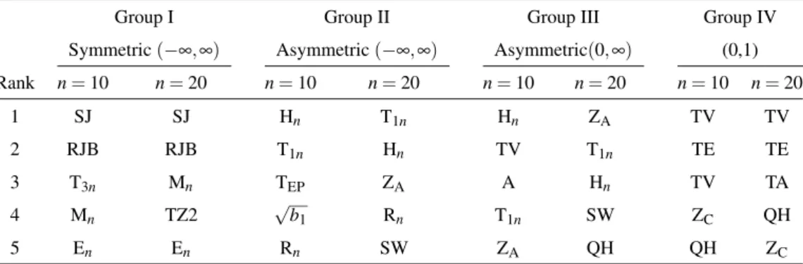
Table 10: Ranking from first to the fifth of average powers computed from values in Tables 6-7 for Set 1of alternative distributions.
Group I Group II Group III Group IV
Symmetric(−∞,∞) Asymmetric(−∞,∞) Asymmetric(0,∞) (0,1)
Rank n=10 n=20 n=10 n=20 n=10 n=20 n=10 n=20 1 SJ SJ Hn T1n Hn ZA TV TV 2 RJB RJB T1n Hn TV T1n TE TE 3 T3n Mn TEP ZA A Hn TV TA 4 Mn TZ2 √b1 Rn T1n SW ZC QH 5 En En Rn SW ZA QH QH ZC
Table 11: Ranking from first to the fifth of average powers computed from values in Tables 8-9 for Set 2of alternative distributions.
Symmetric Asymmetric
Rank Short tailed Close to Normal Long tailed Short tailed Long tailed n=10 n=20 n=10 n=20 n=10 n=20 n=10 n=20 n=10 n=20 1 TV TV Mn RJB SJ SJ Hn Hn T1n T1n 2 TA TA SJ Mn RJB RJB TA TV SW SW 3 SW Rn RJB SJ A2 SF TV TA Rn Rn 4 Hn SW SF SF SF A2 SW SW Hn TA 5 A2 A2 SW T 3n T3n Mn Rn Rn TA Hn
Tables 10-11 contain the ranking from first to the fifth of the average powers com-puted from the values in Tables 6-7 and 8-9, respectively. By average powers we can select the tests that are, on average, most powerful against the alternatives from the given groups.
Power against an alternative distribution has been estimated by the relative frequency of values of the corresponding statistic in the critical region for 10000 simulated sam-ples of size n = 10, 20. The maximum reached power is indicated in bold. For computing the estimated powers of the new test, R software is used. We also use R software for computing Pearson chi-square and Shapiro-Francia tests by the package (nortest),
com-mandpearson.testandsf.test, respectively, and also the package (lawstat),
com-mandsj.testandrjb.testfor SJ and Robast Jarque-Bera tests, respectively. For the
entropy-based test statistics, powers are taken from Zamanzadeh and Arghami (2012) and Alizadeh and Arghami (2011, 2013). In the case of the test based on Hn, we also considerh2(x):=xlog(x)−x+1 for comparison withh1(x):= xx−+11
2 .
Results and recommendations
Based on these comparisons, the following recommendations can be formulated for the application of the evaluated statistics for testing normality in practice.
Set 1of alternative distributions(Tables 6-7 and 10): In Group I, forn=10 and 20, it is seen that the tests based on SJ, RJB, T3n, TZ2, Mnand Enare the most powerful whereas the tests based on In, TV, TC and KL are the least powerful. The difference of powers between KL and the others is substantial. In Group II, forn=10 and 20, it is seen that the tests based on Hn, T1n, TEP, Rn, ZA and√b1 are the most powerful whereas those based on T2n, TV, TC, Kl and Zw are the least powerful. In Group III, the most powerful tests for n=10 are those based on Hn, TV, TA and T1n, and for n=20, those based on ZA, T1n, Hnand SW are the most powerful. On the other hand, the least powerful tests are those based on Inand Zw are the least powerful. Finally, in group IV, the results are not in favour of the proposed tests. In this group, forn=10 and 20, the most powerful tests are those based on TV, TE, TA, ZC, ZA and r, whereas the tests based on TZ2, SJ and RJB are the least powerful. The SJ and RJB show very poor sensitivity against symmetric distributions in[0,1]such as Unif,B(2,2)orB(.5, .5). For example, forn=20, in the case of the [0,1]-Unif alternative, the SJ test has a power of.002 while even the Hn test has a power of .156. From Tables 6-7 one can see that the proportion of times that the SJ and RJB statistics lie below the 5% point of the null distribution are greater than those of the Hnstatistic.
Note that for the proposed test, the maximum power in Group II and III was typically attained by choosingh1.
From the simulation study implemented forSet 1of alternative distributions we can lead to different conclusions from that existing in the literature. New and existing results are reported in Table 12.
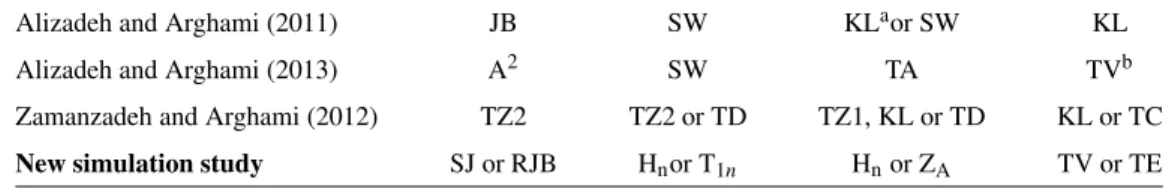
Table 12: Comparison of most powerful tests in Groups I–IV, according to
Alizadeh and Arghami (2011, 2013) and Zamanzade and Arghami (2012) with new simulation results.
Alizadeh and Arghami (2011) JB SW KLaor SW KL
Alizadeh and Arghami (2013) A2 SW TA TVb
Zamanzadeh and Arghami (2012) TZ2 TZ2 or TD TZ1, KL or TD KL or TC New simulation study SJ or RJB Hnor T1n Hnor ZA TV or TE
aStatistic based on Vasicek’s estimator
bStatistic using nonparametric distribution of Vasicek’s estimato
Set 2of alternative distributions(Tables 8-9 and 11): For symmetric short-tailed distributions, it is seen that the tests based on TV, TA and SW are the most powerful. For symmetric close to normal and symmetric long tailed distributions, RJB, JB and Mn are the most powerful. For asymmetric short tailed distributions, Hn, TV and TA are the