Département des Sciences Économiques
de l'Université catholique de Louvain
Multivariate Mixed Normal
Conditional Heteroskedasticity
L. Bauwens, C.M. Hafner and J. Rombouts
CORE DISCUSSION PAPER 2006/12
MULTIVARIATE MIXED NORMAL CONDITIONAL HETEROSKEDASTICITY L. Bauwens1, C.M. Hafner2and J.V.K. Rombouts3
February 20, 2006
Abstract
We propose a new multivariate volatility model where the conditional distribution of a vector time series is given by a mixture of multivariate normal distributions. Each of these distributions is allowed to have a time-varying covariance matrix. The process can be globally covariance-stationary even though some components are not covariance-stationary. We derive some theoretical properties of the model such as the unconditional covariance matrix and autocorrelations of squared returns. The complexity of the model requires a powerful estimation algorithm. In a simulation study we compare estimation by maximum likelihood with the EM algorithm and Bayesian estimation with a Gibbs sampler. Finally, we apply the model to daily U.S. stock returns.
Keywords: Multivariate volatility, Finite mixture, EM algorithm, Bayesian inference.
JEL Classification: C11, C22, C52.
1Universit´e catholique de Louvain, CORE and Department of Economics. 2Universit´e catholique de Louvain, Institut de statistique and CORE. 3HEC Montr´eal, CIRANO, CIRPEE and CREF.
Bauwens’s work was supported in part by the European Community’s Human Potential Programme under contract HPRN-CT-2002-00232, MICFINMA and by a FSR grant from UCL. This text presents research results of the Belgian Program on Interuniversity Poles of Attraction initiated by the Belgian State, Prime Minister’s Office, Science Policy Programming. Rombouts’s work was supported by a HEC Montr´eal Fonds de d´emarrage and by the Centre for Research on e-Finance. The scientific responsibility is assumed by the authors.
Correspondence to Jeroen Rombouts at HEC Montr´eal, 3000 chemin de la Cte-Sainte-Catherine, H3T 2A7, Montreal, Canada. Email: [email protected]
1
Introduction
Several authors have argued in favour of adding flexibility to the family of GARCH models by using the idea of mixture models. For example, extending the model of Wong and Li (2000) and Wong and Li (2001), Haas, Mittnik, and Paolella (2004a) propose a mixed normal conditional heteroskedastic model where the conditional distribution of returns is a mixture of normal distributions, each of which has a regime specific conditional variance specified as a GARCH equation. In this way, they avoid the problem of path-dependence of the conditional variance of regime-switching GARCH models outlined by Gray (1996). Other related papers are those of Haas, Mittnik, and Paolella (2004b) and Alexander and Lazar (2004). All these articles deal with a univariate setting.
Multivariate mixture models have been frequently used in an iid context, but not, to the best of our knowledge, for time series models of conditional volatility, in particular multivariate GARCH models. In this paper, we try to fill this gap by extending the univariate model of Haas, Mittnik, and Paolella (2004a) to the multivariate case. Mixing two or more conditionally normal and heteroskedastic components can generate quite complex stochastic behavior, similar to the one often observed in financial time series. For example, it may be that a component is covariance stationary, another is not, but mixing them might again generate a covariance stationary process. It is possible that mixing many components, of which some are non-stationary, produces behavior similar to processes with long memory, but we have not investigated this issue further.
Note that our approach is different from the regime-switching model of Pelletier (2005), where the unobserved state variable follows a Markov chain and where within a regime correlations are constant.
The paper is organized as follows. In Section 2, we define the model and derive its properties. In Section 3, we present the estimation methods. In Section 4, we illustrate the estimation methods on simulated data, and in Section 5, we present an application using daily data for two stocks. Proofs are relegated in an Appendix.
2
The Model
Consider an N-dimensional vector time series {εt, t ∈ N}. A flexible model for the distribution of εt
conditional on the information setFt−1is given by
εt|Ft−1 ∼ f(λ1, . . . , λk, µ1, . . . , µk,Σ1t, . . . ,Σkt) (1) = k X j=1 λjf(εt|µj,Σjt) (2) whereλj >0, j = 1, . . . , k, Pk
j=1λj = 1 andf(εt|µj,Σjt) is a multivariate density with mean vectorµj
and variance-covariance matrix Σjt. Note that λj is the probability of being in state j, characterized
by the density f(εt|µj,Σjt), and λj is constant over time. Similarly, the means of each state density,
on theµj such that the conditional mean ofεtis zero. For example, one such condition is µk =− k−1 X j=1 (λj/λk)µj. (3)
The first two conditional moments ofεtare then be given by
E[εt| Ft−1) = 0 (4) Var[εt| Ft−1] = k X j=1 λjΣjt (5)
The process εtis conditionally heteroskedastic as every Σjt is allowed to depend on the information
set. We model this dependence using multivariate GARCH (MGARCH) specifications. In particular, we assume that Σjt is a function of εt−1 and of Σj,t−1, which can be called a ‘diagonality’ restriction since
the conditional variance of state j depends only on its own past. In principle, any MGARCH model (VEC, BEKK, DCC,..., see Bauwens, Laurent, and Rombouts (2006)) can be used, but we focus here on the VEC model. Each matrix Σjtis a VEC model, such that
hjt= vech(Σjt) (6)
has the dynamic structure
hjt=ωj+Ajηt−1+Bjhj,t−1 (7)
whereωj is a vector ofN∗=N×(N+ 1)/2 parameters,Aj andBj are square matrices of orderN∗, and
ηt= vech(εtε0t). (8)
In words, we havekVEC models with common shocks that are a function ofεt. We can write the model
compactly as ht=ω+Aηt−1+Bht−1, (9) where ht= h1t h2t .. . hkt kN∗×1 ω= ω1 ω2 .. . ωk kN∗×1 A= A1 A2 .. . Ak kN∗×N∗ B= B1 0 · · · 0 0 B2 · · · 0 .. . ... . .. ... 0 0 · · · Bk kN∗×kN∗ .(10)
We refer to the process defined by equations (1)-(10) as the MN-MGARCH(VEC), for mixed normal MGARCH (in VEC version), model.
For later reference, we provide the uncentered conditional second moment ofεt,
E[ηt| Ft−1] = Λ0ht+c (11)
wherec=Pki=1λivech(µiµ0i), and
Λ = λ1IN∗ .. . λkIN∗ kN∗×N∗ (12)
Theorem 1 The process{εt} defined by (1)-(10) is covariance stationary if and only if the eigenvalues
of the matrix
C=AΛ0+B (13)
are smaller than one in modulus. In that case,
h=E[ht] = (IkN∗−C)−1(ω+Ac) (14)
and the unconditional covariance matrix is given by
E[ηt] = Λ0(IkN∗−C)−1(ω+Ac) +c (15)
The crucial matrix to check is thereforeC, written explicitly
C= λ1A1+B1 λ2A1 · · · λkA1 λ1A2 λ2A2+B2 · · · λkA2 .. . . .. λ1Ak · · · λkAk+Bk kN∗×kN∗
We can get results on the fourth moment structure of the model by assuming that the densities of the individual states are spherical. For simplicity we assume that they are Gaussian with mean zero. Some more notation is necessary. Denote by ˜Λ theN∗2×kN∗2 matrix
˜ Λ = ³ λ1IN∗2,· · · , λkIN∗2 ´ .
Furthermore, letPkqbe thekq2×(kq)2permutation matrix such that for anykq×kqmatrixA,PkqvecA=
(vec(A1)0, . . . ,vec(Ak)0)0, whereAj is thej-thq×qmatrix on the block-diagonal ofA.
Theorem 2 For the process defined by (1)-(10), assume thatf(εt|µj,Σjt) =N(0,Σjt). Then a
neces-sary and sufficient condition for finite fourth moments of εtis that the eigenvalues of the matrix
Z= (A⊗A)GNΛ˜PkN∗+B⊗B+B⊗AΛ0+AΛ0⊗B (16)
have modulus smaller than one, where
GN = 2{(DN+⊗DN+)(IN⊗CN N⊗IN)(DN ⊗DN) +IN∗2},
CN N is the commutation matrix,DN the duplication matrix andDN+ its generalized inverse. In that case,
the unconditional fourth moments of εtare given by
vec(Ση) =GNΛ˜PkN∗(IN∗2−Z)−1γ,
where
γ=vec(ωω0+ωh0ΛA0+ωh0B+AΛ0hω0+B0hω0)
and h is given by (14). Moreover, the autocovariance function of ηt, Γ(τ) = E[ηtηt−τ]−E[ηt]E[ηt]0 is
given by
Γ(τ) = Λ0Cτ−1©AΣη+BΣhΛ−C(IkN∗−C)−1ωω0(IkN∗−C)−1Λ
ª
,
3
Estimation
We describe how we perform estimation by the maximum likelihood (ML) method (section 3.1), by the expectation-maximization (EM) algorithm (section 3.2) of Dempster, Laird, and Rubin (1977), and by Bayesian inference (section 3.3). We assume thatT observation vectors yt, for t= 1 toT, are available
for estimation. The link betweenytandεtin (1) is given byεt=yt−E(yt|Ft−1). We suppose for ease of
presentation that the conditional mean is either known or estimated consistently in a first step, so that the residualsεt are available for estimation of the parameters of the MN-MGARCH(VEC) model in the
second step. We denote byε the vector of observations (ε0
1, ε02, . . . , ε0T)0. We do not write explicitly the
observations before t= 1, which are used as initial conditions where they should appear. The complete parameter vector, called Ψ, regroups the parameters λj,µj, and θj forj = 1, . . . , k, whereθj0 is the row
vector containing all the parameters of ωj, Aj and Bj, see equation (7). Thus, Ψ = (µ0, θ0, λ0)0, where
λ0= (λ
1, λ2, . . . , λk),µ0 = (µ01, µ02, . . . , µ0k), andθ0 = (θ10, θ02, . . . , θ0k).
3.1
ML estimation
The log-likelihood ofεfor the MN-MGARCH(VEC) model is given by
L(Ψ;ε) = T X t=1 log k X j=1 λjφ(εt|µj, θj) , (17)
where φ(·|µj, θj) denotes a multivariate normal density with mean µj and variance-covariance matrix
denoted byhjt, see equation (6),hjt being a function ofθj.
Numerical methods are needed to obtain ˆΨ = arg maxL(Ψ;ε). To avoid the problem of label-switching, we impose the identifying restrictions
λ1> λ2> . . . > λk. (18)
Because of these restrictions, we use the FSQP algorithm of Lawrence and Tits (2001) which allows optimisation subject to constraints.
3.2
EM algorithm
In the EM framework, the observed data vectorεis considered as incomplete since we do not know from which component of the mixture each observation is generated. This information is given by the latent variablezt= (zt1, zt2, . . . , ztK)0 where ztk is a dichotomous variable taking the value 1 ifεt comes from
thek-th mixture component, and 0 otherwise. The complete data log-likelihood is given by
Lc(Ψ;ε) = T X t=1 k X j=1 ztj[logλj+ logφj(εt|µj, θj)]. (19)
This simplifies the expression of the log-likelihood in (17) because we do not take the logarithm over the entire sum but a sum of logarithms. Becauseztis not observed, we proceed in two steps.
E-step: Suppose that Ψ is known and equal to Ψ(i). We compute the expectation of the unobserved
valueztj given all the observationsy. This is given by
E(ztj|ε,Ψ(i)) =τtj(ε; Ψ(i)) = λ(ji)φ(εt|µ(ji), θ (i) j ) Pk j=1λ (i) j φ(εt|µ(ji), θ (i) j ) . (20)
Next, we substitute the latter forztk in (19). This yields the observed complete data log-likelihood:
Q(Ψ,Ψ(i);ε) = T X t=1 k X j=1 τtj(ε; Ψ(i)) [logλj+ logφ(εt|µj, θj)]. (21)
M-step: We maximize numerically Q(Ψ,Ψ(i);ε) with respect to Ψ to get updated estimates of the
parameters, denoted by Ψ(i+1). Notice that we have to impose the constraints (18) and (3), so that the
maximization has to be done numerically with respect to all the parameters, including the probabilities. The E-step and M-step are alternated repeatedly until convergence, see McLachlan and Peel (2000) for a detailed description of the application of the EM algorithm to mixture models.
3.3
Bayesian estimation
We introduce for each observation a state variableSt∈ {1,2, . . . , k}that takes the valuejif the
observa-tionεtbelongs to componentj. Notice thatStconveys the same information asztin the EM algorithm.
The vectorS contains the state variables for theT observations. The model specification assumes that the state variables are independent given the group probabilities, and the probability thatStis equal to
j is equal toλj. Thus, the joint density of the states given the parameters is
ϕ(S|λ) = T Y t=1 ϕ(St|λ) = T Y t=1 λSt. (22)
GivenS and Ψ, the joint density ofεis
f(ε|Ψ, S) =
T
Y
t=1
φ(εt|µSt, θSt). (23)
This would be the likelihood function to use if the states were observed. Since they are not, we treatSas a parameter of the model. This technique is called data augmentation, see Tanner and Wong (1987) for more details. Although the augmented model contains more parameters, inference is feasible by making use of Markov chain Monte Carlo (MCMC) methods. In this paper we implement a Gibbs sampling algorithm that allows to sample from the posterior distribution of S and Ψ by sampling from the full conditional posterior densities of subsets of parameters, which are called the blocks of the Gibbs sampler. The joint posterior distribution is given by
ϕ(S, µ, θ, λ|ε)∝ϕ(µ)ϕ(θ)ϕ(λ)
T
Y
t=1
λStφ(εt|µSt, θSt), (24)
whereϕ(µ),ϕ(θ),ϕ(λ) are the corresponding prior densities. Thus we assume prior independence between
λ, µ and θ. We define these prior densities below while we explain the different blocks of the Gibbs sampler.
3.3.1 Sampling S from ϕ(S|µ, θ, λ, ε)
Given µ, θ, λand ε, the posterior density ofS is proportional to ϕ(S|λ)f(ε|Ψ, S). It turns out that the
St’s are mutually independent, so that we can write the relevant conditional posterior density as
ϕ(S|µ, θ, λ, ε) =
T
Y
t=1
ϕ(St|µ, θ, λ, ε), (25)
whereϕ(St|µ, θ, λ, ε) is a discrete distribution explicitly defined as
P(St=j|µ, θ, λ, ε) = Pkλjφ(εt|µj, θj) i=1λjφ(εt|µj, θj)
, (j= 1, . . . , k). (26) To sampleStwe draw a random number from a uniform distribution on (0,1) and decide which groupj
to take according to (26).
3.3.2 Sampling λfrom ϕ(λ|ST, µ, θ, ε)
The full conditional posterior density ofλis given by
ϕ(λ|S, ε) =ϕ(λ|S)∝ϕ(λ) k Y j=1 λxj j (27)
where xj is the number of times that St = j. The priorϕ(λ) is chosen to be a Dirichlet distribution,
Di(a10, a20· · ·ak0) with parameter vector a0 = (a10, a20· · ·ak0). As a consequence, ϕ(λ|S, ε) is also a
Dirichlet distribution,Di(a1, a2· · ·ak) withaj =aj0+xj,j= 1,2, . . . , k. Notice that it does not depend
onµandθ. To sample aDi(a1, a2· · ·ak) distribution, we samplekindependent gamma random variables,
Xj ∼G(aj,1), and transform them to (see Wilks (1962))
λj = Xj X1+. . .+Xk j= 1, . . . , k−1 λk = 1−λ1−λ2−. . .−λk−1. 3.3.3 Sampling µfrom ϕ(µ|S, λ, θ, ε) We sample ˜µ0 = (µ0
1, µ02, . . . , µ0k−1) and recover µk by use of (3) since λ is known. The likelihood
contribution to the full conditional posterior density of ˜µ, given in (23), can be shown (see the Appendix) to be proportional to a multivariate normal density with variance-covariance matrixA−1and meanA−1b
defined below. Theorem 3 f(ε|Ψ, S)∝exp£−1 2(˜µ−A−1b)0A(˜µ−A−1b) ¤ , wherep= (k−1)N, A=diag X t∈{St=1} Σ−1t1, . . . , X t∈{St=k−1} Σ−k−11,t +˜λ˜λ0 λ2 k X t∈{St=k} Σ−kt1, (28) denoting ˜λ= (λ1, . . . , λk−1), and b= P t∈{St=1}Σ −1 1t εt−λλ1k P t∈{St=k}Σ −1 ktεt .. . P t∈{St=k−1}Σ −1 k−1,tεt−λλk−k1 P t∈{St=k}Σ −1 ktεt . (29)
The variance-covariance matrix A−1 is not block diagonal because of the restriction (3). From the
proposition, we deduce that ifϕ(˜µ) is either a normal density or is non-informative (i.e. proportional to a constant), thenϕ(µ|S, λ, θ, ε), the full conditional posterior ofµ, is also a normal density.
3.3.4 Sampling θ from ϕ(θ|S, µ, λ, ε)
By assuming prior independence between theθj’s, i.e. ϕ(θ) =
Qk j=1ϕ(θj), it follows that ϕ(θ|S, µ, λ, ε) =ϕ(θ|S, µ, ε) =ϕ(θ1|µ1,eε1)ϕ(θ2|µ2,εe2)· · ·ϕ(θk|µk,εek) (30) whereεej ={ε t|St=j}and ϕ(θj|µj,εej)∝ϕ(θj) Y t∈{St=j} φ(εt|µj, θj). (31)
Since we condition on the state variables, we can simulate each blockθj separately. We do this with the
griddy-Gibbs sampler, see Bauwens, Lubrano, and Richard (1999) for details. Note that lower and upper bounds for each parameter must be selected. The choice of these bounds needs to be fine tuned in order to cover the range of the parameter over which the posterior is relevant. The prior for each individual parameter can be uniform between these bounds.
4
Illustration with simulated data
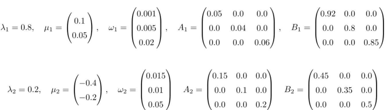
We illustrate the estimation methods on two bivariate two component data generating processes for which we simulate one dataset each. The first one has one stable component with high probability and one unstable component. The parameters are given by
DGP1 λ1= 0.8, µ1= 0.1 0.05 , ω1= 0.001 0.005 0.02 , A1= 0.05 0.0 0.0 0.0 0.04 0.0 0.0 0.0 0.06 , B1= 0.92 0.0 0.0 0.0 0.9 0.0 0.0 0.0 0.85 λ2= 0.2, µ2= −0.4 −0.2 , ω2= 0.015 0.01 0.05 A2= 0.25 0.0 0.0 0.0 0.2 0.0 0.0 0.0 0.3 B2= 0.85 0.0 0.0 0.0 0.75 0.0 0.0 0.0 0.8 .
The largest eigenvalue of the matrixC in (13) is 0.96162 which is smaller than 1 so the overall process is stationary, even if for example A2,11+B2,11 is larger than 1. The implied unconditional standard
deviations for the first and second series are respectively 0.648 and 0.662 and the unconditional correlation is 0.305.
The second DGP has the same first component as DGP1 but the second component is now less per-sistent than the first one. This is done by lowering the values in A2 andB2. The parameters are given
DGP2 λ1= 0.8, µ1= 0.1 0.05 , ω1= 0.001 0.005 0.02 , A1= 0.05 0.0 0.0 0.0 0.04 0.0 0.0 0.0 0.06 , B1= 0.92 0.0 0.0 0.0 0.8 0.0 0.0 0.0 0.85 λ2= 0.2, µ2= −0.4 −0.2 , ω2= 0.015 0.01 0.05 A2= 0.15 0.0 0.0 0.0 0.1 0.0 0.0 0.0 0.2 B2= 0.45 0.0 0.0 0.0 0.35 0.0 0.0 0.0 0.5
The largest eigenvalue of the matrixC in (13) is given by 0.96021 which is smaller than 1 so the overall process is stationary which is not surprising here since both components are stable. The implied un-conditional standard deviations for the first and second series are respectively 0.353 and 0.477 and the unconditional correlation is 0.316.
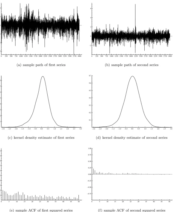
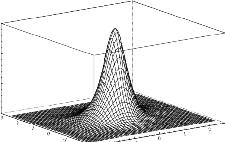
We simulateT = 4000 observations for DGP1 and DGP2. The sample paths, marginal kernel density estimates and sample autocorrelation functions of the data simulated using DGP 1 are given in Figure 1. A bivariate kernel density estimate is given in Figure 2. This estimate is based on a Gaussian product kernel with a scalar bandwidth computed using the rule of thumb. From the graphs we see that the sample autocorrelations for the squared data persist less longer for the second series as we expect given the DGP1 parameter values, and that there is a more negative skewness in the first series than in the second. This is indeed confirmed by the summary statistics given in Table 1. The estimated kurtosis coefficient is higher for the second series, though this is likely due to the high maximum in that series. Note that the empirical second moments match the theoretical second moments reasonably well, for example the estimated and theoretical correlation are respectively given by 0.314 and 0.305.
Table 1: DGP 1 summary statistics
T = 4000
first series second series
Mean 0.0462 0.0416 Standard Deviation 0.5695 0.63826 Maximum 2.5481 6.922 Minimum −3.3493 −3.7382 Skewness −0.45257 −0.03566 Kurtosis 5.298 7.8619
Descriptive statistics of the data simulated using DGP 1. The estimated correlation coefficient is 0.31433.
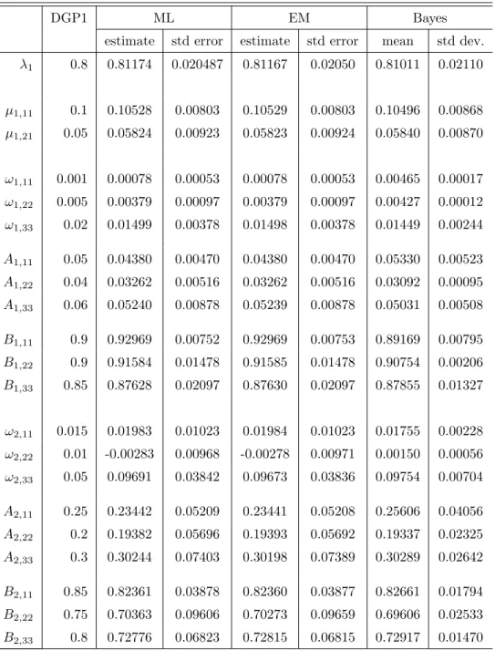
We estimate the parameters of DGP1 using maximum likelihood (ML), the EM algorithm and by Bayesian inference (Bayes), see Section 3 for details. The results are given in Table 2. The ML estimates
0 250 500 750 1000 1250 1500 1750 2000 2250 2500 2750 3000 3250 3500 3750 4000 −3 −2 −1 0 1 2
(a) sample path of first series
0 250 500 750 1000 1250 1500 1750 2000 2250 2500 2750 3000 3250 3500 3750 4000 −2 0 2 4 6
(b) sample path of second series
−3.0 −2.5 −2.0 −1.5 −1.0 −0.5 0.0 0.5 1.0 1.5 2.0 2.5 3.0 0.1 0.2 0.3 0.4 0.5 0.6 0.7 0.8
(c) kernel density estimate of first series
−3.0 −2.5 −2.0 −1.5 −1.0 −0.5 0.0 0.5 1.0 1.5 2.0 2.5 3.0 0.1 0.2 0.3 0.4 0.5 0.6 0.7
(d) kernel density estimate of second series
0 5 10 15 20 25 30 35 40 45 50 0.1 0.2 0.3 0.4 0.5 0.6 0.7 0.8 0.9 1.0
(e) sample ACF of first squared series
0 5 10 15 20 25 30 35 40 45 50 −0.75 −0.50 −0.25 0.00 0.25 0.50 0.75 1.00
(f) sample ACF of second squared series
Figure 1: Sample paths, kernel density estimates and sample autocorrelation functions of the data simu-lated using DGP 1 (4000 observations).
−2 −1 0 1 2 −2 −1 0 1 2 3 0.2 0.4 0.6
Figure 2: kernel density estimate of the data simulated using DGP 1 (4000 observations)
are reasonably close to the true parameter values given the standard errors which are computed via the evaluation of the Hessian at the estimates. Note that the standard errors of the parameters in the second component are drastically higher compared to those of the first component. The likelihood curvature is indeed much smaller for the second component because only 800 = 0.2×4000 observations are expected to come from that component. The EM estimates are almost identical to the ML estimates. The EM standard errors are computed in the same way as for the ML estimates so they also hardly differ. The Bayes’ results are based on 2400 draws of which 400 were discarded to warm up the sampler. Though these results are only indicative in the sense that the marginal posterior standard deviations are too different from the ML standard errors. This is due to too tightly chosen supports, not displayed here, for the parameters drawn using the griddy Gibbs sampler. Therefore, the bounds should be adapted to fully cover the parameter supports. Nevertheless, the posterior standard deviations for the parametersλ1and
µ1 which are sampled with an uninformative prior are reasonably close to their ML standard errors.
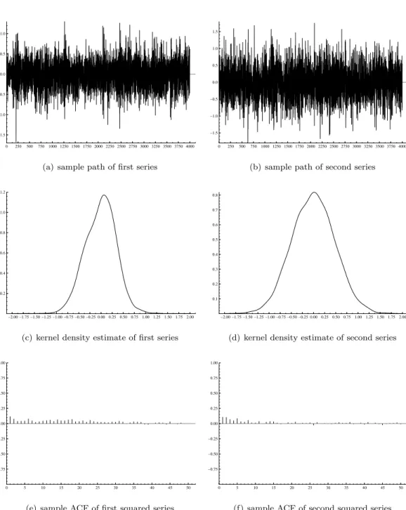
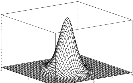
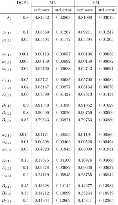
We now turn to DGP2. The sample paths, marginal kernel density estimates and sample autocor-relation functions of the simulated data are given in Figure 3. A bivariate kernel density estimate is given in Figure 4. Descriptive statistics are given in Table 3. The lower autocorrelations in the squared data compared to DGP1 are not surprising given the now much less persistent second component in the mixture. The standard deviations are also smaller compared to DGP1 because we keep the same values in DGP2 for ω1 andω2. Estimation results for DGP2 are given in Table 4. The ML parameter
estimates are again reasonably close to the DGP values. Regarding the EM estimates we find that the parameters of the first component, that is ˆω1,Aˆ1 and ˆB1are very close to the ML estimates. The other
EM parameter estimates, that is ˆλ,µˆ1,ωˆ2,Aˆ2and ˆB2are slightly closer to the true parameter values than
Table 2: DGP1 Two components results
DGP1 ML EM Bayes
estimate std error estimate std error mean std dev.
λ1 0.8 0.81174 0.020487 0.81167 0.02050 0.81011 0.02110 µ1,11 0.1 0.10528 0.00803 0.10529 0.00803 0.10496 0.00868 µ1,21 0.05 0.05824 0.00923 0.05823 0.00924 0.05840 0.00870 ω1,11 0.001 0.00078 0.00053 0.00078 0.00053 0.00465 0.00017 ω1,22 0.005 0.00379 0.00097 0.00379 0.00097 0.00427 0.00012 ω1,33 0.02 0.01499 0.00378 0.01498 0.00378 0.01449 0.00244 A1,11 0.05 0.04380 0.00470 0.04380 0.00470 0.05330 0.00523 A1,22 0.04 0.03262 0.00516 0.03262 0.00516 0.03092 0.00095 A1,33 0.06 0.05240 0.00878 0.05239 0.00878 0.05031 0.00508 B1,11 0.9 0.92969 0.00752 0.92969 0.00753 0.89169 0.00795 B1,22 0.9 0.91584 0.01478 0.91585 0.01478 0.90754 0.00206 B1,33 0.85 0.87628 0.02097 0.87630 0.02097 0.87855 0.01327 ω2,11 0.015 0.01983 0.01023 0.01984 0.01023 0.01755 0.00228 ω2,22 0.01 -0.00283 0.00968 -0.00278 0.00971 0.00150 0.00056 ω2,33 0.05 0.09691 0.03842 0.09673 0.03836 0.09754 0.00704 A2,11 0.25 0.23442 0.05209 0.23441 0.05208 0.25606 0.04056 A2,22 0.2 0.19382 0.05696 0.19393 0.05692 0.19337 0.02325 A2,33 0.3 0.30244 0.07403 0.30198 0.07389 0.30289 0.02642 B2,11 0.85 0.82361 0.03878 0.82360 0.03877 0.82661 0.01794 B2,22 0.75 0.70363 0.09606 0.70273 0.09659 0.69606 0.02533 B2,33 0.8 0.72776 0.06823 0.72815 0.06815 0.72917 0.01470
0 250 500 750 1000 1250 1500 1750 2000 2250 2500 2750 3000 3250 3500 3750 4000 −1.5 −1.0 −0.5 0.0 0.5 1.0
(a) sample path of first series
0 250 500 750 1000 1250 1500 1750 2000 2250 2500 2750 3000 3250 3500 3750 4000 −1.5 −1.0 −0.5 0.0 0.5 1.0 1.5
(b) sample path of second series
−2.00 −1.75 −1.50 −1.25 −1.00 −0.75 −0.50 −0.25 0.000.25 0.50 0.75 1.00 1.251.50 1.75 2.00 0.2 0.4 0.6 0.8 1.0 1.2
(c) kernel density estimate of first series
−2.00 −1.75 −1.50 −1.25 −1.00 −0.75 −0.50 −0.25 0.000.25 0.50 0.751.00 1.25 1.50 1.75 2.00 0.1 0.2 0.3 0.4 0.5 0.6 0.7 0.8
(d) kernel density estimate of second series
0 5 10 15 20 25 30 35 40 45 50 −0.75 −0.50 −0.25 0.00 0.25 0.50 0.75 1.00
(e) sample ACF of first squared series
0 5 10 15 20 25 30 35 40 45 50 −0.75 −0.50 −0.25 0.00 0.25 0.50 0.75 1.00
(f) sample ACF of second squared series
Figure 3: Sample paths, kernel density estimates and sample autocorrelation functions of the data simu-lated using DGP 2 (4000 observations).
−1 0 1 2 −1 0 1 2 0.25 0.50 0.75
Figure 4: kernel density estimate of the data simulated using DGP 1 (4000 observations)
Table 3: DGP 2 summary statistics
T = 4000
first series second series
Mean −0.01015 −0.00514 Standard Deviation 0.34385 0.48067 Maximum 1.2971 1.7524 Minimum −1.6771 −1.7772 Skewness −0.12201 0.01965 Kurtosis 3.2058 3.0245
Descriptive statistics of the data simulated using DGP 2. The estimated correlation coefficient is 0.32746.
Table 4: DGP2 Two components results
DGP2 ML EM
estimate std error estimate std error
λ1 0.8 0.81942 0.02863 0.81080 0.03019 µ1,11 0.1 0.08860 0.01207 0.09211 0.01247 µ1,21 0.05 0.05404 0.01172 0.05394 0.01203 ω1,11 0.001 0.00113 0.00057 0.00106 0.00056 ω1,22 0.005 0.00159 0.00082 0.00159 0.00082 ω1,33 0.02 0.02760 0.00688 0.02743 0.00691 A1,11 0.05 0.05721 0.00685 0.05700 0.00682 A1,22 0.04 0.03147 0.00877 0.03134 0.00876 A1,33 0.06 0.07890 0.01427 0.07813 0.01434 B1,11 0.9 0.91040 0.01030 0.91052 0.01029 B1,22 0.8 0.90690 0.03026 0.90759 0.03000 B1,33 0.85 0.79543 0.03871 0.79753 0.03880 ω2,11 0.015 0.01171 0.00555 0.01191 0.00560 ω2,22 0.01 0.00398 0.00462 0.00526 0.00494 ω2,33 0.05 0.04923 0.01948 0.05009 0.01931 A2,11 0.15 0.17075 0.04100 0.16976 0.04060 A2,22 0.1 0.09478 0.03682 0.09636 0.03637 A2,33 0.2 0.24119 0.05945 0.23755 0.05842 B2,11 0.45 0.43228 0.14142 0.44277 0.13984 B2,22 0.35 0.34712 0.19099 0.35254 0.18539 B2,33 0.5 0.44934 0.12669 0.45841 0.12265
To be sure that the results are correct, we generate some extra sample paths for both DGP1 and DGP2 of the same sample size and then we estimate the model parameters again, the results of which are not reported here. It follows that the conclusions are the same as described above in this section.
5
Application
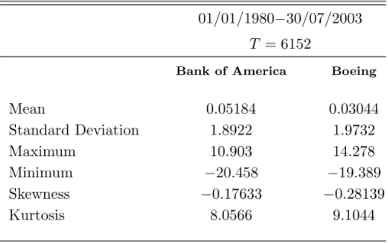
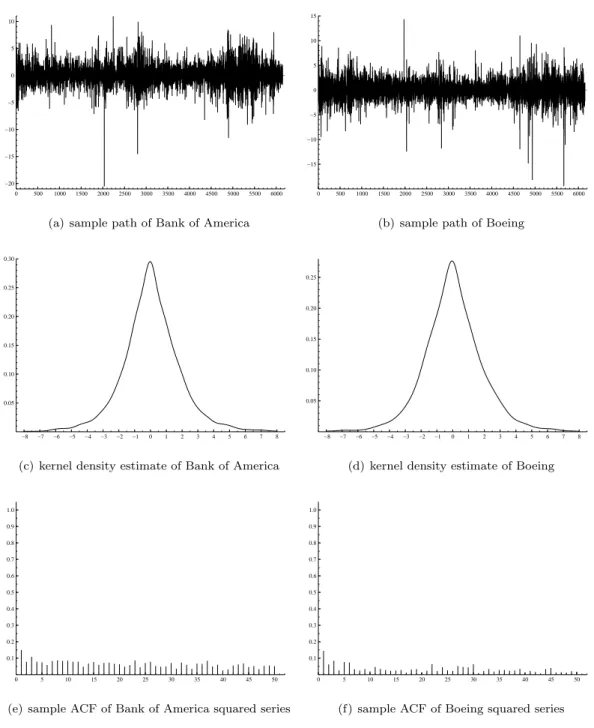
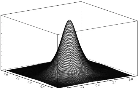
We model daily return data from the Bank of America and Boeing stocks using a sample from 01/01/1980 to 30/07/2003 implying 6152 observations downloaded from Datastream. Daily returns are measured by log-differences of closing prices. The sample paths, marginal kernel density estimates and sample autocorrelation functions of the data are given in Figure 5. A bivariate kernel density estimate is given in Figure 6. Both companies share similar summary statistics which are given in Table 5. Some important events between 1980 and 2003 give rise to several extreme values for both companies. These values are not discarded from the sample. We start by fitting univariate one and two component models to learn
Table 5: Bank of America - Boeing summary statistics 01/01/1980−30/07/2003
T = 6152
Bank of America Boeing
Mean 0.05184 0.03044 Standard Deviation 1.8922 1.9732 Maximum 10.903 14.278 Minimum −20.458 −19.389 Skewness −0.17633 −0.28139 Kurtosis 8.0566 9.1044
Descriptive statistics for the Bank of America - Boeing data. The estimated correlation coefficient is 0.25448.
more about the individual time series dynamics of both companies and also to get an idea of good starting values for the multivariate mixture model. The ML estimates for the univariate models are displayed in Table 6. We can also apply Bayesian inference or the EM algorithm but the results are very similar to the ML estimates and are not reported. The one component model, or the usual GARCH model, estimates for both Bank of America and Boeing imply stationary but highly persistent processes. The two component mixture model parameter estimates reveal indeed that for both companies the second component is not stable with probabilities belonging to that component respectively given by 0.165 and 0.079.
The estimation results for the bivariate one and two component models are given in Table 7. The largest eigenvalue of the estimated matrix C in (13) is given by 0.98435 which implies a stationary process. The implied estimated unconditional standard deviations for Bank of America and Boeing are
0 500 1000 1500 2000 2500 3000 3500 4000 4500 5000 5500 6000 −20 −15 −10 −5 0 5 10
(a) sample path of Bank of America
0 500 1000 1500 2000 2500 3000 3500 4000 4500 5000 5500 6000 −15 −10 −5 0 5 10 15
(b) sample path of Boeing
−8 −7 −6 −5 −4 −3 −2 −1 0 1 2 3 4 5 6 7 8 0.05 0.10 0.15 0.20 0.25 0.30
(c) kernel density estimate of Bank of America
−8 −7 −6 −5 −4 −3 −2 −1 0 1 2 3 4 5 6 7 8 0.05 0.10 0.15 0.20 0.25
(d) kernel density estimate of Boeing
0 5 10 15 20 25 30 35 40 45 50 0.1 0.2 0.3 0.4 0.5 0.6 0.7 0.8 0.9 1.0
(e) sample ACF of Bank of America squared series
0 5 10 15 20 25 30 35 40 45 50 0.1 0.2 0.3 0.4 0.5 0.6 0.7 0.8 0.9 1.0
(f) sample ACF of Boeing squared series
Figure 5: Sample paths, kernel density estimates and sample autocorrelation functions for the Bank of America - Boeing data
−5.0 −2.5 0.0 2.5 5.0 −5.0 −2.5 0.0 2.5 5.0 0.025 0.050 0.075
Figure 6: kernel density estimate for the Bank of America - Boeing data
Table 6: Univariate estimation results
Bank of America Boeing
estimate std error estimate std error estimate std error estimate std error
λ1 - - 0.83546 0.02812 - - 0.92084 0.01597 µ1 - - 0.02161 0.01960 - - -0.00607 0.01678 ω1 0.13539 0.02952 0.03144 0.01298 0.05496 0.00172 0.02882 0.00879 A1,11 0.08175 0.01214 0.04652 0.00925 0.04009 0.00927 0.03010 0.00476 B1,11 0.88053 0.01901 0.91757 0.01721 0.94618 0.01640 0.94770 0.00859 ω2 - - 3.1304 0.94430 - - 2.6525 1.2180 A2,11 - - 0.69763 0.18304 - - 0.51102 0.20203 A2,11 - - 0.41636 0.12488 - - 0.73011 0.09004
Results for the one component (first two columns for each company) and two component (last two columns for each company) univariate mixture GARCH(1,1) models. All the parameters are estimated by ML.
respectively given by 1.8653 and 1.9716 and the unconditional correlation is 0.209, which is close to the summary statistics reported in Table 5. Comparing the univariate one component estimates with their equivalents in the bivariate one component model, or the usual diagonal VEC model, we see that they differ only marginally as expected. Generally speaking, this is also true for the bivariate two component model but to a lesser extent so for the second component which is now stable. The large difference in the loglikelihood function values evaluated at their ML estimates between the one and the two component models allows to reject easily a likelihood ratio test in favor of the more general model.
6
Conclusion
The multivariate mixture model we have proposed in this paper can be extended in several ways. One can use other multivariate GARCH models for the components than the VEC formulation. We refer to the survey of Bauwens, Laurent, and Rombouts (2006) for other multivariate GARCH models. One advantage of the VEC specification is the ease with which moments can be derived. One could also think of using non-normal distributions, but this may not be worth the effort since a mixture of normal distributions allows for a lot of flexibility. The most important challenge at this stage is to improve upon the estimation algorithms (especially the Bayesian one) and to test them with time series of higher dimension. Another topic for future research is to evaluate the models on statistical and economic criteria, in comparison with one-component models.
Appendix
Proof of Theorem 1: Letut=ηt−Λ0ht−cand note that E[ut|It−1] = 0. Write (9) as
ht = ω+A(Λ0ht−1+c+ut−1) +Bht−1
= (ω+Ac) + (AΛ0+B)ht−1+Aut−1
Denoting the lag operator byL andC=AΛ0+B, this can be written as
(IkN∗−CL)ht= (ω+Ac) +Aut−1. (32)
The linear operator (IkN∗−CL) is invertible if and only if all eigenvalues ofChave modulus smaller than
one. In that case we can writeht= (IkN∗−C)−1(ω+Ac) + (IkN∗−CL)−1Aut−1, which is a VMA(∞)
representation of{ht}from which we directly deduceh= E[ht] = (IkN∗−C)−1(ω+Ac). Premultiplying
both sides of (32) by the adjoint, (IkN∗−CL)∗, we obtain
det(IkN∗−CL)ht= (IkN∗−C)∗(ω+Ac) + (IkN∗−CL)∗Aut−1
Premultiplying by Λ0 and using Λ0h
t=ηt−ut−c gives
Table 7: Bank of America - Boeing results
ML EM
estimate std error estimate std error estimate std error
λ1 - - 0.85592 0.01889 0.84833 0.01954 µ1,11 - - 0.03675 0.01771 0.03720 0.01801 µ1,21 - - -0.01075 0.01907 -0.01290 0.01937 ω1,11 0.14562 0.02857 0.03041 0.00996 0.02957 0.00986 ω1,22 0.02617 0.00753 0.00372 0.00159 0.00365 0.00158 ω1,33 0.07300 0.01677 0.02810 0.00880 0.02768 0.00879 A1,11 0.08353 0.01124 0.04588 0.00754 0.04536 0.00746 A1,22 0.02587 0.00506 0.01146 0.00270 0.01137 0.00266 A1,33 0.04122 0.00535 0.02748 0.00439 0.02730 0.00441 B1,11 0.87564 0.01786 0.92578 0.01243 0.92609 0.01244 B1,22 0.93974 0.01312 0.97453 0.0052841 0.97451 0.00528 B1,33 0.94011 0.00891 0.94771 0.0088205 0.94761 0.00894 ω2,11 - - 3.5169 1.0715 3.3482 0.95338 ω2,22 - - 0.41860 0.29750 0.41166 0.27223 ω2,33 - - 2.2500 0.83084 2.1491 0.77734 A2,11 - - 0.60068 0.15838 0.58961 0.15030 A2,22 - - 0.13174 0.07384 0.12842 0.06905 A2,33 - - 0.25788 0.08024 0.25432 0.07685 B2,11 - - 0.36883 0.14227 0.38091 0.12996 B2,22 - - 0.78676 0.12018 0.78481 0.11659 B2,33 - - 0.72074 0.07796 0.72330 0.07600
Results for the one component (first two columns) and two component (last four columns) bivariate mixture model. The value of the loglikelihood function evaluated at the ML es-timates of the one and two component models are respectively given by −24663.714 and
The process is stable if and only if all roots of the characteristic equation det(IkN∗−Cz) = 0 lie outside
the unit circle or, equivalently, all eigenvalues ofChave modulus smaller than one. Finally, dividing both sides by det(IkN∗−CL) and rearranging yields
ηt= Λ0(IkN∗−C)−1(ω+Ac) +c+ Λ0(IkN∗−CL)−1Aut−1+ut
This is the VMA(∞) representation of {ηt} and we deduce directly the unconditional variance of{εt},
i.e.
vech(Var(εt)) = E[ηt] = Λ0(IkN∗−C)−1(ω+Ac) +c
Proof of Theorem 2: First, vec(E[ηtηt0 | Ft−1]) =GN
Pk
j=1λjvec(hjth0jt) by application of Theorem 1
of Hafner (2003). Taking the expectation operator on both sides yields
vec(Ση) =GNΛ˜PkN∗vec(Σh) (33)
where Ση= E[ηtη0t] and Σh= E[hth0t]. Substituting the model forhtin Σh, one obtains
vec(Σh) = vec(ωω0+ωh0ΛA0+ωh0B+AΛ0hω0+B0hω0) + (A⊗A)vec(E[ηt−1ηt−0 1]) + (B⊗B)vec(E[ht−1h0t−1]) + (B⊗A)vec(E[ηt−1h0t−1]) + (A⊗B)vec(E[ht−1ηt−1]) = γ+ (A⊗A)vec(Ση) + (B⊗B)vec(Σh) + (B⊗A)vec(E[E(ηt−1h0t−1| Ft−1)]) + (A⊗B)vec(E[E(ht−1ηt−1| Ft−1)]) = γ+ (A⊗A)GNΛ˜PkN∗vec(Σh) + (B⊗B)vec(Σh) + (B⊗A)vec(E[Λ0h t−1h0t−1]) + (A⊗B)vec(E[ht−1h0t−1Λ])
= γ+ (A⊗A)GNΛ˜PkN∗vec(Σh) + (B⊗B)vec(Σh) + (B⊗AΛ0)vec(Σh) + (AΛ0⊗B)vec(Σh)
= γ+Zvec(Σh).
Rearranging gives the result provided that IN∗2 −Z is invertible, which is the case if and only if all
eigenvalues ofZ have modulus smaller than one. Finally, application of (33) yields the desired result for Ση.
For the second part of the theorem, note that
E[ht| Ft−τ] = (IkN∗+C+· · ·+Cτ−1)ω+Cτ−1(Aηt−τ+Bht−τ) = (IkN∗−Cτ)(IkN∗−C)−1ω+Cτ−1(Aηt−τ+Bht−τ) Now, E[ηtηt−τ] = E[E(ηt| Ft−1)ηt−τ0 ] = E[Λ0h tηt−τ0 ] = E[Λ0E(ht| Ft−τ)η0t−τ] = E[Λ0{(I kN∗−Cτ)(IkN∗−C)−1ω+Cτ−1(Aηt−τ+Bht−τ)}ηt−τ0 ]
= Λ0(I
kN∗−Cτ)(IkN∗−C)−1ωω0(IkN∗−C0)−1Λ + Λ0Cτ−1(AΣη+BΣhΛ)
Subtracting E[ηt]E[ηt]0= Λ0{(IkN∗−C)−1ωω0(IkN∗−C0)−1Λ, the result for Γ(τ) is obtained.
Proof of Theorem 3: We start from (23), where we substitute−Pk−j=11(λj/λk)µjforµk and we neglect
all the factors that do not depend on ˜µ. Given the state variables, we know to which group each observation εt belongs and we denote by {St = j} the set of indices of the observations belonging to
groupj. Thus, taking the logarithm of (23) and multiplying it by−2, we get
−2 T X t=1 logφ(εt|µSt, θSt)−C = −2 k X j=1 X t∈{St=j} logφ(εt|µj, θj)−C = k−X1 j=1 X t∈{St=j} (εt−µj)0Σjt−1(εt−µj) + X t∈{St=k} µ εt+ ( k−1 X j=1 λj λjµj) ¶0 Σ−jt1 µ εt+ ( k−1 X j=1 λj λjµj) ¶ = k−X1 j=1 X t∈{St=j} · Cj+µ0j µ X t∈{St=j} Σ−jt1 ¶ µj−2µ0j µ X t∈{St=j} Σ−jt1εt ¶¸ + X t∈{St=k} · Ck+ µk−X1 j=1 λj λkµj ¶0µ X t∈{St=k} Σ−1 kt ¶µk−X1 j=1 λj λkµj ¶ + 2 µk−X1 j=1 λj λkµj ¶0µ X t∈{St=k} Σ−1 ktεt ¶¸ = k−X1 j=1 · µ0 j µ X t∈{St=j} Σ−1 jt + λ2 j λ2 k X t∈{St=k} Σ−1 kt ¶ µj ¸ + k−1 X j=1 X i6=j µ0 j ·µ λjλi λ2 k X t∈{St=k} Σ−1 kt ¶ µi ¸ −2 k−1 X j=1 · µ0 j µ X t∈{St=j} Σ−1 jt εt−λj λk X t∈{St=k} Σ−1 ktεt ¶¸ + k X j=1 Cj = ˜µ0Aµ˜−2˜µ0b+ k X j=1 Cj = (˜µ−A−1b)0A(˜µ−A−1b) + k X j=1 Cj−b0A−1b
whereCand theCj’s are constants that do not depend on ˜µ, whileAandbare defined in (28) and (29).
Therefore, by taking the exponential of minus one half of the the last expression, and neglecting the two irrelevant constant terms, we get
exp−1
2(˜µ−A
−1b)0A(˜µ−A−1b), (34)
which is the kernel of aNp(A−1b, A−1) density for ˜µ.
References
Alexander, C., and E. Lazar (2004): “Normal Mixture GARCH(1,1),” forthcoming in Journal of Applied Econometrics.
Bauwens, L., S. Laurent, and J. Rombouts(2006): “Multivariate GARCH Models: A Survey,” Journal of Applied Econometrics, 21, forthcoming.
Bauwens, L., M. Lubrano, and J. Richard (1999): Bayesian Inference in Dynamic Econometric Models. Oxford University Press, Oxford.
Dempster, A., N. Laird, and D. Rubin(1977): “Maximimum Likelihood From Incomplete Data via the EM Algorithm (with discussion),”Journal of the Royal Statistical Society, Ser. B, 39, 1–38.
Gray, S.(1996): “Modeling the conditional distribution of interest rates as a regime-switching process,” Journal of Financial Economics, 42, 27–62.
Haas, M., S. Mittnik, and M. Paolella (2004a): “Mixed Normal Conditional Heteroskedasticity,” Journal of Financial Econometrics, 2, 211–250.
(2004b): “A New Approach to Markov-Switching GARCH Models,”Journal of Financial Econo-metrics, 2, 493–530.
Hafner, C.(2003): “Fourth Moment Structure of Multivariate GARCH processes,”Journal of Financial Econometrics, 1, 26–54.
Lawrence, C., andA. Tits(2001): “A Computationally Efficient Feasible Sequential Quadratic Pro-gramming Algorithm,”SIAM Journal of Optimization, 11, 1092–1118.
McLachlan, G., and D. Peel(2000): Finite Mixture Models. Wiley Interscience, New York.
Pelletier, D. (2005): “Regime Switching for Dynamic Correlations,” forthcoming in the Journal of Econometrics.
Tanner, M., and W. Wong(1987): “The Calculation of Posterior Distributions by Data Augmenta-tion,”Journal of the American Statistical Association, 82, 528–540.
Wilks, S.(1962): Mathematical Statistics. Wiley, New York.
Wong, C., and W. Li(2000): “On a Mixture Autoregressive Model,” Journal of the Royal Statistical Society, Series B, 62, 95–115.
(2001): “On a Mixture Autoregressive Conditional Heteroscedastic Model,” Journal of the American Statistical Association, 96, 982–995s.