Numerical Simulation of Flow over an Airfoil with a Cavity
W. F. J. Olsman
∗Eindhoven University of Technology, 5600 MB Eindhoven, The Netherlands
and
T. Colonius
†California Institute of Technology, Pasadena, California 91125
DOI: 10.2514/1.J050542Two-dimensional direct numerical simulation of theflow over a NACA0018 airfoil with a cavity is presented. The low Reynolds number simulations are validated by means offlow visualizations carried out in a water channel. From the simulations, it follows that there are two main regimes offlow inside the cavity. Depending on the angle of attack, thefirst or the second shear-layer mode (Rossiter tone) is present. The global effect of the cavity on theflow around the airfoil is the generation of vortices that reduceflow separation downstream of the cavity. At high positive angles of attack, theflow separates in front of the cavity, and the separatedflow interacts with the cavity, causing the generation of smaller-scale structures and a narrower wake compared with the case when no cavity is present. At certain angles of attack, the numerical results suggest the possibility of a higher lift-to-drag ratio for the airfoil with cavity compared with the airfoil without cavity.
Nomenclature
c = chord of airfoil, mD = cavity depth, m
f = frequency, Hz
k = reduced frequency
Rec = Reynolds number based on chord length Sth = Strouhal number based on projected frontal area StW = Strouhal number based on cavity opening U1 = freestream velocity,m=s
W = cavity opening, m
= angle of attack,
= kinematic viscosity,m2=s
= boundary-layer momentum thickness, m
! = oscillation frequency,rad=s
I.
Introduction
R
ECENTLY, the Kasper vortex wing concept has received new attention. The Kasper wing was claimed to achieve higher lift-to-drag ratios compared with conventional airfoils (see [1] and references therein). This high ratio was argued to be caused by trapping a vortex (or multiple vortices) in the vicinity of the airfoil at all times. A potential advantage of such a wing is that it can be relatively thick, which is useful from a structural point of view for applications such as high-altitude long endurance (HALE) aircraft or wind turbines. The current work has been performed within a project considering HALE application.‡After the original claim of Kasper of high lift-to-drag ratio and trapped vortices, scale models of the Kasper vortex lift wing were tested in a wind tunnel [1]. None of the tested configurations of the vortex wing performed as well as a conventional airfoil. It was suggested that the discrepancy between the wind-tunnel experiments and the claimedflow with trapped vortices was due to the Reynolds number being too low during the wind-tunnel tests.
Although the original claim by Kasper was not supported by the wind-tunnel experiment, theoretical studies have shown that airfoils with trapped vortices can have favorable properties, such as high lift-to-drag ratio or prevention of periodic vortex shedding at high angles of attack. It was recently shown that, in a potentialflow with two trapped vortices, a nonzero volume body with lift exists with a favorable pressure gradient along the entire contour of the body [2]. A favorable pressure gradient is beneficial, because it preventsflow separation.
Construction of a solution of theflow past an airfoil with a cavity and a trapped vortex is provided by Bunyakin et al. [3,4]. In both papers, theflow is a Batchelor-modelflow, which means that theflow is steady, two-dimensional, and the vorticity is uniform inside the region of closed streamlines and zero outside, corresponding to the high Reynolds number limit.
Rectangular cavities in plane walls have been studied extensively [5]. However, not much literature is available for the case of a cavity placed in an airfoil. From the literature about cavities in plane walls, it is known that a cavity can display a shear-layer instability mode that oscillates at a Strouhal number, StWfW=U1, of order unity, whereW is the width of the cavity opening,f is the oscillation frequency, andU1is the freestream velocity [6]. The cavity may also give rise to a cavity wake mode [7], although this mode is rarely observed in planar geometries. In the literature, cavities can be classified as either deep or shallow, depending on the ratio of cavity depthDto cavity openingW. Furthermore, one distinguishes for very shallow cavities between open and closed cavities, depending on the reattachment of theflow on the wall within the cavity. For the cavity considered in this paper,D=WO1, which corresponds to an open, shallow cavity.
Because of the approximations made in the theory for designing a wing with a cavity, some of the features of a cavity are omitted, such as the oscillations of the shear layer. The oscillations of the shear layer above the cavity might have a considerable effect on the aero-dynamic characteristics of the airfoil in steady as well as unsteady
flow. In the case where the opening of the cavity is a significant portion of the chord length of the airfoil, the oscillations of the shear layer might interfere with the shedding of vorticity at the trailing edge. In the current paper, we will focus on the aerodynamics of the airfoil in a steady uniform freestream.
The available theoretical studies mainly focus on approximate theory (inviscid or Bachelor-modelflow). In the current paper, we attempt to gain more insight into theflow physics by means of two-dimensional direct numerical simulation (DNS) of the Received 11 March 2010; revision received 5 August 2010; accepted for
publication 7 September 2010. Copyright © 2010 by the American Institute of Aeronautics and Astronautics, Inc. All rights reserved. Copies of this paper may be made for personal or internal use, on condition that the copier pay the $10.00 per-copy fee to the Copyright Clearance Center, Inc., 222 Rosewood Drive, Danvers, MA 01923; include the code 0001-1452/11 and $10.00 in correspondence with the CCC.
∗Ph.D. Student, Department of Physics; [email protected].
†Professor, Department of Mechanical Engineering. Associate Fellow
AIAA. ‡Data available at www.vortexcell2050.org [retrieved 14 October 2010].
Vol. 49, No. 1, January 2011
incompressible Navier–Stokes equations. Because of the separated nature of the flow and instabilities, Reynolds-averaged Navier– Stokes computations are not expected to correctly predict theflow. A three-dimensional large eddy simulation (LES) would be expected to capture theflow physics but would be very expensive. Therefore, a preliminary numerical solution would be a two-dimensional DNS. The simulations are qualitatively validated byflow visualizations in a water channel.
In this paper, we will use a geometry that was designed for quick manufacture and low cost. First, the numerical model used will be briefly discussed. Then the results of the numerical simulations for a standard airfoil are presented and compared with experimental data from literature. Hereafter, the computations of theflow around the airfoil with a cavity will be compared withflow visualizations in a water channel and with the numerical results of the standard airfoil.
II.
Numerical Method
The two-dimensional incompressible Navier–Stokes equations are solved using an immersed boundary (IB) projection method [8,9]. The solid body of the airfoil is represented, on a regular Cartesian grid, by a set of discrete forces that are in turn regularized (smeared) on the grid. At these discrete body points, the no-slip condition is exactly enforced. The equations are discretized with a second-order
finite volume method, and a streamfunction-vorticity approach is used on a staggered grid arrangement. Because of the streamfunction approach, the divergence-free constraint is exactly satisfied (to machine precision). The IB treatment gives rise to afirst-order error in the momentum equations near the surface of the body; empirical convergence studies [8] show better thanfirst-order accuracy in the L2 norm. Further details regarding the numerical method can be found in the aforementioned references.
Numerical simulations are performed for several angles of attack , measured in degrees. The angle of attack is defined positive, as indicated in Fig. 1. The standard NACA0018 airfoil is described by 2779 points on its surface, at which the no-slip condition is enforced. For the airfoil with a cavity, this is 2995 points. The properties of the calculations for a positive angle of attack are listed in Table 1. For the airfoil with a cavity, the same cases as listed in Table 1 are also run with the same properties at the corresponding negative angles of attack. The computational domain typically extends to a distance of 12 chord lengths in the upstream and downstream directions and three chord lengths in the upper and lower normal directions. Our IB method uses a series of overlapping consecutively larger and coarser grids; the number of grids is listed in Table 1 as grid levels. The smallest domain with the finest resolution extends to 1.5 chord lengths in the streamwise and 0.35 in the normal directions. The nondimensional grid spacing=con thisfinest grid is7:4104for
the majority of cases studied. Selected cases are run on a coarser grid with =c1:1103 to test grid convergence. The standard
NACA0018 airfoil is computed at four angles of attack: 0, 4, 10, and 15. The computational settings are the same as those listed for the airfoil with a cavity. Typical run times are in the order of 700 h on a single Advance Micro Devices, Inc. Opteron processor.
In the IB method, the discrete points at which the no-slip condition is enforced cannot be too close to each other. Typically, the distance between those points needs to be equal to or slightly greater than the grid spacing. Note that if the distance between the points is too large, then the surface is porous. At the sharp trailing edge, points of the upper and lower surfaces can be too close to each other. This issue is dealt with by omitting a few points on either the upper or lower surfaces. The standard NACA0018 airfoil without a cavity at a zero
angle of attack is also computed with a rounded trailing edge where no points are omitted. The trailing-edge radius is 0.3% of the chord length, which is the same as that of the experimental airfoil. The rounded trailing edge is described by approximately 10 points.
For selected cases, grid resolution and domain size were varied, in order to assess convergence and influence of the far-field boundary. From these results, one can conclude that the results presented, with the resolutions and domain sizes indicated in Table 1, are essentially grid independent. It should be noted that theflows considered show signs of chaotic behavior in vortex shedding. The Reynolds number is sufficiently high such that the formation of large-scale vortices and the subsequent pairing of these structures gives rise to aperiodic low-frequency oscillations that are difficult to characterize, because the run times are not sufficiently long to observe many periods. Thus, two cases at slightly different resolutions ultimately become decorre-lated from each other and contain oscillations over sufficiently long times such that it is not possible to distinguish any possible contamination from the far-field boundaries. However, in all cases, we observed that the time-averaged quantities and qualitativeflow regimes are indeed grid independent.
III.
Results
Two-dimensional simulations are preformed for a standard NACA0018 airfoil and a NACA0018 airfoil with a cavity. The NACA0018 airfoil with a cavity is shown in Fig. 1. The cavity mouth hasW=c0:21. Both edges of the cavity are sharp. The forward sharp edge willfix the separation point, and the rear sharp edge will maximize the feedback loop of the shear layer. This configuration is expected to give the most extreme oscillations of the shear layer.
In all the simulations, the Reynolds number based on the chord length isRecU1c=2104, withas the kinematic viscosity of thefluid. In the following sections, the results of the computations will be presented and compared with experimental data from literature andflow visualization performed in a water channel. First, the results for the standard NACA0018 airfoil (clean airfoil) are presented, then the results for the NACA0018 airfoil with a cavity are discussed and compared with the standard NACA0018 airfoil and experimental data.
A. NACA0018
In this section, the results of the numerical simulation of the clean airfoil are presented. At0, theflow initially separates around 50% of the chord length. Literature reports separation at 51% of the chord length from the leading edge forRec1:6105[10]. This separation causes a periodic vortex shedding in the wake of the airfoil. We define, here, the Strouhal numberSthfh=U1, withh as the projected frontal area of the airfoil. At0,his equal to the thickness of the airfoil andSth0:42. As theflow develops, the periodic shedding is modulated by a much lower frequency oscillation. The separation points begin to oscillate upstream and downstream, with opposite phases on the upper and lower surfaces. The entire wake is shifted up and down during this low-frequency cycle while its structure is unchanged. Snapshots of the vorticity contours are shown at minimum and maximum lifts in Figs. 2a and 2b, respectively. For this low-frequency oscillation,Sth1:0102 c
W
α
Fig. 1 NACA0018 airfoil with a cavity, with chord lengthc165mm and cavity opening of W34mm. A probe location used in the numerical simulations is shown by the tilted square.
Table 1 Setting for NACA0018 cases, with and without cavity Angle of attack, Smallest
box size Largest box size Grid levels Total number of cells 0.0 1:490:328 23:95:25 5 4:4106 1.0 1:490:328 23:95:25 5 4:4106 2.0 1:490:328 23:95:25 5 4:4106 3.0 1:490:358 23:95:73 5 4:8106 4.0 1:490:358 23:95:73 5 4:8106 6.0 1:490:358 23:95:73 5 4:8106 10.0 1:490:358 23:95:73 5 4:8106 15.0 1:490:433 47:813:9 6 6:96106
and the amplitude of the lift force caused by this low-frequency oscillation is a factor of four larger than the amplitude of the oscillations due to the periodic vortex shedding. Additional calcul-ations have shown that a lower curvature of the trailing edge causes the amplitude of the low-frequency oscillation to decrease by about 10%, but it does not eliminate it. At0:5, the low-frequency oscillation is also present. A calculation atRec104did not display the low-frequency oscillation. The low-frequency behavior is most likely caused by a unique combination of Reynolds number and geometry. It is likely that this low-frequency behavior is very sensitive to three-dimensional effects and turbulence, which could be a reason why it may not be observed in experiments. There is, however, evidence of similar behavior in literature, but this was reported for airfoils near stall conditions [11].
At4, the separation point on the suction side moves upstream to about 25% of the chord length from the leading edge and to 75% of the chord on the pressure side. Literature on the experimental measurement of the location of the separation point on a NACA0018, at a Reynolds number ofRec1:6105, shows that at3, the points of separation on the suction and pressure sides are at 37 and 61% of the chord length from the leading edge, respectively [10]. The separated boundary layer on the suction side rolls up into large-scale vortices, which are periodically shed downstream. For this periodic vortex shedding,Sth0:22.
At10and
15, theflow is similar to theflow at
4, but the separation bubble and the vortex structures are larger, and the separation point on the suction side moves upstream with increasing angle of attack. Also, the separated vortices tend to merge into larger structures before being shed into the wake. At10, the Strouhal numberSthof the wake is approximately 0.2.
In Figs. 3 and 4, the time-averaged lift and drag coefficients from the numerical simulation of the clean airfoil are compared with experimental data from the literature [12], at a Reynolds number of 4:14104, and more recent experimental data [13], at a Reynolds
number of1:5105.
The deviation from the experimental data for the lift coefficient at an15is caused by the low Reynolds number and enforced two dimensionality. The separatedflow will be three dimensional and turbulent in reality.
The drag coefficient is consistently above the experimental data from the literature; however, the trend is correct. A probable cause for the high values of the drag coefficient is the lower Reynolds number
in the numerical simulations. It should also be noted that laminar separation is, in general, very sensitive, even to small disturbances, such as acoustics or freestream turbulence in experimental measurements.
In the IB method, the solution very close to the surface is contaminated by the regularized body forces. Therefore, the pressure in the numerical calculation has been probed at a distance of approximately 1.5 cell spacings from the surface. This will still yield accurate values of the pressure at the surface, since the pressure across the boundary layer is, in thefirst approximation, uniform. B. NACA0018 with Cavity
As already mentioned in Sec. I of this paper, we can expect oscillations of the shear layer above the cavity. To have self-sustained oscillations of this shear layer, the ratio of the momentum thickness of the boundary layerover the width of the cavity openingWshould be small [14]. The mainstream velocity used in the calculation of (from numerical data) is the maximum velocity in the boundary layer, which is about 27% higher than the freestream velocity due to wall curvature. For0,
W1:610
2, which is much smaller than
Fig. 2 Vorticity contour plots for the clean airfoil at0at minimum and maximum lifts. Negative vorticity is gray, and positive is black.
-0.2 0 0.2 0.4 0.6 0.8 1 1.2 0 5 10 15 20 25 30 cl [-]
angle of attack α [degrees]
Sim. Rec=20,100
[12], Rec=41,400
[13], Rec=150,000
Fig. 3 Time-averaged lift coefficient for the NACA0018 airfoil as a function of the angle of attack.
0 0.05 0.1 0.15 0.2 0.25 0.3 0.35 0.4 0 2 4 6 8 10 12 14 16 cd [-]
angle of attack α [degrees]
Sim. Rec=20,100
[12], Rec=41,400
[13], Rec=150,000
Fig. 4 Time-averaged drag coefficient for the NACA0018 airfoil as a function of the angle of attack.
0.3 0.4 0.5 0.6 0.7 0.8 0.9 1 1.1 1.2 -20 -15 -10 -5 0 5 10 15 StW = fW/U [-]
angle of attack α [degrees]
shear-layer mode mixed mode
shear-layer forcing sep. bubble wake mode
Fig. 5 Values of the Strouhal number of the shear layerStWabove the
cavity for the NACA0018 airfoil with a cavity as a function of the angle of attack.
the required value of about 0.08, based on linearized stability theory [15].
For the shear-layer oscillations across the cavity, the Strouhal number is defined asStWfW=U1 and is plotted in Fig. 5 for different values of the angle of attack. The probe location is at the rear part of the cavity and is indicated in Fig. 1 with the tilted square. It must be noted that the probe location is the same with respect to the airfoil for all angles of attack. This means that for high positive angles of attack, the probe is not actually in the shear layer but rather inside the separation bubble.
From Fig. 5, it appears that there are two main regimes of theflow inside the cavity. For positive angles of attack, there are two vortices (of opposite sign) inside the cavity, and the shear layer above the cavity weakly interacts with the sharp rear edge of the cavity. In these cases, the Strouhal number based on cavity opening StW is approximately 1.1. When compared with literature [6], we conclude that this is the second shear-layer mode.
For3 and higher, the Strouhal number at the probe location drops down, because the cavity is now fully inside the separation bubble and the shear layer interacts more weakly with the rear sharp edge of the cavity. In this case, however, the separation bubble behavior is forced by the shear layer separating from the upstream edge of the cavity. At10and higher, the cavity is fully within the separation bubble. The cavity has a strong influence on the structure of theflow in the separation bubble. It promotes smaller-scale vortex shedding than would otherwise occur for the airfoil without a cavity at the same angle of attack.
For negative angles of attack, the shear layer oscillates violently, and vorticity is periodically washed out of the cavity and transported downstream. The Strouhal number of the shear layer at these negative angles of attack is approximately 0.5, which indicates thefirst shear-layer mode. For higher negative angles of attack, the Strouhal number increases. This increase can be understood by theflow veloc-ity over the cavveloc-ity being lower for higher negative angles of attack. The case of0displays a mixed behavior. It starts out as the positive angle of attack with a second shear-layer mode. Two main vortices are present inside the cavity, and the shear layer oscillates weakly. Gradually, the shear layer starts to interact more and more with the sharp rear edge of the cavity and starts to display the more violentfirst shear-layer mode behavior. After vortex shedding, the
flow in the cavity settles down and displays aflow similar to the positive angles of attack again. Theflow seems to be switching back and forth between a mild second shear-layer oscillation to a more violent first shear-layer mode oscillation, and back again; this switching back and forth appears to continue. If one applies an oscillating freestream flow, which is oscillating in the direction perpendicular to the airfoil (this generates a velocityfield around the airfoil that is equivalent to that of a plunging airfoil), with an amplitude of 5% of the main flow and a reduced frequency k!c=2U13:0, thefirst shear-layer mode disappears and only the second shear-layer mode is present. For this case, the Strouhal number in the shear layerStW at the probe location, indicated in Fig. 1, is 1.22.
In Fig. 6, the lift coefficient, obtained from the simulations, is plotted as a function of the drag coefficient for both the clean airfoil and the airfoil with a cavity. In the upper right part of Fig. 6, where the
-1.5 -1 -0.5 0 0.5 1 0 0.05 0.1 0.15 0.2 0.25 0.3 0.35 0.4 cl [-] cd [-] -15o -10o -6o -4o -3o -2o 0o,-1o 1o,2o 3o 4o 6o 10 o 15o 15o 10o 4o 0o Sim. NACA0018 Sim. NACA0018 cavity
Fig. 6 Lift coefficient as a function of the drag coefficient for the NACA0018 airfoil and the NACA0018 airfoil with cavity. The negative values for the NACA0018 are mirrored points of the positive angles of attack and displayed for easy comparison. The values of the angles of attack are given by the numbers.
-10 -8 -6 -4 -2 0 2 4 6 8 10 -1.5 -1 -0.5 0 0.5 1 1.5 cl /cd [-] cl [-] 0o 4o 10o 15o -15o -10o -6o -4o -3o -2o -1o 0o 1o 2o 3o 4o 6o 10o 15o Sim. NACA0018 Sim. NACA0018 cavity
Fig. 7 Lift-to-drag coefficient as a function of the lift coefficient for the NACA0018 airfoil and the NACA0018 airfoil with cavity. The negative values for the NACA0018 are mirrored points of the positive angles of attack and displayed for easy comparison. The values of the angles of attack are given by the numbers.
Fig. 8 Vorticity contour plots for the airfoil, with and without a cavity, at10. Negative vorticity is gray, and positive is black.
0.2 0.25 0.3 0.35 0.4 0.45 0.5 0.55 0.6 0.65 0.7 -10 -5 0 5 10 Sth = fh/U [-]
angle of attack α [degrees]
Sim. cavity Sim. no cavity
Fig. 9 Strouhal numberSthat a probe location in the wake downstream
of the airfoil with a cavity, indicated by the solid line with solid markers, and in the wake downstream of the clean airfoil, indicated by the dotted line with open markers.
lift coefficient is positive, and thus the angle of attack is positive, there are configurations where the lift-to-drag ratio for the airfoil with a cavity is higher than the values for the clean airfoil. From thefigure, it appears that the increased efficiency is mainly due to a decrease in drag, since the curve of the airfoil with a cavity is shifted to the left. Figure 7 shows the lift-to-drag ratio as a function of the lift coefficient. Thisfigure shows that, forcl>0, the airfoil with a cavity has higher lift-to-drag ratios compared with the clean airfoil. The most significant increase in lift-to-drag ratio is observed for10. Snapshots of vorticity contours at10are shown in Figs. 8a and 8b. They show that the wake of the airfoil with a cavity has smaller vortices and is narrower. The vortex dipoles in the wake of the airfoil, in Figs. 8a and 8b, are associated withfluctuations in the lift force on the airfoil. Such dipoles have been observed in a previous two-dimensional numerical study [16]; however, in experiments at this value of Reynolds number, one may reasonably infer that the wake would become turbulent and modify the coherence and strength of these structures. For example, in the water-tunnel experiments discussed in the next section, these dipoles are not evident in dye visualizations.
Despite these limitations associated with two-dimensional computations, it is interesting to compare the frequency spectra associated with the wake oscillations between the clean airfoil and the airfoil with a cavity. In Fig. 9, the Strouhal numberSthbased on frontal projected areahis plotted as a function of the angle of attack at a probe location in the wake of the airfoil with and without cavity, approximately half a chord length downstream of the trailing edge. The frequency was computed from the dominant peak in the power spectrum of the vertical velocity at the probe location.
At positive angles of attack, the airfoil with a cavity shows higher values ofSth compared with the values of the clean airfoil. For example, for4, the Strouhal numberSt
h0:22for the clean airfoil, andSth0:62for the airfoil with cavity.
In general, the spectra of the airfoil with a cavity contain more peaks and are broader compared to the cases without a cavity. The careful reader will notice that the results are not plotted for all the values of the angle of attack; this is because it was not possible to distinguish a dominant frequency at these angles of attack. The high Strouhal number at0for the clean airfoil is caused by the interaction of the separated boundary layers with each other and the trailing edge. At other angles of attack, the Strouhal number is determined by the separation bubble.
IV.
Comparison with Experiments
For the airfoil with a cavity, no data are available from literature. For a validation of our numerical data, we therefore conductedflow visualizations in a water channel at Eindhoven University of Technology. The water channel used here has a width of 300 mm and a length of 7 m, in whichflows with velocities up to about25 cm=s can be reached. The airfoil section has a spanwise width of 150 mm and is bounded at the ends by transparent Plexiglas endplates of
dimensions3020 cm2, and a thickness of 5 mm, to minimize end
effects and create quasi-two-dimensionalflow over the airfoil; see Fig. 10a. The upstream edges of the endplates are rounded to prevent
flow separation, and the airfoil is mounted in the middle of the endplates.
The airfoil is placed vertically in the water channel at a distance of 1.1 m downstream of the contraction, and the water depth is set to 155 mm. A digital photo camera is mounted above the water surface to capture snapshots of theflow. Figure 10b shows a schematic drawing of the setup in the water channel. Theflow is illuminated by a horizontal light sheet, which is created by light from two slide projectors that passes through a slit of 3 mm in black paper. Visualizations are performed by manual injection offluorescent dye. To observe the shear layer separating the cavity from the mainflow, the airfoil is placed vertically in the water channel. The water level is adjusted such that the free surface just touches the upper endplate upon which the airfoil is mounted. This ensures no-slip boundary conditions on both ends of the cavity rather than no slip and free slip when the upper end of the airfoil would stick out above the water surface.
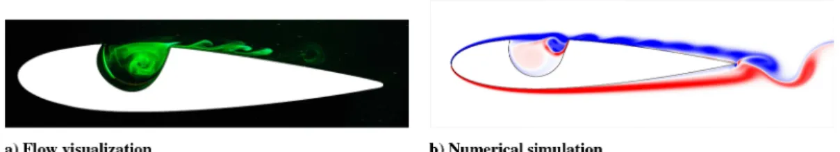
In Figs. 11 and 12, flow visualizations taken at two different instants in time, both at0andRe
c2104, are shown on the left and the corresponding vorticity plots of the numerical simulations are on the right. In all thefigures, the direction of theflow is from left to right.
The experiments clearly show shear-layer oscillations that are qualitatively similar to those observed in the simulations.§They also show mode switching between thefirst (Fig. 11) and second (Fig. 12) shear-layer modes at different instants in time. A similar mode switching has been observed for cavities on planar walls [17]. Estimates of the hydrodynamic wavelengthof the structures down-stream of the cavity reveal that=W1and=W0:5for thefirst and second modes, consistent with Rossiter’s [18] observations.
However, thefirst shear-layer mode appears to be more vigorous in the simulations, with much greater interaction between the shear layer and the vortical structures within the cavity. Without more detailed measurements, it is not possible to draw afirm conclusion, but our expectation is that, consistent with previous two-dimensional simulations of cavityflows [19], the current simulations exaggerate the coherence of the vorticalflow in the cavity, whereas theflow in the experiments is likely to be modulated by three-dimensional instabilities of the recirculatingflow [20] and by the boundary layers at the spanwise ends of the cavity.
Another difference between the simulations and experiments is observed in the wake of the airfoil, especially at higher angles of attack (not shown). In the experiments, the dye was quickly diffused a) wing camera U water upper endplate lower endplate free surface
bottom of water channel b)
Fig. 10 The airfoil with cavity and endplates is placed vertically inside the water channel: a) photo of the airfoil with endplates and b) a schematic drawing of the setup in the water channel.
§We are limited to making qualitative comparisons, because dye visualization is not equivalent to vorticityfield visualization. Unfortunately, the computational data were not saved atfine enough time intervals to permit detailed particle tracking computations to be made.
in the wake, presumably due to a transition to turbulentflow that cannot be captured in two-dimensional simulations.
V.
Conclusions
Two-dimensional DNS results of theflow around a clean airfoil and an airfoil with a cavity have been presented. The main goal of these simulations was to explore the possibleflow regimes and to gain more insight into theflow physics. The low Reynolds number simulations of the clean airfoil have been compared with data from the literature andflow visualization carried out in a water channel. In general, the agreement of these simulations with experimental data is reasonable.
The relatively high thickness of the airfoil without a cavity causes a laminar separation, which initially starts approximately half a chord length from the leading edge at0. Besides the regular vortex shedding due to the separated boundary layers, a very low-frequency oscillation is present at 0. This low-frequency oscillation appears to be caused by a unique combination of geometry and Reynolds number.
For the airfoil with a cavity, theflow in the cavity displays two regimes. For positive angles, theflow in the cavity is dominated by the second shear-layer mode. For negative angles, theflow in the cavity displays behavior that appears similar to a cavity wake mode. For0, theflow in the cavity switches back and forth between the second shear-layer mode and the wake mode. However, if one applies a small disturbance, the wake mode disappears and only the second shear-layer mode remains. Thefirst and second shear-layer modes were also observed in flow visualizations performed in a water channel.
In general, the oscillations of the shear layer above the cavity generate small vortices, which suppress separation of the boundary layer downstream of the cavity. For0, theflow on the lower side of the airfoil separates at about 50% of the chord length from the leading edge, while the presence of the cavity causes theflow to be attached on the upper side; this asymmetry generates a positive lift force.
For 4and
6, theflow over the airfoil with a cavity separates forward of the cavity. In this case, the shear layer does not impinge on the surface of the airfoil. The shear layer interacts weakly with the sharp rear edge of the cavity, causing a breakup of the shear layer into small-scale structures. In this case, the shear layer is dominating the separation bubble behavior.
At very high angles of attack, theflow over the airfoil with a cavity separates well before the forward edge of the cavity, and the cavity is in the separation bubble. The separated flow displays a strong interaction with the cavity. At10, this interaction causes the
flow to shed smaller-scale structures than the airfoil without a cavity
at the same angle of attack. Consequently, the wake is narrower, and the lift-to-drag ratio of the configuration with a cavity is higher compared with the case without a cavity.
The simulations have revealed interestingflow physics associated with the interaction of no less than three different types of instabilities. These are thefirst- and second-cavity shear-layer modes and separation bubble behavior, which is forced by a shear-layer oscillation. More elaborate experiments and three-dimensional LESs would be a logical next step to obtain more data and physical insight.
Acknowledgments
The first author would like to acknowledge the European Community for sponsoring this research project under project number AST4-CT-2005-012139. The authors wish to acknowledge G. J. F. van Heijst, A. Hirschberg, R. R. Trieling, and J. F. H. Willems for support, guidance, and constructive suggestions.
References
[1] Kruppa, E., “A Wind Tunnel Investigation of the Kasper Vortex Concept,” AIAA 13th Annual Meeting and Technical Display Incorporating the Forum on the Future of Air Transportation, AIAA Paper 1977-0310, 1977.
[2] Chernyshenko, S., Galletti, B., Iollo, A., and Zannetti, L.,“Trapped Vortices and a Favourable Pressure Gradient,” Journal of Fluid Mechanics, Vol. 482, 2003, pp. 235–255.
doi:10.1017/S0022112003004026
[3] Bunyakin, A., Chernyshenko, S., and Stepanov, G., “Inviscid Batchelor-Model Flow past an Aerofoil with a Vortex Trapped in a Cavity,”Journal of Fluid Mechanics, Vol. 323, 1996, pp. 367–376. doi:10.1017/S002211209600095X
[4] Bunyakin, A., Chernyshenko, S., and Stepanov, G.,“ High-Reynolds-Number Batchelor-Model Asymptotics of a Flow past an Aerofoil with a Vortex Trapped in a Cavity,”Journal of Fluid Mechanics, Vol. 358, 1998, pp. 283–297.
doi:10.1017/S0022112097008203
[5] Rowley, C., and Williams, D., “Dynamics and Control of High-Reynolds-Number Flow over Open Cavities,”Annual Review of Fluid Mechanics, Vol. 38, No. 1, 2006, pp. 251–276.
doi:10.1146/annurev.fluid.38.050304.092057
[6] Rockwell, D., and Naudasher, E.,“Review: Self-Sustained Oscillations of Flow Past Cavities,”Journal of Fluids Engineering, Vol. 100, No. 2, 1978, pp. 152–165.
doi:10.1115/1.3448624
[7] Gharib, M., and Roshko, A.,“The Effect of Flow Oscillations on Cavity Drag,”Journal of Fluid Mechanics, Vol. 177, 1987, pp. 501–530. doi:10.1017/S002211208700106X
[8] Taira, K., and Colonius, T.,“The Immersed Boundary Method: A Projection Approach,”Journal of Computational Physics, Vol. 225, No. 2, 2007, pp. 2118–2137.
doi:10.1016/j.jcp.2007.03.005
Fig. 11 Flow visualization of thefirst shear-layer mode in the water channel and the vorticity contour plot for the airfoil with a cavity at0and
Rec2104.
Fig. 12 Flow visualization of the second shear-layer mode in the water channel and the vorticity contour plot for the airfoil with a cavity at0and
[9] Colonius, T., and Taira, K.,“A Fast Immersed Boundary Method Using a Nullspace Approach and Multidomain Far-Field Boundary Conditions,”Computer Methods in Applied Mechanics and Engineer-ing, Vol. 197, Nos. 25–28, 2008, pp. 2131–2146.
doi:10.1016/j.cma.2007.08.014
[10] Nakano, T., Fujisawa, N., and Lee, S.,“Measurement of Tonal-Noise Characteristics and Periodic Flow Structure Around NACA0018 Airfoil,”Experiments in Fluids, Vol. 40, No. 3, 2006, pp. 482–490. doi:10.1007/s00348-005-0089-2
[11] Zaman, K., McKinzie, D., and Rumsey, C.,“A Natural Low-Frequency Oscillation of the Flow over an Airfoil Near Stall Conditions,”Journal of Fluid Mechanics, Vol. 202, 1989, pp. 403–442.
doi:10.1017/S0022112089001230
[12] Jacobs, E., and Sherman, A., “Airfoil Section Characteristics as Affected by Variations of the Reynolds Number,”NACA Rept. 586, 1937.
[13] Timmer, W.,“Two-Dimensional Low-Reynolds Number Wind Tunnel Results for Airfoil NACA 0018,”Wind Engineering, Vol. 32, No. 6, 2008, pp. 525–537.
doi:10.1260/030952408787548848
[14] Sarohia, V.,“Experimental and Analytical Investigation Of Oscillations in Flows over Cavities,”Ph.D. Thesis, California Inst. of Technology, Pasadena, CA, 1975.
[15] Michalke, A.,“On Spatially Growing Disturbances in an Inviscid Shear
Layer,”Journal of Fluid Mechanics, Vol. 23, No. 3, 1965, pp. 521–544. doi:10.1017/S0022112065001520
[16] Raju, R., Mittal, R., and Cattafesta, L.,“Dynamics of Airfoil Separation Control Using Zero-Net Mass-Flux Forcing,”AIAA Journal, Vol. 46, No. 12, 2008, pp. 3103–3115.
doi:10.2514/1.37147
[17] Kegerise, M., Spina, E., Garg, S., and Cattafesta, L.,“Mode-Switching and Nonlinear Effects in Compressible Flow Over a Cavity,”Physics of Fluids, Vol. 16, No. 3, 2004, pp. 678–687.
doi:10.1063/1.1643736
[18] Rossiter, J.,“Wind-Tunnel Experiments on the Flow over Rectangular Cavities at Subsonic and Transonic Speeds,”Aeronautical Research Council Reports and Memoranda 3438, 1964.
[19] Rowley, C., Colonius, T., and Basu, A.,“On Self-Sustained Oscillations in Two-Dimensional Compressible Flow over Rectangular Cavities,” Journal of Fluid Mechanics, Vol. 455, 2002, pp. 315–346.
doi:10.1017/S0022112001007534
[20] Bres, G., and Colonius, T.,“Three-Dimensional Instabilities in Com-pressible Flow over Open Cavities,” Journal of Fluid Mechanics, Vol. 599, 2008, pp. 309–339.
doi:10.1017/S0022112007009925
C. Bailly