Spectrum sensing algorithms and software-defined radio implementation for cognitive radio system

(1)

Repository ISTITUZIONALE

Spectrum sensing algorithms and software-defined radio implementation for cognitive radio system / Riviello, DANIEL GAETANO. - (2016).

Original

Publisher:

Published

DOI:10.6092/polito/porto/2641328 Terms of use:

Altro tipo di accesso

Publisher copyright

(Article begins on next page)

This article is made available under terms and conditions as specified in the corresponding bibliographic description in the repository

Availability:

This version is available at: 11583/2641328 since: 2016-05-03T11:42:50Z Politecnico di Torino

(2)

POLITECNICO DI TORINO

DOCTORAL SCHOOL

PhD program in Electronics and Communications

Engineering – XXVIII Cycle

Doctoral dissertation

Spectrum sensing algorithms and

software-defined radio

implementation for cognitive radio

systems

Daniel Gaetano

_Riviello

Supervisor Coordinator of the PhD program

(3)

(4)

Summary

The scarcity of spectral resources in wireless communications, due to a fixed frequency allocation policy, is a strong limitation to the increasing demand for higher data rates. However, measurements showed that a large part of frequency channels are underutilized or almost unoccupied.

Thecognitive radio paradigm arises as a tempting solution to the spectral conges-tion problem. A cognitive radio must be able to identify transmission opportunities in unused channels and to avoid generating harmful interference with the licensed primary users. Its key enabling technology is the spectrum sensing unit, whose ultimate goal consists in providing an indication whether a primary transmission is taking place in the observed channel. Such indication is determined as the result of a binary hypothesis testing experiment wherein null hypothesis (alternate hypothesis) corresponds to the absence (presence) of the primary signal.

The first parts of this thesis describes the spectrum sensing problem and presents some of the best performing detection techniques. Energy Detection and multi-antenna Eigenvalue-Based Detection algorithms are considered. Important aspects are taken into account, like the impact of noise estimation or the effect of primary user traffic. The performance of each detector is assessed in terms of false alarm probability and detection probability.

In most experimental research, cognitive radio techniques are deployed in software-defined radio systems, radio transceivers that allow operating parameters (like

modu-lation type, bandwidth, output power, etc.) to be set or altered by software.

In the second part of the thesis, we introduce the software-defined radio concept. Then, we focus on the implementation of Energy Detection and Eigenvalue-Based Detection algorithms: first, the used software platform, GNU Radio, is described, secondly, the implementation of a parallel energy detector and a multi-antenna eigenbased detector is illustrated and details on the used methodologies are given. Finally, we present the deployed experimental cognitive testbeds and the used radio peripherals.

The obtained algorithmic results along with the software-defined radio implemen-tation may offer a set of tools able to create a realistic cognitive radio system with real-time spectrum sensing capabilities.

(5)

This thesis is the result of a 3-year research activity during which I have met and collaborated with amazing people.

I would like to express my deepest gratitude to my Ph.D. advisor, Prof. Roberto Garello, who was my Master’s thesis advisor too, and guided and supported me in all possible ways ever since.

I would like to thank Dr. Alberto Perotti and Andrea Molino for hosting me at CSP - ICT Innovation for more than one year. I had the chance to work with great colleagues like Eng. Floriana Crespi and Simone Scarafia. The project described in Chap.9was done during that period and I especially want to thank Eng. Ferdinando Ricchiuti for his assistance.

Likewise, I am grateful to Eng. Claudio Pastrone and Dr. Hussein Khaleel for hosting me at the Pervasive Technologies Research Lab of Istituto Superiore Mario Boella (ISMB).

I am also grateful to Prof. Jean-Marie Gorce, who gave me the great opportunity to spend my last year at the Centre of Innovation in Telecommunications and Integration of service (CITI) Laboratory in Lyon. I had the chance to work with advanced radio equipment, as described in Chap. 11. A special thanks goes to Dr. Yasser Fadlallah for his support during my stay at CITI Lab.

Finally, I want to sincerely thank my friend and colleague Pawan Dhakal for our fruitful and lasting collaboration, Dr. Giuseppa Alfano for her help in the reviewing process, and, last but not least, my family and everyone who supported me during these years.

(6)

Publications

Some of the contents of this thesis have previously appeared or are going to appear in the following publications:

Book chapters

• Daniel Riviello, Sergio Benco, Floriana Loredana Crespi, Andrea Ghittino, Roberto Garello and Alberto Perotti, “Spectrum Sensing Algorithms for Cogni-tive TV White-Spaces System”, in Cognitive Communication and Cooperative HetNet Coexistence, Springer International Publishing, pp. 71-90, 2014. ISBN: 978-3-319-01402-9. DOI: 10.1007/978-3-319-01402-9_4.

• A. F. Cattoni, O. Tonelli, J. L. Buthler, L. da Silva, C.L. Miranda, P. Sutton, F. Crespi, S. Benco, A. Perotti and D. Riviello, “Designing a CR Test Bed: Practical Issues”, inCognitive Radio and Networking for Heterogeneous Wireless Networks, Springer International Publishing, pp. 315-360, 2015. ISBN: 978-3-319-01718-1, DOI: 10.1007/978-3-319-01718-1_12.

Journal papers

• Daniel Riviello, Sergio Benco, Floriana Crespi, Alberto Perotti and Roberto Garello, “Spectrum Sensing in the TV White Spaces”, International Journal on Advances in Telecommunications, vol. 6, n. 3-4, pp. 109-122, Dec. 2013. ISSN: 1942-2601.http://www.thinkmind.org/download.php?articleid=tele_v6_ n34_2013_4

(7)

• Daniel Riviello, Sergio Benco, Floriana Crespi, Alberto Perotti and Roberto Garello, “A comparison between multi-sensor and CP-based spectrum sensing for TV white spaces”, Proceedings of the 3rd International workshop of COST Action IC0902, Ohrid (MK), September 12-14, 2012.

• Daniel Riviello, Sergio Benco, Floriana Crespi, Alberto Perotti and Roberto Garello, “Sensing of DVB-T Signals for White Space Cognitive Radio System”,

COCORA 2013, The Third International Conference on Advances in Cognitive Radio, Apr. 2013, pp. 12-17. ISBN: 978-1-61208-267-7.http://www.thinkmind. orgindex.phpview=article&articleid=cocora_2013_1_30_60031

? Best Paper Award: http://www.iaria.org/conferences2013/ awardsCOCORA13/cocora2013_a1.pdf

• Pawan Dhakal, Roberto Garello, Federico Penna and Daniel Riviello, “Impact of noise estimation on eigenvalue based spectrum sensing in cognitive radio sys-tems”, Proceedings of the 4th International workshop of COST Action IC0902, Rome, October 9-11, 2013. http://newyork.ing.uniroma1.it/IC0902/4th-Workshop/Technical_contributions/October_9/Session_1/06_IC0902_ 4th_Workshop_contribution_Riviello.pdf

• Daniel Riviello, Pawan Dhakal, Roberto Garello and Federico Penna, “Hybrid Approach Analysis of Energy Detection and Eigenvalue Based Spectrum Sensing Algorithms with Noise Power Estimation”,COCORA 2014, The Fourth Inter-national Conference on Advances in Cognitive Radio, Nice, 23-27 Feb. 2014, pp. 20-25. http://www.thinkmind.org/download.php?articleid=cocora_ 2014_1_40_80029

• Pawan Dhakal, Roberto Garello, Federico Penna and Daniel Riviello, “Impact of Noise Estimation on Energy Detection and Eigenvalue Based Spectrum Sensing Algorithms”,Communications (ICC), 2014 IEEE International Conference on, Sydney, 10-14 Jun. 2014, pp. 1367-1372, DOI: 10.1109/ICC.2014.6883512. • P. Dhakal, D. Riviello, R. Garello, “SNR Wall Analysis of Multi-Sensor Energy

Detection with Noise Variance Estimation”, Wireless Communications Systems (ISWCS), 2014 11th International Symposium on, Barcelona, 26-29 Aug. 2014,

pp. 680-684. DOI: 10.1109/ISWCS.2014.6933440.

• Daniel Riviello, Pawan Dhakal, Roberto Garello, “On the Use of Eigenvectors in Multi-Antenna Spectrum Sensing with Noise Variance Estimation”, Signal Processing and Integrated Networks (SPIN), 2015 2nd International Conference on, Noida, 19-20 Feb. 2015, pp. 44-49, DOI: 10.1109/SPIN.2015.7095339.

(8)

• Daniel Riviello, Pawan Dhakal, Roberto Garello, “Performance Analysis of Multi-Antenna Hybrid Detectors and Optimization with Noise Variance Esti-mation”, COCORA 2015, The Fifth International Conference on Advances in Cognitive Radio, Barcelona, 19-24 Apr. 2015, pp. 14-19, ISBN: 978-1-61208-403-9. http://www.thinkmind.org/download.php?articleid=cocora_2015_1_ 30_80029

• Pawan Dhakal, Daniel Riviello, “Multi-Antenna Energy Detector Under Un-known Primary User Traffic”, COCORA 2016, The Sixth International Confer-ence on Advances in Cognitive Radio, Lisbon, 21-25 Feb. 2016, pp. 15-20, ISBN: 978-1-61208-456-5. http://www.thinkmind.org/download.php?articleid= cocora_2016_1_40_80032

? Best Paper Award: http://www.iaria.org/conferences2016/ awardsCOCORA16/cocora2016_a1.pdf

• Pawan Dhakal, Shree K. Sharma, Symeon Chatzinotas, Björn Ottersten, and Daniel Riviello, “Effect of Primary User Traffic on Largest Eigenvalue Based Spectrum Sensing Technique”, Cognitive Radio Oriented Wireless Networks (CROWNCOM), 2016 11th EAI International Conference on, Grenoble, May

(9)

Summary _iii

Acknowledgements _iv

Publications _v

List of Acronyms _xvii

1 Introduction ₁

1.1 Spectrum sensing algorithms . . . 5

1.2 Software defined-radio implementation . . . 5

1.3 Thesis organization . . . 6

I

Spectrum sensing theory

9

2 System model and test statistics ₁₁ 2.1 State of the art . . . 12

2.2 Problem formulation . . . 14

2.2.1 Mathematical framework . . . 15

2.2.2 The Neyman-Pearson test . . . 17

2.3 Test statistics . . . 18

2.3.1 Energy Detection . . . 18

2.3.2 Eigevalue-Based Detection algorithms . . . 21

2.3.3 Roy’s Largest Root Test (RLRT) . . . 25

2.3.4 Generalized Likelihood Ratio Test (GLRT) . . . 27

3 Sensing techniques for cognitive TV White-Spaces systems ₂₉ 3.1 Primary signal. . . 30

3.2 Single antenna spectrum sensing algorithms . . . 34

3.2.1 Cyclic prefix based detector . . . 34

(10)

3.3 Multi-antenna spectrum sensing algorithms. . . 38

3.3.1 System model . . . 39

3.3.2 Known noise variance algorithms . . . 40

3.3.3 Unknown noise variance algorithms . . . 40

3.4 Channel models . . . 40

3.4.1 Additive White Gaussian Noise (AWGN) channel . . . 41

3.4.2 Flat Rayleigh fading channel . . . 41

3.4.3 Typical Urban 6-path (TU6) channel . . . 41

3.5 Performance assessment and trade-offs . . . 43

3.5.1 Results . . . 43

4 Hybrid Energy and Eigenvalue-based Detection algorithms with noise variance estimation ₅₃ 4.1 Noise estimation . . . 53

4.1.1 Offline noise estimation: hybrid approach 1 . . . 53

4.1.2 Online noise estimation: hybrid approach 2 . . . 55

4.2 Hybrid Energy Detection . . . 55

4.2.1 Hybrid ED approach 1 (HED1) . . . 55

4.2.2 Hybrid ED approach 2 (HED2) . . . 57

4.3 Hybrid Roy’s Largest Root Test . . . 59

4.3.1 Hybrid RLRT approach 1 (HRLRT1) . . . 59

4.3.2 Hybrid RLRT approach 2 (HRLRT2) . . . 61

4.4 Results . . . 63

4.5 Optimization of Hybrid Energy Detection. . . 67

5 EigenVEctor (EVE) Test and hybrid variant ₇₁ 5.1 EigenVEctor (EVE) Test . . . 71

5.2 Hybrid and blind variant of EVE . . . 72

5.2.1 Neyman-Pearson Test . . . 72

5.3 Simulation results . . . 73

6 SNR Wall for multi-antenna Energy Detection ₈₁ 6.1 Multi-antenna ED and SNR Wall . . . 81

6.2 Noise uncertainty distribution and formulation of uncertainty bound . 85 6.3 Simulation results . . . 88

7 Effect of primary user traffic on Energy and Eigenvalue-based De-tection algorithms ₉₁ 7.1 System model . . . 92

7.2 Characterization of Primary User traffic . . . 93

(11)

7.5 RLRT performance analysis . . . 103

7.6 Numerical results for RLRT . . . 108

II

GNU Radio Software defined-radio (SDR)

implementa-tion

113

8 SDR testbeds and GNU Radio ₁₁₅ 8.1 SDR concept . . . 115

8.2 SDR and testbeds . . . 117

8.2.1 SDR peripherals . . . 118

8.3 GNU Radio . . . 119

8.3.1 How to create a custom block . . . 120

9 Parallel Energy Detector implementation 127 9.1 Digital Mobile Radio (DMR). . . 127

9.2 USRP1 . . . 128

9.3 GNU Radio flowgraph . . . 129

9.4 Energy detection . . . 133

9.5 Noise estimation and update . . . 139

9.6 External Graphical User Interface (GUI) . . . 144

10 Eigenvalue-based detector implementation ₁₄₇ 10.1 Description of the eigenbased block . . . 147

10.2 Threshold computation . . . 148 10.2.1 RLRT . . . 148 10.2.2 GLRT . . . 150 10.3 Eigenvalue algorithm . . . 151 10.3.1 Lanczos algorithm . . . 151 10.3.2 Bisection algorithm . . . 152

10.4 Eigenbased block code . . . 155

10.5 Simulation results . . . 164

11 Software-defined radio peripherals for multi-antenna cognitive testbeds₁₆₇ 11.1 NI USRP-2920 . . . 167

11.1.1 GNU Radio eigenvalue-based testbed . . . 168

11.1.2 Results and issues . . . 170

11.2 Nutaq PicoSDR 4x4 . . . 171

11.2.1 PicoSDR and GNU Radio . . . 172

(12)

12 Conclusion and future work ₁₇₉

(13)

2.1 Receiver Parameter for 802.22 WRAN [18]. . . 12

3.1 Main parameters of DVB-T. . . 30

3.2 Typical Urban profile (TU6). . . 42

(14)

List of Figures

1.1 OFCOM frequency allocation chart for UK [1].. . . 2

1.2 Spectrum occupancy chart [4]. . . 3

3.1 Encoder block. . . 31

3.2 Modulator block. . . 31

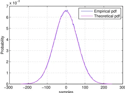
3.3 Estimated vs. theoretical pdf of the DVB-T signal, real part. . . 32

3.4 Estimated vs. theoretical pdf of the DVB-T signal, imaginary part. . 32

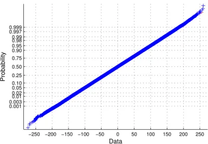
3.5 Quantile-quantile plot of the DVB-T signal, real part. . . 33

3.6 Quantile-quantile plot of the DVB-T signal, imaginary part. . . 33

3.7 OFDM symbol structure with cyclic prefix. . . 34

3.8 Symbol autocorrelation after CP insertion - Amplitude - 8k mode. . . 35

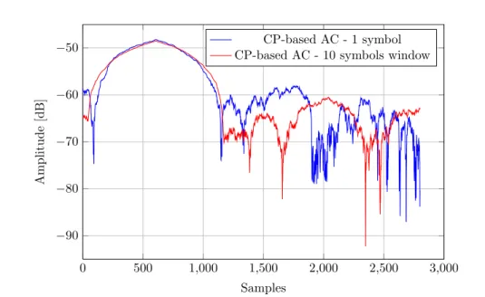
3.9 Amplitude of the CP-based auto-correlation, 1 symbol vs. 10 symbols observation. . . 37

3.10 Cross-correlation between DVB-T signal and only-pilot signal. . . 38

3.11 Eigenvalue-based detectors, DVB-T 8k PU signal, flat fading channel, N = 50, K = 10, ROC curves (SNR = -10dB).. . . 45

3.12 Eigenvalue-based detectors, DVB-T 8k PU signal, flat fading channel, N = 50, K = 10, Pd vs. SNR (Pf a = 0.01). . . 45

3.13 Eigenvalue-based detectors, DVB-T 8k PU signal, flat fading channel, N = 200, K = 4, ROC curves (SNR = -10dB).. . . 47

3.14 Eigenvalue-based detectors, DVB-T 8k PU signal, flat fading channel, N = 200, K = 4, Pd vs. SNR (Pf a = 0.01). . . 47

3.15 GLRT detection probability as a function of time (samples) and sensors through flat-fading channel, SNR = -10dB, Pf a = 0.01. . . 48

3.16 GLRT detection probability as a function of time (samples) and sensors through flat-fading channel, SNR = -15dB, Pf a = 0.01. . . 49

3.17 Eigenvalue-based detectors, DVB-T 8k PU signal, TU6 channel model, N = 50, K = 10, ROC curves (SNR = -10dB).. . . 49

3.18 Eigenvalue-based detectors, DVB-T 8k PU signal, TU6 channel model, N = 50, K = 10, Pd vs. SNR (Pf a = 0.01). . . 50

(15)

PU signal, flat fading channel, N = 50, K = 10, ROC curves (SNR =

-10dB). . . 50

3.20 CP-based vs. eigenvalue-based (unknownσ_v2) detectors, DVB-T 8k PU signal, flat fading channel, N = 200,K = 4, Pd vs. SNR (Pf a= 0.01). 51 4.1 HED1/HRLRT1 with offline noise estimation approach. . . 54

4.2 HED2/HRLRT2 with online noise estimation approach. . . 56

4.3 Theoretical and numerical ROC plot of HED1/HRLRT1, N = 80, M = 80, K = 4, SNR = ₋10dB. . . 64

4.4 Theoretical and numerical ROC plot of HED2/HRLRT2, N = 80, M = 80, K = 4, SNR = ₋10dB. . . 64

4.5 Performance curves of ED and its hybrid approaches,N = 10,M = 10, K = 5, Pf a = 0.05. . . 65

4.6 Performance curves of RLRT and its hybrid approaches, N = 80, M = 80, K = 4,Pf a = 0.05. . . 65

4.7 ROC curves of ED/RLRT and their hybrid approach 1 (HED1/HRLRT1), N = 80, M = 80, K = 4, SNR = ₋10 dB. . . 66

4.8 Effect of noise variance fluctuation on ED and RLRT,N = 100,K = 4, Var(ˆσ2_v) = 0.0032 (₋25 dB) given nominal noise varianceσ_v2 = 1. . . . 66

4.9 Probability of detection as a function of M given M +N =const. . . 69

5.1 Performance curve, P dvs. SNR, K = 4, N = 200. . . 74 5.2 ROC curve, K = 4, N = 200. . . 75 5.3 Performance curve, P dvs. SNR, K = 8, N = 200. . . 76 5.4 ROC curve, K = 8, N = 200. . . 76 5.5 Performance curve, P dvs. SNR, K = 4, N = 100. . . 77 5.6 ROC curve, K = 4, N = 100. . . 77

5.7 Performance curve, P dvs. SNR, with 2, 4, 6 auxiliary slots. . . 78

5.8 ROC curve, with 2, 4, 6 auxiliary slots. . . 78

5.9 Performance curve, P dvs. K,N = 100.. . . 79

5.10 Performance curve, P dvs. N, K = 4. . . 79

6.1 Comparison of sample complexity N for a given Pd and Pf a in a single and multi-antenna scenario as a function of the SNR, Pd = 0.9, Pf a= 0.1. . . 82

6.2 Variation of the sample complexity N as the SNR approaches the SNR Wall for ED, K = 5, P_d0 = 0.9, P_{f a}0 = 0.1[x= 10 log₁₀β in (6.14)]. 85 6.3 Probability distribution of the normalized noise variance estimate V, S = 2,K = 2, M = 10. . . 86

6.4 Variation of the noise uncertainty level as a function of the slots S used for noise variance estimation, K = 4, M = 100.. . . 87

6.5 Variation of the SNR Wall level as a function of auxiliary slots S used for noise variance estimation, K = 4, M = 100. . . 88

(16)

6.6 Variation of the sample complexity N as the SNR approaches the

SNR Wall with different values of auxiliary slots S, K = 4, M = 100,

α = 0.0001. . . 89

7.1 Primary user traffic scenario and sensing slot classification. . . 94

7.2 ED probability density functions, N = 50, K = 4, Mf = 150, Mb = 150,SNR = ₋6dB. . . 101

7.3 ROC curve performance, N = 100, K = 4, SNR = ₋6 dB. . . 102

7.4 Probability of misdetection vs. number of antennas K, N = 25, Mf = 62,Mb = 62,Pf a = 0.1. . . 103

7.5 Probability of misdetection vs. SNR, N = 25, K = 4,Pf a = 0.1. . . . 104

7.6 ROC curve performance, N = 50, K = 4, SNR = -6 dB. . . 109

7.7 Probability of misdetection vs. SNR, K = 8, Pf a = 0.01,Mf =Mb = 3000. . . 110

7.8 Misdetection probability vs. number of antennas K, N = 100, Pf a = 0.01, Mf =Mb = 1500. . . 111

7.9 Detection probability vs. number of samplesN, SNR= -10 dB,K = 8, Pf a= 0.01. . . 112

8.1 Ideal SDR concept. . . 116

8.2 Typical SDR scheme. . . 117

8.3 Example of a block with two inputs and two outputs. . . 124

8.4 Example of connected blocks in GRC.. . . 125

9.1 USRP1 with Basic RX daughterboard used for the testbed. . . 128

9.2 USRP1 schematic. . . 129

9.3 Parallel Energy Detector diagram. . . 130

9.4 GNU Radio flowgraph for parallel Energy Detector. . . 131

9.5 Parallel Energy Detector block with parameters. . . 133

9.6 Flowgraph for initial noise estimation. . . 139

9.7 Function probe block.. . . 143

9.8 External GUI architecture. . . 144

9.9 Signal spectrum and waterfall. . . 145

10.1 Eigenbased block with parameters. . . 148

10.2 Simulation flowgraph for the eigenbased block. . . 164

10.3 WX GUI of the simulation flowgraph foreigenbased block. . . 166

10.4 Performance curve (Pd vs. SNR) for the eigenbased block. . . 166

11.1 USRP N210 schematic. . . 168

11.2 Multi-antenna eigenvalue-based detection testbed. . . 169

11.3 Flowgraph at the TX host with 1 USRP sink. . . 170

11.4 Flowgraph at the RX host with 4 USRP sources. . . 171

11.5 Nutaq PicoSDR 4x4 schematic. . . 173

11.6 Nutaq PicoSDR 4x4 with 4 Aaronia OmniLOG 70600 antennas. . . . 173

(17)

11.9 Flowgraph with PicoSDR 4x4 for EBD testbed. . . 177

11.10PicoSDR 4x4 spectrum and GLRT Pf a with no PU signal. . . 177

11.11PicoSDR 4x4 spectrum and GLRT Pf a with no PU signal and DC

(18)

List of Acronyms

AC Autocorrelation A/D Analog-to-Digital

AWGN Additive White Gaussian Noise BEVE Blind EigenVEctor Test

CDF Cumulative Distribution Function CP Cyclic Prefix

CR Cognitive Radio

CRN Cognitive Radio Network D/A Digital-to-Analog

DC Direct Current DMR Digital Mobile Radio

DSP Digital Signal Processor

DVB-T Digital Video Broadcasting - Terrestrial EBD Eigenvalue Based Detection

ED Energy Detection

ERD Eigenvalue Ratio Detector

EVE EigenVEctor Test

FFT Fast Fourier Transform

(19)

GRC GNU Radio Companion GUI Graphical User Interface IFFT Inverse Fast Fourier Transform

HED see HED1

HED1 Hybrid ED approach 1 with offline noise estimation HED2 Hybrid ED approach 2 with online noise estimation

HEVE Hybid EigenVEctor Test

HRLRT see HRLRT1

HRLRT1 Hybrid RLRT approach 1 with offline noise estimation HRLRT2 Hybrid RLRT approach 2 with online noise estimation

IEEE Institute of Electrical and Electronics Engineers I/Q In-phase and Quadrature

LRT Likelihood Ratio Test

LRT- Noise Independent Likelihood Ratio Test LTE Long Term Evolution

MAC Medium Access Control

MIMO Multiple-Input Multiple-Output

ML Maximum-Likelihood

NP Neyman-Pearson

OFDM Orthogonal Frequency-Division Multiplexing

pdf Probability Density Function pmf Probability Mass Function

PSK Phase-Shift Keying PU Primary User

(20)

QAM Quadrature Amplitude Modulation QPSK Quadrature Phase-Shift Keying

RF Radio Frequency

RLRT Roy’s Largest Root Test

RMT Random Matrix Theory

ROC Receiver Operating Characteristic SDR Software-defined Radio

SNR Signal-to-Noise Ratio SS Steady State

STA Station

SU Secondary User

TCP Transmission Control Protocol TS Transient State

TVWS TV White Spaces

TW2 Tracy-Widom distribution of order 2 UDP User Datagram Protocol

UMP Uniformly Most Powerful

USRP Universal Software Radio Peripheral

WiMAX Worldwide Interoperability for Microwave Access

WRAN Wireless Regional Area Network

(21)

(22)

Chapter 1 Introduction

The increasing demand for higher data rates in wired, and most of all, wireless technology is a consequence of the transition from voice-only communications to multimedia type applications. Wireless communication has been the fastest growing segment of the communications industry in the past few decades. Number of high speed data services (e.g., Zigbee, WiMax-Advanced, LTE, Ultra-wide Band Network), various applications (e.g., IP Television, high-speed wireless internet, cellular tele-phony including multimedia services) and supporting electronic devices (for example mobiles, tablets, computers) are just some of the advances in the field of wireless communications that can be named. Moreover, many new research works on Wireless Sensor Network (WSN), Next Generation Networking (NGN) services, telemedicine, smart home appliances and many more certainly demand for the new band allocations of radio spectrum.

Wireless channels are characterized by a fixed spectrum assignment policy. Elec-tromagnetic spectrum is strictly regulated and licenced by governmental entities, for instance, the Federal Communication Commission (FCC) in United States, the Office of Communications (OFCOM) in UK and Ministero dello Sviluppo Economico - Dipartimento per le Comunicazioni in Italy. The rapid development in the field of wireless communications certainly creates a big challenge for every licensing organi-zation to accommodate all the new applications and services noted above with the limited electromagnetic spectrum. The frequency allocation chart of UK [1] in Fig.1.1

shows that large portion of the radio spectrum is already assigned to traditional services (Mobile, Maritime Mobile, Fixed Satellite Services, Radio Navigation), and the same applies to Italy [2] and US. Although some unlicensed bands are available, such as the industrial, scientific and medical (ISM) band in2.4GHz, which could be

the possible solution for accommodating new services, multiple wireless technologies are already deployed in these bands such as 802.11 Wireless Local Area Network

(WLAN), cordless phones, Bluetooth, Wireless Personal Area Network (WPAN), etc. Some other examples of unlicenced frequency bands include U-NII Unlicensed

(23)

Part of the Chemring Group

Figure 1.1: OFCOM frequency allocation chart for UK [1].

National Information Infrastructure U-NII-1 and U-NII-2 bands where systems such as IEEE802.11a WLAN and IEEE802.11n WLAN operate.

However, the measurements carried out indicate a distinct difference in the frequency channel usage where a larger part of frequency channels are partially occupied or almost unoccupied [3] (see Fig.1.2). Some of these unoccupied frequency bands are allocated to broadcasting services and referred to as white spaces. In some cases, these hardly used bands are specifically assigned for a purpose, such as guard band to prevent interference while in other cases these white spaces exist naturally between used channels. That is because assigning nearby transmissions to immediate adjacent channels will create destructive interference to both channels. In addition to white space assigned for technical reasons, there is also unused radio spectrum which has either, never been used or is becoming free as a result of technical changes.

For all these reasons, the need for adopting new techniques with capability of exploiting the available spectrum arises.Cognitive radio (CR) is standing out to be a tempting solution to the spectral congestion problem since it introduces a proper exploitation in the utilization of the frequency bands that are not largely occupied by licensed users [5]. Below is the formal definition of Cognitive Radio adopted by

(24)

Figure 1.2: Spectrum occupancy chart [4]. the Federal Communication Commission (FCC) [6]:

A radio or system that senses its operational electromagnetic enviroment and can dynamically and autonomously adjust its radio operating param-eters to modify system operation, such as maximize throughput, mitigate interference, facilitate interoperability, access secondary markets.

Here’s another definition given by IEEE-USA [7]:

A radio frequency transmitter/receiver that is designed to intelligently detect whether a particular segment of the radio spectrum is currently in use, and to jump into (and out of, as necessary) the temporarily-unused spectrum very rapidly, without interfering with the transmissions of other authorized users.

The key feature of a CR is the capability to locally exploit in an autonomous way the unused spectrum providing new ways for spectrum access. Spectrum sensing

(25)

remains a key enabling technology for cognitive radios. They have to sense, measure, learn, and have a full awareness of the parameters related to the radio channel char-acteristics in order to identify spectrum opportunities and maybe most importantly, prevent interference with the licensed primary users (PUs).

The termprimary users refers to the users with higher priority or legacy rights on the use of a specific part of the spectrum andsecondary users refers to the users with lower priority. The secondary ones exploit the spectrum in a way that prevents them from causing interference to the primary users. This poses the need for secondary users to have cognitive radio capabilities that include sensing the spectrum reliably. By sensing reliably, it simply means that the secondary users should be in a position to check whether the spectrum is being used by the primary user. Additionally, cognitive radios should be able to change the parameters of the radio transceiver in order to exploit the unused part of it [8].

The concept of spectrum sensing is similar in some ways to the multiple access method used in IEEE 802.11, Carrier sense multiple access with collision avoidance

(CSMA/CA), in which a station (STA) senses the channel in order to gain access and to send data in a basic service set (BSS). The biggest difference is that a station in IEEE 802.11 senses only a well-defined channel, 20 MHz in the ISM radio bands around 2.4 GHz, while a cognitive radio system must be able to sense and scan the whole spectrum or at least a larger portion of it.

The crucial task in spectrum sensing lies in the decision making as to whether a primary signal is present or not. Detection theory is a field of statistical signal processing where optimal or highly reliable decision making procedures are developed. The data sets obtained from the observations are assumed to be samples of continuous-time waveforms or a sequences of data points. This decision making process is formulated as a hypothesis testing problem. In common cases, the null hypothesis offers a description of the scenario in which only noise is present and when the PU is not active. The alternate hypothesis describes the scenario where primary transmission is present in the noisy observations [9].

During decision making, errors may occur and there are two types of error likely to take place; the first one is known as false alarm and the second one is misdetection. Looking at the first one, the error occurs when one decides that the primary is active based on the information (data) that comes from distribution corresponding to null hypothesis. This false alarm leads us to an unnecessary reduction of the secondary use of spectrum. Therefore, it is highly crucial to control the false alarm rate. The latter occurs when there is a failure of detecting PU activity leading us to a conclusion of availability of spectrum for secondary use and this type of error creates interference with PU signals, consequently retransmissions and reduced rate for both primary and secondary systems. Moreover, harmful interference is caused to licensed systems that have paid for the spectrum [9].

(26)

1.1 – Spectrum sensing algorithms

1.1 Spectrum sensing algorithms

Several spectrum sensing methods have been proposed for Cognitive Radio applica-tions including Energy Detection (ED) [10], Matched Filtering [11], Feature Detection Algorithms [12]. Energy Detection does not make any assumption on the PU signal statistics while the matched filter detection algorithms assume the complete knowl-edge on the pilot waveform or the preamble to design the detectors. Feature detection lies in the middle of these two extremes and only makes certain assumptions on the statistical properties of the PU signal. Even though Matched Filtering and feature detection algorithms are known to outperform Energy Detection, the requirement of the knowledge of the PU signal characteristics and the long sensing period makes them less suitable for spectrum sensing in Cognitive Radio Networks (CRN), since the knowledge of the PU signal is usually unavailable. Thus, for Cognitive Radio applications, ED is considered to be the simplest and most popular sensing algorithm which compares the energy of the received signal to the noise variance. In recent years, sensing techniques based on the eigenvalues of the received covariance matrix evolved as a promising solution for spectrum sensing. Eigenvalue-Based detection (EBD) schemes are further categorized as “semi-blind EBD”, in which the noise level is assumed to be known, and “blind EBD”, in which the noise level is not known. Methods belonging to the first class provide better performance especially when the noise variance is exactly known, whereas blind methods are more robust to uncertain or varying noise level.

1.2 Software defined-radio implementation

The software-defined radio (SDR) concept has been introduced almost twenty years ago in [13] and it is innovative even nowadays. The main scope of SDR is to improve the flexibility of radio communication devices by implementing the digital sections entirely in software using dedicated or general-purpose processors. A software-defined radio system is a radio communication system where components that have been typically implemented in hardware (e.g., mixers, filters, amplifiers, modulators/de-modulators, etc.) are instead implemented by means of software on a personal computer or embedded computing devices.

Different SDR platforms have been developed in recent and past years. Among these, an open platform called GNU Radio [14] has prevailed firstly in the academic community and it is becoming frequently adopted even in industrial projects. GNU Radio is a free and open-source software development toolkit that provides signal processing blocks to implement software-defined radios and signal processing systems. GNU Radio is not primarily a simulation tool, although it can be used for this purpose. The GNU Radio infrastructure is written entirely in C++, it is composed

(27)

of a wide collection of signal processing blocks. A set of interconnected blocks forms a flowgraph, which can be written both in C++ or in Python. GNU Radio provides also a Graphical User Interface (GUI), called GNU Radio Companion (GRC). It is possible to create new blocks in addition to the existing ones.

When paired with suitable RF front-ends, a real radio communication system can be carried out. The combination of a computer with GNU Radio installed and an RF front-end allows the creation of affordable SDR testbeds. A lot of hardware vendors provide GNU Radio support for their products, ranging from very expensive measurement-quality systems, to very cheap receiver hardware, but the most commonly used with GNU Radio are the Universal Software Radio Peripheral (USRP) devices by Ettus Research and National Instruments.

The implementation of spectrum sensing algorithms in a SDR platform is a crucial task for the construction of a cognitive system prototype. Sensing techniques have been implemented in GNU Radio for instance in [15, 16]. In this work, Energy Detection and Eigenvalue-Based Detection algorithms have been implemented in GNU Radio, more in detail a parallel Energy Detector designed for Digital Mobile Radio (DMR) signals and among the EBD algorithms the Roy’s Largest Root Test (RLRT) and the Generalized Likelihood Ratio Test (GLRT).

1.3 Thesis organization

This thesis focuses on several aspects of spectrums sensing algorithms. Part I illus-trates and assesses the performance of Energy Detection (ED) and Eigenvalue-Based Detection (EBD) test statistics, while PartII focuses on the software-defined radio (SDR) implementation in GNU Radio of the sensing algorithms. More in detail:

• Chap. 2introduces the sensing problem and the mathematical system model that will be used throughout the thesis. Moreover, analytical results are provided for Energy Detection (ED) and two of the main EBD algorithms: Roy’s Largest Root Test (RLRT) and the Generalized Likelihood Ratio Test (GLRT). • Chap. 3 focuses on the sensing of DVB-T signals. After a description of the

PU signal, a comparison between single-antenna parametric (feature-based) detectors and multi-antenna non parametric detectors is carried out. Simulations have been performed with different channel models.

• Chap. 4introduces the idea of auxiliary noise variance estimation and presents hybrid approaches for ED and RLRT. Analytical formulations for the new tests are provided and performance analysis for both approaches is carried out in order to asses the impact of the noise power estimation.

(28)

1.3 – Thesis organization

• Chap. 5presents the EigenVEctor Test (EVE), which exploits the eigenvector associated to the largest eigenvalue of the sample covariance matrix to estimate the channel. Results show EVE is able to outperform ED and EBD algorithms. • Chap. 6 presents the concept of SNR Wall phenomenon for ED and extends it to the multi-antenna ED case. The analytical expression of the uncertainty bound for multi-antenna ED is derived and proved to be independent of the number of antennas.

• Chap.7 studies the effect of primary user (PU) traffic on the performance of RLRT. A realistic and simple PU traffic model is considered, which is based only on the discrete time distribution of PU free and busy periods. Analytical expressions for the probability density functions of the decision statistic are derived and validated by simulations.

• Chap. 8 introduces the SDR and SDR-based testbed concepts, and presents the GNU Radio software platform. Since the implementation of ED and EBD algorithms required the creation of custom application in addition to the existing collection, the main focus of the chapter is on how to write a custom signal processing block in GNU Radio.

• Chap. 9 presents the first SDR implementation, a parallel Energy Detector designed to sense and collect occupancy statistics on Digital Mobile Radio (DMR) channels. The project was carried out in collaboration with CSP - ICT

Innovation.

• Chap.10presents the GNU Radio implementation of a multi-antenna eigenvalue-based detector, whose test statistic can be selected between RLRT and GLRT. The main focus of the chapter is the description of the eigenvalue algorithm (Lanczos method plus bisection).

• Finally, Chap. 11 presents the SDR peripherals, namely the National Instru-ments NI USRP 2920 and the Nutaq PicoSDR 4x4, and the multi-antenna cognitive testbeds deployed in the CITI Laboratory of INSA Lyon.

(29)

(30)

Part I

(31)

(32)

Chapter 2 System model and test statistics

Among the functionalities provided by Cognitive Radio, Opportunistic Spectrum Access (OSA) is devised as a dynamic method to increase the overall spectrum efficiency by allowing Secondary Users (SUs) to utilize unused licensed spectrum. For this purpose, a correct identification of available spectral resources by means of spectrum awareness techniques becomes fundamental. Spectrum sensing is defined as

The task of finding spectrum holes by sensing the radio spectrum in the local neighborhood of the Cognitive Radio receiver in an unsupervised manner [17].

Specifically, the task of spectrum sensing involves the following sub-tasks [17]: • detection of spectrum holes;

• spectral resolution of each spectrum hole;

• estimation of spatial directions of incoming interferes; • signal classification.

To be specific, this thesis focuses on the detection techniques of spectrum holes. Spectrum hole detection is a very critical component of the Cognitive Radio concept. Tab.2.1shows the currently understood requirements about the SU devices sensitivity for three signal types. According to the802.22 Working Group [18], for a receiver

noise figure of 11 dB, the resulting required SNR for the secondary receiver is listed,

where noise power is calculated over a bandwidth of6MHz for a TV signals and over

a bandwidth of 200KHz for wireless microphones. It is also evident from Tab. 2.1

that each SU is required to operate under very low SNR values. In general, such low SNR values must be expected in all deployment scenarios of CR to protect the primary users from undue interference. Thus, the goal is to design detection algorithm that meet the given constraints at very low SNR.

(33)

Parameter Analog TV Digital TV _microphonesWireless Probability of _0.9 _0.9 _0.9 detection Probability of _0.1 _0.1 _0.1 false alarm Channel detection ≤2s ≤ 2s ≤ 2s Time Incumbent detection _-94dBm _-116dBm _-107dBm threshold SNR 1dB -21dB -12dB

Table 2.1: Receiver Parameter for 802.22 WRAN [18].

Many spectrum hole detection algorithms have been devised with their own pros and cons. Several spectrum sensing methods have been proposed in context to Cognitive Radio applications including ED [10], Matched Filtering [11], Feature Detection Algorithms [12] and Eigenvalue-Based Detection [19] proposed using individual SU and their cooperative counterpart using multiple SUs. A survey of different spectrum sensing methodologies for Cognitive Radio [20] shows that a remarkable spectrum sensing performance can be attained with feature detection algorithms (e.g., Cyclic Prefix based and pilot based Detector), which exploit some known characteristic of the PU signal but require long sensing periods. Even more, Matched Filtering is assumed to perform best with high processing gain at the constraint of knowing the PU signal properties [21].

2.1 State of the art

In a real scenario, the information about the PU signal is generally not available and even if available, Matched Filtering and Feature Detection algorithms would require a specific implementation of the spectrum sensing unit for each PU signal to be detected. Thus, for CR application the most popular sensing algorithm is the simple Energy Detection (ED), which compares the energy of the received signal to the noise varianceσ_v2. ED requires the knowledge ofσ2_v value. Performance of ED in AWGN and different fading channels have been studied in many works including [10,22,23, 24]. These works assumed a perfect knowledge of the noise power at the receiver, which allows for the perfect threshold design. In that case, ED can work with arbitrarily small values of false alarm probability Pf a and misdetection probability Pmd, by

using sufficiently large observation time, even in low SNR environment [25]. However, in real systems the detector does not have a prior knowledge of the noise level. In

(34)

2.1 – State of the art

recent years, variation and unpredictability of the precise noise level at the sensing device came as a critical issue, which is also known as noise uncertainty.

With the goal of reducing the impact of noise uncertainty on the signal detection performance of ED, a large amount of research has been proposed including [26,25, 27,28]. Hybrid Spectrum Sensing algorithms based on the combination of ED and Feature Detection techniques have been proposed for the reduction of the effect of noise variance uncertainty [29, 30]. A similar hybrid approach was discussed in [31] utilizing the positive points of ED and Covariance Absolute Value detection methods while [32] used Akaike Information Criterion (AIC), Minimum Description Length (MDL) and Rank Order Filtering (ROF) methods for the estimation of the noise power for energy based sensing. In [25] the fundamental bounds of signal detection in presence of noise uncertainty have been analyzed. This study showed that there is a threshold for the SNR in case of noise uncertainty known asSNR Wall, which prevents achieving the desired performance even if the detection interval is made infinitely large. It concluded that the robustness of any detector can be quantified in terms of theSNR Wall giving the threshold below which weak signals cannot be reliably detected no matter how many samples are taken. In [28] the asymptotic analysis of the Estimated Noise Power (ENP) of ED was performed to derive the condition of the SNR Wall phenomenon. It suggested that the SNR Wall can be avoided if the variance of the noise power estimator can be reduced while the observation time increases. [33] proposed an uniform noise power distribution model for the noise uncertainty study of ED in low SNR regime. Similarly, [34] proposed a discrete-continuous model of the noise power uncertainty for the performance analysis of the ED in presence of noise uncertainty. Performance of ED using Bartlett’s estimate is being studied in [35].

In recent years various new algorithms able to outperform ED have been applied to CR, mostly based on Random Matrix Theory (RMT) and information theoretic criteria. Two thorough reviews have been presented in [36] and [19]. Different diver-sity enhancing techniques such as multiple antenna, cooperative and oversampling techniques have been introduced in the literature to enhance the spectrum sensing efficiency in the wireless fading channels [37, 38,39,40, 41]. Most of these methods use the properties of the eigenvalues of covariance matrix of the received signal and use the results from advances in RMT. In particular, sensing techniques based on the eigenvalues of the covariance matrix have recently emerged as a promising solution, as they also do not require any prior assumption on the signal to be detected, and typically outperform the popular ED method when multiple sensors are available.

The various EBD algorithms can be divided in two classes:

A. Those that require a prior knowledge of the noise varianceσ_v2(called “semi-blind” in [19]). This class includes the classical ED, channel independent tests [36], and RLRT [42], which shows the best performance in this class.

(35)

B. Those that do not require knowledge of σ2_v (referred to as “blind” in [19]). This class includes the Eigenvalue Ratio Detector (ERD) [43, 44], channel and noise-independent tests [36], information theoretic criteria detectors like the Akaike Information Criterion (AIC) and the Minimum Description Length (MDL) [41], and the Generalized Likelihood Ratio Test (GLRT) [45], which

shows the best performance in this class.

Methods belonging to the first class provide better performance when the noise variance is exactly known, whereas blind methods are more robust to uncertain or varying noise level. Recently, some research works have focused on the noise variance uncertainty and their effect in semi-blind EBD including [46, 47]. In [46] author showed the importance of accurate noise estimation for better performance of the EBD algorithms.

2.2 Problem formulation

In this thesis the following scenario is usually considered:

• Single, unknown, primary signal. Its samples are modelled as Gaussian and independent.

• Flat-fading channel, constant over all the sample window. • Additive Gaussian white noise.

The detection problem is formulated as a simple binary test between the mutually exclusive hypotheses:

H0 (single primary signal absent) and H1 (single primary signal present).

This model is mostly used in detection theory because it allows a clear analytical approach and represents a benchmark for the case of non-parametric analysis of a single unknown primary signal. In particular relating to CR applications, where it is very popular and it was adopted by many relevant papers (including [45], and many others). The reason is that, despite of its simplicity, it is well matched to many practical situations:

1. Single primary user. In many CR scenarios, the primary signal of interest for a secondary opportunistic CR network is unique. This is the case, for example, in reuse of TV signal bands [18] or the coexistence between a Wi-Fi access point and sensor networks or Bluetooth in the 2.4 GHz band, two typical CR applications that have already been put into practice [48,49]. Scenarios with

(36)

2.2 – Problem formulation

multiple signals at the same time have been analyzed [50], however, the single-signal case is the most important because, even if more single-signals are present, it turns out that the detection performance is determined essentially by the one with highest received power.

2. Gaussian primary signal. Most CR sensing algorithms working on the time-axis use non-parametric detection, that does not exploit the (complete or limited) knowledge of the signal shape. This is a realistic assumption for several CR wireless applications: even if we know that the primary signal has a PSK/QAM/OFDM format, the secondary network is not synchronized, neither in carrier or in time (this would require a great amount in complexity, not available for most of current applications). Then, the I/Q samples do not correspond to the constellation signals and do not possess special properties (e.g., constant envelope for PSK signals). Under these conditions, the Gaussian approximation for the signal amplitude turns out to be appropriate for many practical situations.

3. Uncorrelated signal samples. In practical CR sensing, some correlation between adjacent samples may be present, but (a) it strongly depends on the shape of the transmitting and the receiver filters and (b) the sampling frequency is completely asynchronous with respect to the received signal. For this reason, it is difficult to be modelled. Furthermore, including it into the framework is expected to have a negligible impact on the detector performance.

4. Channel and noise. The flat fading channel assumption is rather realistic when the sampling window time is relatively short and the system mobility is limited, which is the typical scenario for current CR applications. Finally, the Gaussian model for the noise is appropriate in general. (Impulsive noise is usually of secondary importance for CR wireless applications.)

2.2.1 Mathematical framework

We consider a cooperative detection framework in which K receivers or antennas collaborate to identify the presence of a signal.

Let us denote withyk the discrete baseband complex (I/Q) sample at receiver k

and let us define

y= [y1, . . . , yk]T (2.1)

the receivedK_×1 vector containing the K received signal samples.

Under H0, the received vector contains only noise and consists of K independent

complex Gaussian noise samples with zero mean and varianceσ_v2:

(37)

where v _{∼ N}_C(0K×1, σv2IK×K) is a vector of circularly symmetric complex Gaussian

(CSCG) noise samples.

Under H1, the received vector contains signal plus noise:

y_|H1 = x+v

= hs+v (2.3)

where,

• s is the transmitted signal sample, modelled as Gaussian with zero mean and variance σ2_s :s _{∼ N}_C(0, σ_s2)

• h is the channel complex vector h = [h1, . . . , hK]T; assumed to be constant

and memoryless during the sampling window.

Under H1, the average SNR at the receiver is defined as

ρ_, Ekxk 2 E_kv_k2 = σ2_s_kh_k2 Kσ2 v (2.4) where k._k denotes the Euclidean norm and E[_·] is the mean operator.

The statistical covariance matrix of the received signal is defined as:

Σ_,E[yyH]. (2.5)

In practice, the receiver constructs a sample covariance matrix to approximateΣ. Let us now define withN the number of samples collected by each receiver or antenna during the sensing period. It is assumed that consecutive samples are uncorrelated and that all the random processes involved (signals and noise) remain stationary for the sensing duration. Hence, we define s(n), v(n) and y(n), respectively, as the

transmitted signal sample, the noise vector and the received signal vector at timen. We define the 1_×N signal vector

s_,[s(1), . . . , s(N)], (2.6) the K_×N noise matrix

V _,[v(1), . . . ,v(n), . . . ,v(N)], (2.7) and theK_×N received matrix:

Y _,[y(1), . . . ,y(n), . . . ,y(N)] (2.8)

The hypothesis testing experiment becomes:

Y_|H0 = V (2.9)

(38)

2.2 – Problem formulation

Then, the sample covariance matrix is defined as:

R_, 1

NY Y

H _(2.11)

and we will denote by λ1 ≥ . . .≥ λK the eigenvalues of R sorted in decreasing

order.

False alarm and detection probabilities

LetT be the test statisticemployed by a detector to distinguish between _H0 and H1.The detector computes the test statistic T and compares it against a pre-defined

thresholdt, if T > tit decides for _H1, otherwise H0. Usually, the decision threshold

t is determined as a function of the target false alarm probability. False alarm and detection probability are defined as follows:

Pd = P(T > t| H1)

Pf a = P(T > t| H0). (2.12)

Both Pf a and Pd are key quantities for practical CRN: Pf a must be low to

maximize the spectrum exploitation by the secondary user and Pd must be high to

minimize the interference caused by the opportunistic user to the primary one. As an example, the WRAN standard [18] imposes stringent requirements on both of them: Pf a <0.1andPd>0.9. In practical applications, the decision threshold t is typically

computed as a function of the targetPf a: this ensures the so-called Constant False

Alarm Rate (CFAR) detection. The Receiving Operating Characteristic (ROC) curve is obtained by plotting the probability of correct detection versus the probability of false alarm. In order to compare the performance for different threshold values, ROC curves can be used. ROC curves allow us to explore the relationship between the sensitivity (probability of detection) and specificity (probability of false alram) of a sensing method for a variety of different threshold, thus allowing the determination of an optimal threshold.

2.2.2 The Neyman-Pearson test

The usual criterion for comparing two tests is to fix the false alarm rate Pf a and look

for the test achieving the higher Pd. The NP lemma [51] is known to provide the

Uniformly Most Powerful (UMP) test, achieving the maximum possiblePd for any

given value ofPf a. The NP criterion is applicable only when both both H0 and H1

are simple hypotheses. In our setting this is the case when both the noise level σ2_v and the channel vectorh are a priori known. The NP test is given by the following

likelihood ratio:

TN P =

p1(Y;h, σ2s, σv2)

p0(Y;σ2v)

(39)

The NP test provides the best possible performance, but requires exact knowledge of bothh and σ_v2. For most practical applications, the knowledge ofh is questionable.

The noise variance is somewhat easier to know: since we only consider thermal noise, if the temperature is constant some applications may possess an accurate estimation of it.

2.3 Test statistics

In this section, we describe in detail Energy Detection (ED) and Eigenvalue-Based Detection (EBD) sensing algorithms. ED is the simplest and least computationally complex algorithm, hence very easy to be implemented. As far as EBD algorithms are concerned, we will focus on two particular test statistics:

• Roy’s Largest Root Test (RLRT)

• Generalized Likelihood Ratio Test (GLRT)

RLRT is the algorithm that shows the best performance in the class of semi-blind algorithms, while GLRT is the best performing algorithm in the blind class, which does not require the knowledge of the noise variance (see Sec.3.5). For these reasons, these 3 detection algorithms have been implemented in SDR in Chap.9 and 10.

For each test, theoretical performance results are provided in terms of distribution probabilities forPf a and Pd.

2.3.1 Energy Detection

Energy detection is the spectrum sensing technique that evaluates the signal energy over a certain time interval and compares it against a threshold to decide whether the spectrum is in use or not. The presence of noise in the signal may affect the decision of energy detector thus causing false alarm or even misdetection.

Formulation of the Decision Statistic

Using the information of the received signal matrixY, the test statisticTED computes

the average energy of the received signal over a sensing interval N. The detector comparesTED against a predefined thresholdt; ifTED < t then it decides in favor of

null hypothesisH0 otherwise in favor of alternate hypothesis H1. The average energy

of the received signal normalized by the noise varianceσ_v2 can be represented as, TED = 1 KN σ2 v K X k=1 N X n=1 |yk(n)|2 (2.14)

(40)

2.3 – Test statistics or TED = k Y_k2_F KN σ2 v (2.15) where k · kF denotes the Frobenius norm. Note that it is possible to express TED in

terms of the eigenvalues λi of R by exploiting the equivalence kYk2F = tr(Y Y H₎_, thus obtaining TED = 1 Kσ2 v tr(R) = 1 KN σ2 v K X i=1 λi. (2.16)

Case 1: Null hypothesis

For null hypothesis, rearranging (2.14) using yk(n) = vk(n),

TED|H0 = 1 KN σ2 v K X k=1 N X n=1 |vk(n)|2 (2.17) = 1 2KN K X k=1 N X n=1 vR_k(n) σv √ 2 +jv C k(n) σv √ 2 2 (2.18) = 1 2KN K X k=1 N X n=1 βR+jβC2 (2.19) = 1 2KN K X k=1 N X n=1 β_R2 +β_C2 (2.20) where vR

k(n) and vkC(n)are real and imaginary part of the noise signal vk(n)

respec-tively. βR = √

2v_kR(n)/σv and βC = √

2v_kC(n)/σv. As vk(n) is a zero mean and σ2v

variance complex valued Gaussian random variable, βR and βC are standard normal

random variables with mean zero and unity variance. The numerator ofTED in (2.20)

is sum of square of 2KN standard normal random variable with mean zero and variance 1, thus, the decision statistic TED|H0 follows the chi-squared distribution

(also χ2-distribution) with 2KN degrees of freedom scaled by the factor (1/2KN).

Thus, (2.20) can be written as, TED|H0 =

1 2KNχ

2

(41)

Case 2: Alternate hypothesis

For alternate hypothesis, rearranging (2.14) using yk(n) =hksk(n) +vk(n),

σ_tk/√2 . As hk is assumed to be constant for the sensing interval and

both the signal and noise are complex valued Gaussian signals with variancesσ_v2 and σ2_s respectively and both are independent signals, hksk(n) +vk(n) is also complex

valued Gaussian signal with mean zero and variance σ_t2_k. It is clear that α is also a complex valued standard normal random variable with mean zero and unity variance. So the sumPNn=1|α|2 in an expression of (2.24) follows the chi-squared distribution

Normal Approximation of ED Decision Statistic

According to the Central Limit Theorem, when N is made sufficiently large, the chi-squared distributed random variable in (2.27) converges to a Gaussian distribution. For good approximation, different models have been developed such as Edell’s model [52], Torrieri’s model [53] and Berkeley model [54, 55] which analyzed the accuracy of different Energy Detection models in approximating the exact solution of the TED and concluded that these models almost have the same performance for

such scenario. Thus, for the result in (2.27) and (2.21), using Berkeley model [54], the chi-squared distribution function can be approximated to a normal distribution function as,

TED = (

N 1,_KN1 _H0,

(42)

2.3 – Test statistics

Formulation of Detection and False Alarm Probabilities

Hypothesis test is a procedure which divides the space of observations into 2 regions, Rejection Region (R) and Acceptance Region (A). The two important characteristics of a test are called significance and power referring to errors of type I and II in hypothesis testing which relates to probability of false alarm and probability of detection respectively. The probabilities of false alarm Pf a and probability of

detection Pd for a given decision statistic referring to ED test is given by,

Pf a =Prob{TED > t|H0} (2.29)

Pd=Prob{TED > t|H1} (2.30)

Based on the statistics ofTED shown in (2.28),Pf a can be evaluated as,

Pf a = Z ∞ t TED|H0dt (2.31) = 1₋φ(t)_≡1₋ 1 2 1 +erf t₋µ √ 2σ2 (2.32) = 1 2 1₋erf t₋µ √ 2σ2 (2.33) = 1 2erf c t₋µ √ 2σ2 (2.34) Pf a =Q t₋µ √ 2σ2 (2.35) whereφ(t)is the Cumulative Distribution Function (CDF) of the normal distribution,

erf()is the error function and erf c()is the complementary error function and Q()

is the complementary CDF of a normal random variable. Now putting the value of mean and variance forH0 from (2.28),

Pf a =Q h

(t₋1)√KNi (2.36)

Similarly, for the same threshold level, the expression of the probability of detection is given by, Pd=Q " (t₋1₋ρ)√KN p Kρ2_{+ 2}_ρ_{+ 1} # (2.37)

2.3.2 Eigevalue-Based Detection algorithms

The spectral properties of the covariance matrix are the main reason why the largest eigenvalue of this matrix plays a crucial role in both RLRT and GLRT.

(43)

Under H0 and H1, respectively, the statistical covariance matrixΣ, defined in

Sec. 2.2.1, can be written as: Σ= ( σ_v2IK H0 Σx+σ2vIK H1 (2.38) with Σx =σs2hh 2_{. Let}

ζ1 ≥. . .≥ ζK be the eigenvalues of Σ sorted in decreasing

order and let ζ _,[ζ₁, . . . , ζK].

Under H0, it is straightforward to verify

ζ_|H0 =σ

2

v11,K (2.39)

where 11,K denotes a 1×K vector in each every element is equal to 1.

Under H1, since the rank of Σx is 1, all but one eigenvalue of Σare still equal to σ2_v. The signal eigenvalue can be written as written

ζ1 =ζx+σv2 (2.40)

whereζx, the only non-zero eigenvalue of Σx, can be easily computed by exploiting

the property that the trace of a matrix equals the sum of its eigenvalues: ζx=tr(Σx) = σ2str(hh H ) =σ_s2_kh_k2 (2.41) therefore, ζ_|H1 = σ_s2_kh_k2+σ_v2, σ2_v1₁,K−1 =σ2_v[Kρ+ 1, 1₁,K−1] (2.42)

RLRT uses as test statistics the ratio between the largest eigenvalue and the noise variance (semi-blind case), while GLRT the ratio between the largest eigenvalue and the average of all eigenvalues (blind case). It is evident that, when there is no signal, both ratios are equal to 1, whereas for any signal, even with very low SNR, both ratios are greater than 1.

This discrimination criterion becomes no longer exact when applied to the sample covariance matrixR, because the eigenvaluesλi of R have a probabilistic behaviour

and their fluctuations get larger as N decreases. Hence, in order to assess the analytical performance of RLRT and GLRT, we need to use the recent RMT results on the asymptotic eigenvalue distribution forK, N _{→ ∞} of the sample covariance matrix Rin both _H0 and H1 hypothesis scenarios.

Asymptotic eigenvalue distribution under _H0

UnderH0, the columns of Y are zero-mean independent complex Gaussian vectors,

hence the sample covariance matrix R is a complex Wishart matrix [56]. Very

(44)

eigenvalue distribution by Marchenko and Pastur [57], and more recently the marginal distribution of single ordered eigenvalues. In particular, the asymptotical value and the limiting distribution of the largest eigenvalue of R are of importance for our

problem. If we define

c_, K

N (2.43)

forK, N _{→ ∞} and K N, and we define µ+(c) , c1/2+ 1 2 (2.44) ξ+(c) , c1/2+ 1 c−1/2+ 11/3 (2.45)

the following holds:

1. Amost sure convergence of the largest eigenvalue: λ1

a.s.

−−→σ2_vµ+(c) (2.46)

derived from [57] and proved in [58].

2. Convergence in distribution of the largest eigenvalue: N2/3λ1−σ

2 vµ+(c)

σ2

vξ+(c) →TW2 (2.47)

where TW2 denotes the second order Tracy-Widom distributionp. This conver-gence was proved under the assumption of Gaussian entries in [59, 60,61] and generalized to the non-Gaussian case in [62].

The Tracy-Widom distributions were first introduced in [63] and the second order Tracy-Widom Cumulative Distribution Function for Gaussian Unitary Ensembles (GUE) is explicitly given by:

FT W2(x) = exp − Z ∞ x (s₋x)q2(s)ds (2.48) where q(s) is the unique solution to the Painlevé II differential equation

q00(s) =sq(s) + 2q3(s) (2.49)

satisfying the boundary condition

q(s)_∼Ai(s), s _→+_∞ (2.50)

where Ai(s) denotes the Airy special function, one of the two linearly independent

solutions to the following differential equation:

(45)

Asymptotic eigenvalue distribution under _H1

UnderH1, the statistical covariance matrixΣis a rank-1 perturbation of the identity

matrix, therefore it belongs to the class of spiked population model. These models were first introduced in [60]. In order to reduce the sample covariance matrix R to

the standard spiked model [64,65, 66] we need to rewrite the received signal matrix

Y as

Y =T Z (2.52)

where T is a K_×(1 +K)block matrix defined as T = σs

σvh IK

(2.53) and Z a(1 +k)_×N block matrix defined as

Z = σv σss V (2.54) the covariance matrix becomes

R= 1

NT ZZ

H_TH _(2.55)

Letτ1 ≥. . .≥τK be the eigenvalues of T TH. The largest eigenvalue τ1 is equal to:

τ1 =Kρ+ 1 (2.56)

and that the eigenvalues of T TH are:

τ = 1

σ2 v

ζ = [Kρ+ 1,11,K−1] (2.57)

as proved in [44].

We can now focus on the asymptotical value and limiting distribution of the largest eigenvalue of the sample covariance matrixRfor_H1 case. By recallingc, K_N

and µ+(c), c1/2 + 1 2 , we define µs(τ1, c),τ1 1 + c τ1−1 (2.58) and ξs(τ1, c),τ1 r 1₋ c (τ₁₋1)2 (2.59)

(46)

1. AsN, K _{→ ∞}, the largest eigenvalue λ1 of R almost surely converges to: ( λ1 a.s. −−→σ2_vµ+(c), ifτ1 ≤1 +c1/2 λ1 a.s. −−→σ2_vµs(τ1, c), ifτ1 >1 +c1/2 (2.60) called phase transition phenomenon and proved in [64]. Hence a signal is identifiable in RLRT or GRLT only if

τ1 >1 +c1/2 (2.61)

2. Limiting distribution of λ1 for identifiable signals.

N1/2λ1−σ 2 vµs(τ1, c) σ2 vξs(τ1, c) → N (0,1), ifτ1 >1 +c1/2 (2.62)

where N(0,1) denotes a zero-mean unit-variance Gaussian distribution. This

last convergence was proved in [65] for Gaussian signals and was generalized into this form in [66].

2.3.3 Roy’s Largest Root Test (RLRT)

RLRT tests the largest eigenvalue of the sample covariance matrix against the noise variance. The test statistic is

TRLRT =

λ1

σ2 v

. (2.63)

Roy’s Largest Root Test was originally derived by the union intersection principle in [42], and applied to CR in [67,68]. For Gaussian signals and not too low signal-to-noise ratio, the RLRT is the best test statistics in this class.

Formulation of Detection and False alarm Probabilities

1. False alarm probability: Concerning the null hypothesis where Y = V, and

the sample covariance matrix R follows a Wishart distribution of degree N. From (2.63), it is clear that, the false alarm rate depends upon the distribution of the largest eigenvalue λ1 of the sample covariance matrix R. According to

the recent results involving RMT, the detection statistic TRLRT under null

hypothesis for sufficiently large N and K follows a Tracy-Widom distribution of order 2 (TW2) [60]. Thus, Prob TRLRT|H0 −µ ξ < t →FT W2(t) (2.64)

(47)

where FT W2(t) is the CDF of the TW2 with suitably chosen centering and

scaling parameters shown below, µ= " K N 1 2 + 1 #2 (2.65) ξ =N−2/3 " K N 1 2 + 1 # " K N −1 2 + 1 #1/3 (2.66) hence, the probability of false alarm can be written as,

Pf a =Prob(PRLRT > t|H0) (2.67) =Prob TRLRT|H0 −µ ξ > t₋µ ξ (2.68) Pf a = 1−FT W2 t₋µ ξ (2.69) Hence an approximate expression for the threshold of RLRT is

tRLRT(α)≈µ+FT W−12(1−α)ξ (2.70)

where F_{T W}−1₂ is the inverse of the TW2 CDF.

2. Detection probability: Under alternate hypothesis, the asymptotic distribution of λ1 in the joint limit N, K → ∞ is characterized by a phase transition

phenomenon for smaller SNR [64]. For single signal detection, the critical detection threshold can be expressed in terms of SNR as ,

ρCric= 1

√

KN (2.71)

which is of immediate proof by combining (2.56) and (2.61)[44]. In fact, this suggests us that when SNR is lower than the critical value, the limiting distribution of the detection static TRLRT is same as that of the largest noise

eigenvalue, thus nullifying the statistical power of a largest eigenvalue test. Thus, for ρ > ρCric the distribution of TRLRT was found to be asymptotically

Gaussian [68, 64] as shown below, λ1 σ2 v ∼ N(µ1, σ21) (2.72) where, µ1 = (1 +Kρ) 1 + K−1 N Kρ (2.73) σ₁2 = 1 N(Kρ+ 1) 2 1₋ K −1 N K2_ρ2 (2.74)

(48)

are refined expressions of (2.58) and (2.59) respectively, in which correction terms for finite N,K have been added [68]. Thus, the probability of detection of RLRT can be as shown below,

Pd=Prob[TRLRT|H1 < t] (2.75) Pd=Q t₋µ1 σ1 ≈Q _√ N t(α) Kρ+ 1 − K₋1 N Kρ −1 (2.76)

2.3.4 Generalized Likelihood Ratio Test (GLRT)

GLRT uses as test statistic the ratio TGLRT = λ1 1 Ktr(R) = λ1 1 K PK i=1λi . (2.77)

The distribution of this ratio was derived in [69], performance analysis of GLRT can be found for example in [70].

It is interesting to note that the GLRT is equivalent (up to a nonlinear monotonic transformation) to [46]: TGLRT0 = λ1 1 K−1 PK i=2λi . (2.78)

The denominator of TGLRT0 is the maximum-likelihood (ML) estimate of the noise

variance assuming the presence of a signal, hence the GLRT can be interpreted as a largest root test with an estimatedσˆ_v2 instead of the true σ2_v.

Formulation of Detection and False Alarm Probabilities

1. False alarm probability: Asymptotically, as both N, K _{→ ∞}, the random variable TGLRT also follows a second-order TW distribution [45], hence in

first approximation tGLRT(α)≈tRLRT(α). However, as described in [69], this

approximation is not very accurate for tail probabilities of TGLRT for small

values of K. In [69] the following improved expression was derived: Pr TGLRT −µ ξ < s ≈FT W2(s)− 1 2N K µ ξ 2 F_{T W}00 ₂(s) (2.79)

The above equation can be numerically inverted to find the required threshold tGLRT(α).

2. Detection probability: To derive an explicit approximate expression for the detection performance of the GLRT under H1, we note that

1 K K X i=1 λi = 1 K " λ1+ K_X−1 j=2 λi # (2.80)