An Introduction to Recursive Partitioning
Technical Report Number 55, 2009
Department of Statistics
University of Munich
Rationale, Application and Characteristics
of Classification and Regression Trees,
Bagging and Random Forests
Carolin Strobl
Department of Statistics Ludwig-Maximilians-Universit¨atMunich, Germany
James Malley
Center for Information Technology National Institutes of Health
Bethesda, MD, USA
Gerhard Tutz
Department of Statistics Ludwig-Maximilians-Universit¨atRecursive partitioning methods have become popular and widely used tools for non-parametric regression and classification in many scientific fields. Especially random forests, that can deal with large numbers of predictor variables even in the presence of complex interactions, have been applied successfully in genetics, clinical medicine and bioinformatics within the past few years.
High dimensional problems are common not only in genetics, but also in some areas of psychological research, where only few subjects can be measured due to time or cost constraints, yet a large amount of data is generated for each subject. Random forests have been shown to achieve a high prediction accuracy in such applications, and provide descriptive variable importance measures reflecting the impact of each variable in both main effects and interactions.
The aim of this work is to introduce the principles of the standard recursive partitioning methods as well as recent methodological improvements, to illustrate their usage for low and high dimensional data exploration, but also to point out limitations of the methods and potential pitfalls in their practical application.
Application of the methods is illustrated using freely available implementations in the
Scope of This Work
Prediction, classification and the assessment of variable importance are fundamental tasks in psychological research. A wide range of classical statistical methods – including linear and logistic regression as the most popular representatives of standard parametric models – is available to address these tasks. However, in certain situations these classical methods can be subject to severe limitations.
One situation where parametric approaches are no longer applicable is the so called ”small n
largep” case, where the number of predictor variables p is greater than the number of subjects
n. This case is common, e.g., in genetics, where thousands of genes are considered as potential predictors of a disease. However, even in studies with much lower numbers of predictor variables, the combination of all main and interaction effects of interest – especially in the case of categorical predictor variables – may well lead to cell counts too sparse for parameter convergence. Thus, interaction effects of high order usually cannot be included in standard parametric models. Additional limitations of many standard approaches include the restricted functional form of the association pattern (with the linear model as the most common and most restrictive case), the fact that ordinally scaled variables, which are particularly common in psychological applications, are often treated as if they were measured on an interval or ratio scale, and that measures of variable importance are only available for a small range of methods.
The aim of this paper is to provide an instructive review of a set of statistical methods adopted from machine learning, that overcome these limitations.
The most important one of these methods is the so called “random forest” approach ofBreiman
(2001a): A random forest is a so called ensemble (or set) of classification or regression trees (CART,
Breiman, Friedman, Olshen, and Stone 1984). Each tree in the ensemble is built based on the
principle of recursive partitioning, where the feature space is recursively split into regions contain-ing observations with similar response values. A detailed explanation of recursive partitioncontain-ing is given in the next section.
In the past years, recursive partitioning methods have gained popularity as a means of multivari-ate data exploration in various scientific fields, including, e.g., the analysis of microarray data, DNA sequencing and many other applications in genetics, epidemiology and medicine (cf.,e.g.,
Gunther, Stone, Gerwien, Bento, and Heyes 2003;Lunetta, Hayward, Segal, and Eerdewegh 2004;
Segal, Barbour, and Grant 2004;Bureau, Dupuis, Falls, Lunetta, Hayward, Keith, and Eerdewegh
2005; Huang, Pan, Grindle, Han, Chen, Park, Miller, and Hall 2005; Shih, Seligson, Belldegrun,
Palotie, and Horvath 2005;Diaz-Uriarte and Alvarez de Andr´es 2006;Qi, Bar-Joseph, and
Klein-Seetharaman 2006;Ward, Pajevic, Dreyfuss, and Malley 2006).
A growing number of applications of random forests in psychology indicates a wide range of ap-plication areas in this field, as well: For example, Oh, Laubach, and Luczak (2003) and Shen,
Ong, Li, Hui, and Wilder-Smith(2007) apply random forests to neuronal ensemble recordings and
EEG data, that are too high-dimensional for the application of standard regression methods. An alternative approach to cope with large numbers of predictor variables would be to first apply dimension reduction techniques, such as principle components or factor analysis, and then use
standard regression methods on the reduced data set. However, this approach has the disadvan-tage that the original input variables are projected into a reduced set of components, so that their individual effect is not longer identifiable. As opposed to that, random forests can process large numbers of predictor variables simultaneously and provide individual measures of variable importance.
Interesting applications of random forests in data sets of lower dimensionality include the studies of
Rossi, Amaddeo, Sandri, and Tansella(2005) on determinants of once-only contact in community
mental health service andBaca-Garcia, Perez-Rodriguez, Gonzalez, Basurte-Villamor,
Saiz-Ruiz, Leiva-Murillo, de Prado-Cumplido, Santiago-Mozos, Artes-Rodriguez, and de Leon (2007)
on attempted suicide under consideration of the family history. For detecting relevant predictor variables,Rossi et al.(2005) point out that the random forest variable importance ranking proves to be more stable than stepwise variable selection approaches available for logistic regression, that are known to be affected by order effects (see, e.g.,Freedman 1983; Derksen and Keselman 1992;
Austin and Tu 2004). Moreover, a high random forest variable importance of a variable that was
not included in stepwise regression may indicate that the variable works in interactions that are too complex to be captured by parametric regression models. As another advantage, Marinic,
Supek, Kovacic, Rukavina, Jendricko, and Kozaric-Kovacic(2007) point out in an application to
the diagnosis of posttraumatic stress disorder, that random forests can be used to automatically generate realistic estimates of the prediction accuracy on test data by means of repeated random sampling from the learning data.
Luellen, Shadish, and Clark(2005) explore another field of application in comparing the effects
in an experimental and a quasi-experimental study on mathematics and vocabulary performance: When the treatment assignment is chosen as a working response, classification trees and ensemble methods can be used to estimate propensity scores.
However, some of these seminal applications of recursive partitioning methods in psychology also reveal common misperceptions and pitfalls: For example,Luellen et al.(2005) suspect that ensem-ble methods could overfit (i.e., adapt too closely to random variations in the learning sample, as discussed in detail below) when too many trees are used to build the ensemble – even though recent theoretical results disprove this and indicate that other tuning parameters may be responsible for overfitting in random forests.
More common mistakes in the practical usage and interpretation of recursive partitioning ap-proaches are the confusion of main effects and interactions (see, e.g., Berk 2006) as well as the application of biased variable selection criteria and a significance test for variable importance measures (see, e.g.,Baca-Garcia et al. 2007) that has recently been shown to have extremely poor statistical properties.
Some of these pitfalls are promoted by the fact that random forests were not developed in a stringent statistical framework, so that their properties are less predictable than those of standard parametric methods, and some parts of random forests are still “under construction” (cf. also
Polikar 2006, for a brief history of ensemble methods, including fuzzy and Bayesian approaches).
recursive partitioning methods to a broad scientific community in psychology and related fields, but also to provide a thorough understanding of how these methods function, how they can be applied practically and when they should be handled with caution.
The next section describes the rationale of recursive partitioning methods, starting with single classification and regression trees and moving on to ensembles of trees. Examples are interspersed between the technical explanations and provided in an extra section to highlight potential areas of application. A synthesis of important features and advantages of recursive partitioning methods – as well as important pitfalls – with an emphasis on random forests is given in a later section. For all examples shown here, freely available implementations in theRsystem for statistical com-puting (RDevelopment Core Team 2009) were employed. The corresponding code is provided and documented in a supplement as an aid for new users.
The Methods
After the early seminal work on automated interaction detection byMorgan and Sonquist(1963) the two most popular algorithms for classification and regression trees (abbreviated as classifica-tion trees in most of the following), CART and C4.5, were introduced byBreiman et al.(1984) and independently by Quinlan (1986,1993). Their nonparametric approach and the straightforward interpretability of the results have added much to the popularity of classification trees (cf., e.g.,
Hann¨over, Richard, Hansen, Martinovich, and Kordy 2002; Kitsantas, Moore, and Sly 2007, for
applications on the treatment effect in patients with eating disorders and determinants of adoles-cent smoking habits). As an advancement of single classification trees, random forests (Breiman
2001a), as well as its predecessor method bagging (Breiman 1996a,1998), are so-called “ensemble
methods”, where an ensemble or committee of classification trees is aggregated for prediction. This section introduces the main concepts of classification trees, that are then employed as so called “base learners” in the ensemble methods bagging and random forests.
How Do Classification and Regression Trees Work?
Classification and regression trees are a simple nonparametric regression approach. Their main characteristic is that the feature space, i.e. the space spanned by all predictor variables, is recur-sively partitioned into a set of rectangular areas, as illustrated below. The partition is created such that observations with similar response values are grouped. After the partition is completed, a constant value of the response variable is predicted within each area.
The rationale of classification trees will be explained in more detail by means of a simple psycho-logical example: Inspired by the study of Kitsantas et al. (2007) on determinants of adolescent smoking habits, an artificial data set was generated for illustrating variable and split selection in recursive partitioning.
Our aim is to predict the adolescents’ intention to smoke a cigarette within the next year (binary response variable intention_to_smoke) from four candidate risk factors (the binary predictor variables lied_to_parents, indicating whether the subject has ever lied to the parents about
doing something they would not approve of, andfriends_smoke, indicating peer smoking of one or more among the four best friends, as well as the numeric predictor variables age, indicating the age in years, and alcohol_per_month, indicating how many times the subject drank alcohol in the past month).
The data were generated such as to resemble the key results ofKitsantas et al. (2007). However, the variablesageandalcohol_per_month, that are used only in a discretized form byKitsantas
et al.(2007), were generated as numeric variables to illustrate the selection of optimal cutpoints
in recursive partitioning. The generated data set, as well as theR-code used for all examples, are available as supplements.
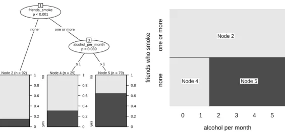
The classification tree derived from the smoking data is illustrated in Figure 1 (left) and shows the following: From the entire sample of 200 adolescents (represented by node 1 in Figure1(left), where the node numbers are mere labels assigned recursively from left to right starting from the top node), a group of 92 adolescents is separated from the rest in the first split. This group (represented by node 2) is characterized by the fact that “none” of their four best friends smoke, and that within this group only few subjects intend to smoke within the next year. The remaining 108 subjects are further split into two groups (nodes 4 and 5) according to whether they drank alcohol in “one or less” or “more” occasions in the past month. These two groups again vary in the percentage of subjects who intend to smoke.
The model can be displayed either as a tree, as in Figure1(left), or as a rectangular partition of the feature space, as in Figure 1(right): The first split in the variablefriends_smokepartitions the entire sample, while the second split in the variable alcohol_per_month further partitions only those subjects whose value for the variable friends_smokeis ”one or more”. The partition representation in Figure1(right) is even better suited than the tree representation to illustrate that recursive partitioning creates nested rectangular prediction areas corresponding to the terminal nodes of the classification tree. Details about the prediction rules derived from the partition are given below.
Note that the resulting partition is one of the main differences between classification trees and, e.g., linear regression models: While in linear regression the information from different predictor variables is combined linearly, here the range of possible combinations includes all rectangular partitions that can be derived by means of recursive splitting – including multiple splits in the same variable. In particular, this includes nonlinear and even nonmonotone association rules, that do not need to be specified in advance but are determined in a data driven way.
Of course there is a strong parallel between tree building and stepwise regression, where predictors are also included one at a time in successive order. However, in stepwise linear regression the pre-dictors still have a linear effect on the dependent variable, while extensions of stepwise procedures including interaction effects are typically limited to the inclusion of two-fold interactions, since the number of higher order interactions – that would have to be created simultaneously when starting the selection procedure – is too large.
In contrast to this, in recursive partitioning only those interactions that are actually used in the tree are generated during the fitting process. The issue of including main effects and interactions
in recursive partitioning is discussed in more detail below.
friends_smoke p < 0.001
1
none one or more
Node 2 (n = 92) yes no 0 0.2 0.4 0.6 0.8 1 alcohol_per_month p = 0.039 3 ≤≤1 >>1 Node 4 (n = 29) yes no 0 0.2 0.4 0.6 0.8 1 Node 5 (n = 79) yes no 0 0.2 0.4 0.6 0.8 1
alcohol per month
friends who smoke
none one or more 0 1 2 3 4 5 Node 5 Node 4 Node 2
Figure 1: Partition of the smoking data by means of a binary classification tree. The tree representation (left) corresponds to a rectangular recursive partition of the feature space (right). In the terminal nodes of the tree, the dark and light grey shaded areas represent the relative frequencies of “yes” and ”no” answers to the intention to smoke question in each group respectively. The corresponding areas in the rectangular partition are shaded in the color of the majority response.
Splitting and Stopping
Both the CART algorithm of Breiman et al. (1984) and the C4.5 algorithm (and its predecessor ID3) ofQuinlan (1986,1993) conduct binary splits in numeric predictor variables, as depicted in Figure 1. In categorical predictor variables (of nominal or ordinal scale of measurement) C4.5 produces as many nodes as there are categories (often referred to as “k-ary” or “multiple” split-ting), while CART again creates binary splits between the ordered or unordered categories. We concentrate on binary splitting trees in the following and refer toQuinlan(1993) fork-ary splitting. For selecting the splitting variable and cutpoint, both CART and C4.5 follow the approach of impurity reduction, that we will illustrate by means of our smoking data example: In Figure 2
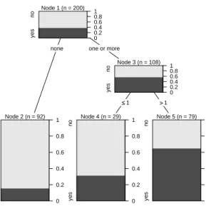
the relative frequencies of both response classes are displayed not only for the terminal nodes, but also for the inner nodes of the tree previously presented in Figure1. Starting from the root node, we find that the relative frequency of “yes” answers in the entire sample of 200 adolescents is approximately 40%. By means of the first split, the group of 92 adolescents with the lowest frequency of “yes” answers (approximately 15%, node 2) can be isolated from the rest, that have a higher frequency of “yes” answers (almost 60%, node 3). These 108 subjects are then further split to form two groups: one smaller group with a medium (approximately 30%, node 4) and one larger group with a high (more than 60%, node 5) frequency of “yes” answers to the intention to smoke question.
Node 1 (n = 200) yes no 0 0.2 0.4 0.6 0.8 1
none one or more
Node 2 (n = 92) yes no 0 0.2 0.4 0.6 0.8 1 Node 3 (n = 108) yes no 0 0.2 0.4 0.6 0.8 1 ≤≤1 >>1 Node 4 (n = 29) yes no 0 0.2 0.4 0.6 0.8 1 Node 5 (n = 79) yes no 0 0.2 0.4 0.6 0.8 1
Figure 2: Relative frequencies of both response classes in the inner nodes of the binary classification tree for the smoking data. The dark and light grey shaded areas again represent the relative frequencies of “yes” and ”no” answers to the intention to smoke in each group respectively.
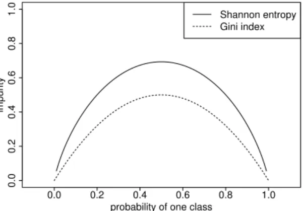
From this example we can see that, following the principle of impurity reduction, each split in the tree building process results in daughter nodes that are more ”pure” than the parent node in the sense that groups of subjects with a majority for either response class are isolated. The impurity reduction achieved by a split is measured by the difference between the impurity in the parent node and the average impurity in the two daughter nodes. Entropy measures, such as the Gini Index or the Shannon Entropy, are used to quantify the impurity in each node. These entropy measure have in common that they reach their minimum for perfectly pure nodes with the relative frequency of one response class being zero and their maximum for an equal mixture with the same relative frequencies for both response classes, as illustrated in Figure3.
While the principle of impurity reduction is intuitive and has added much to the popularity of classification trees, it can help our statistical understanding to think of impurity reduction as merely one out of many possible means of measuring the strength of the association between the splitting variable and the response. Most modern classification tree algorithms rely on this strategy, and employ the p-values of association tests for variable and cutpoint selection. This approach has additional advantages over the original impurity reduction approach, as outlined below.
Regardless of the split selection criterion, however, in each node the variable that is most strongly associated with the response variable (i.e., that produces the highest impurity reduction or the lowest p-value) is selected for the next split. In splitting variables with more than two categories, that offer more than one possible cutpoint, the optimal cutpoint is also selected with respect to this criterion. In our example, the optimal cutpoint identified within the range of the numeric
0.0 0.2 0.4 0.6 0.8 1.0 0.0 0.2 0.4 0.6 0.8 1.0
probability of one class
impurity
Shannon entropy Gini index
Figure 3: Gini index and Shannon entropy as functions of the relative frequency of one response class. Pure nodes containing only observations of one class receive an impurity value of zero, while mixed nodes receive higher impurity values.
predictor variablealcohol_per_monthis between the values 1 and 2, because subjects who drank alcohol in one or less occasions have a lower frequency of “yes” answers than those who drank alcohol in 2 or more occasions.
After a split is conducted, the observations in the learning sample are divided into the different nodes defined by the respective splitting variable and cutpoint, and in each node splitting continues recursively until some stop condition is reached. Common stop criteria are: split until (a) all leaf nodes are pure (i.e. contain only observations of one class) (b) a given threshold for the minimum number of observations left in a node is reached or (c) a given threshold for the minimum change in the impurity measure is not succeeded any more by any variable. Recent classification tree algorithms also provide statistical stopping criteria that incorporate the distribution of the splitting criterion (Hothorn, Hornik, and Zeileis 2006), while early algorithms relied on pruning the complete tree to avoid overfitting.
The term overfitting refers to the fact that a classifier that adapts too closely to the learning sample will not only discover the systematic components of the structure that is present in the population, but also the random variation from this structure that is present in the learning data due to random sampling. When such an overfitted model is later applied to a new test sample from the same population, its performance will be poor because it does not generalize well. However, it should be noted that overfitting is an equally relevant issue in parametric models: With every variable, and thus every parameter, that is added to the regression model, its fit to the learning data improves, because the model becomes more flexible.
This is evident, e.g., in theR2 statistic reflecting the portion of variance explained by the model, that increases with every parameter added to the model. For example, in the extreme case where as many parameters as observations are available, any parametric model will show a perfect fit on the learning data, yielding a value ofR2= 1, but will perform poorly in future samples.
variable selection in regression models. However, one should be aware that in this case significance tests do not work in the same way as in a designed study, where a limited number of hypotheses to be tested are specified in advance. In common forward and/or backward stepwise regression it is not known beforehand how many significance tests will have to be conducted. Therefore, it is hard to control the overall significance level, that controls the probability of falsely declaring at least one of the coefficients as significant.
Advanced variable selection strategies, that have been developed for parametric models, employ model selection criteria such as the AIC and BIC, that include a penalization term for the number of parameters in the model. For a detailed discussion of approaches that account for the complexity of parametric models seeBurnham and Anderson(2002) orBurnham and Anderson(2004). Since information criteria such as the AIC and BIC are, however, not applicable to nonparametric models (see, e.g.,Claeskens and Hjort 2008), in recursive partitioning the classic strategy to cope with overfitting is to “prune” the trees after growing them, which means that branches that do not add to the prediction accuracy in cross validation are eliminated. Pruning is not discussed in detail here, because the unbiased classification tree algorithm ofHothorn et al.(2006), that is used here for illustration, employs p-values for variable selection and as a stopping criterion and therefore does not rely on pruning. In addition to this, ensemble methods, that are our main focus here, usually employ unpruned trees.
Prediction and Interpretation of Classification and Regression Trees
Finally a response class is predicted in each terminal node of the tree (or each rectangular section in the partition respectively) by means of deriving from all observations in this node either the average response value in regression or the most frequent response class in classification trees. Note that this means that a regression tree creates a piecewise (or rectangle-wise for two dimensions and cuboid-wise in higher dimensions) constant prediction function.
Even though the idea of piecewise constant functions may appear very inflexible, such functions can be used to approximate any functional form, in particular nonlinear and nonmonotone functions. This is in strong contrast to classical linear or additive regression, where the effects of predictors are restricted to the additive form – the interpretation of which may appear easier, but which may also produce severe artifacts, since in many complex applications the true data generating mechanism is neither linear nor additive. We will see later that ensemble methods, by combining the predictions of many single trees, can approximate functions more smoothly, too.
The predicted response classes in our example are the majority class in each node in Figure 1
(left), as indicated by the shading in Figure1 (right): Subjects who have not lied to their parents as well as those who have lied to their parents but drank alcohol in one or less occasions are not likely to intend to smoke, while those who have lied to their parents and drank alcohol in 2 or more occasions are likely to intend to smoke within the next year.
For classification problems it is also possible to predict an estimate of the class probabilities from the relative frequencies of each class in the terminal nodes. In our example, the predicted probabilities for answering “yes” to the intention to smoke question would thus be approximately
friends_smoke p < 0.001
1
none one or more alcohol_per_month p < 0.001 2 ≤≤1 >>1 Node 3 yes no 0 0.2 0.4 0.6 0.8 1 Node 4 yes no 0 0.2 0.4 0.6 0.8 1 alcohol_per_month p < 0.001 5 ≤≤1 >>1 Node 6 yes no 0 0.2 0.4 0.6 0.8 1 Node 7 yes no 0 0.2 0.4 0.6 0.8 1 friends_smoke p < 0.001 1
none one or more alcohol_per_month p < 0.001 2 ≤≤1 >>1 Node 3 yes no 0 0.2 0.4 0.6 0.8 1 Node 4 yes no 0 0.2 0.4 0.6 0.8 1 alcohol_per_month p < 0.001 5 ≤≤1 >>1 Node 6 yes no 0 0.2 0.4 0.6 0.8 1 Node 7 yes no 0 0.2 0.4 0.6 0.8 1
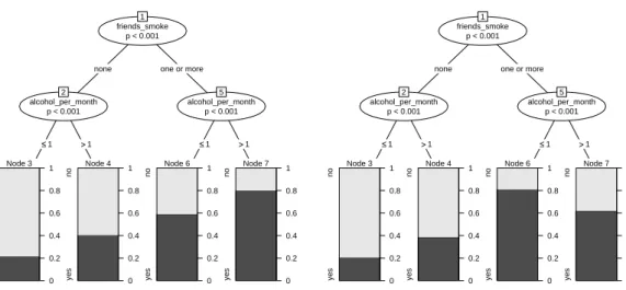
Figure 4: Classification trees based on variations of the smoking data with two main effects (left) and interactions (right). The tree depicted in Figure1based on the original data also represents an interaction.
15%, 30% and 65% in the three groups – which may preserve more information than the majority vote that merely assigns the class with a relative frequency of>50% as the prediction.
Reporting the predicted class probabilities more closely resembles the output of logistic regression models and can also be employed for estimating treatment probabilities or propensity scores. Note, however, that no confidence intervals are available for the estimates, unless, e.g., bootstrapping is used in combination with refitting to assess the variability of the prediction.
The easy interpretability of the visual representation of classification trees, that we have illustrated in this example, has added much to the popularity of this method, e.g., in medical applications. However, the downside of this apparently straightforward interpretability is that the visual repre-sentation may be misguiding, because the actual statistical interpretation of a tree model is not trivial. Especially the notions of main effects and interactions are often used rather incautiously in the literature, as seems to be the case inBerk(2006, p. 272), where it is stated that a branch that is not split any further indicated a main effect. However, when in the other branch created by the same variable splitting continues, as is the case in the example ofBerk(2006), this statement is not correct.
The term “interaction” commonly describes the fact that the effect of one predictor variable, in our example alcohol_per_month, on the response depends on the value of another predictor variables, in our examplefriends_smoke. For classification trees this means that, if in one branch created by friends_smokeit is not necessary to split in alcohol_per_month, while in the other branch created by friends_smoke it is necessary, as in Figure 1 (left), an interaction between friends_smokeandalcohol_per_monthis present.
We will further illustrate this important issue and source of misinterpretations by means of varying the effects in our artificial data set. The resulting classification trees are given in Figure4. Only
the left plot in Figure4, where the effect of alcohol_per_monthis the same in both branches cre-ated byfriends_smoke, represents two main effects of alcohol_per_month andfriends_smoke without an interaction: The main effect of friends_smokeshows in the higher relative frequen-cies of “yes” answers in nodes 6 and 7 as compared to nodes 3 and 4. The main effect of al-cohol_per_month shows in the higher relative frequencies of “yes” answers in nodes 4 and 7 as compared to nodes 3 and 6 respectively.
As opposed to that, both the right plot in Figure 4 and the original plot in Figure 1 represent interactions, because the effect of alcohol_per_month is different in both branches created by friends_smoke. In the right plot in Figure4the same split inalcohol_per_monthis conducted in every branch created byfriends_smoke, but the effect on the relative frequencies of the response classes is different: for those subjects who have no friends that smoke, the relative frequency of a “yes” answer is higher if they drank alcohol in 2 or more occasions (node 4 as compared to node 3), while for those who have one or more friends that smoke, the frequency of a “yes” answer is lower if they drank alcohol in 2 or more occasions (node 7 as compared to node 6). This example represents a typical interaction effect as known from standard statistical models, where the effect of alcohol_per_monthdepends on the value of friends_smoke.
In the original plot in Figure1on the other hand, the effect ofalcohol_per_monthis also different in both branches created by friends_smoke, because alcohol_per_month has an effect only in the right branch, but not in the left branch.
While this kind of “asymmetric” interaction is very common in classification trees, it is extremely unlikely to actually discover a symmetric interaction pattern as that in Figure4(right) or even a main effect pattern as that in Figure4(left) in real data.
The reason for this is that, even if the true distribution of the data in both branches was very similar, due to random variations in the sample and the deterministic variable and cutpoint selec-tion strategy of classificaselec-tion trees, it is extremely unlikely that the same splitting variable – and also the exact same cutpoint – would be selected in both branches. However, even a slightly dif-ferent cutpoint in the same variable would, strictly speaking, represent an interaction. Therefore it is stated in the literature that classification trees cannot (or rather, are extremely unlikely to) represent additive functions that consist only of main effects, while they are perfectly well suited for representing complex interactions.
For exploratory data analysis, further means for illustrating the effects of particular variables in classification trees are provided by the partial dependence plots described in Hastie, Tibshirani,
and Friedman(2001,2009) and the CARTscans toolbox (Nason, Emerson, and Leblanc 2004).
Model-Based Recursive Partitioning
A variant of recursive partitioning, that can also be a useful aid for visual data exploration, is model based recursive partitioning. Here the idea is to partition the feature space not such as to identify groups of subjects with similar values of the response variable, but groups of subjects with similar association patterns, e.g., between another predictor variable and the response. For example, linear regression could be used to model the dependence of a clinical response on
the dose of medication. However, the slope and intersect parameters of this regression may be different for different groups of patients: elderly patients, e.g., may show a stronger reaction to the medication, so that the slope of their regression line would need to be steeper than that of younger patients. In this example, the model of interest is the regression between dose of medication and clinical response – however, the model parameters should be chosen differently in the two (or more) groups defined by the covariate age. Another example and visualization are given in the section “Further application examples”.
The model based recursive partitioning approach of Zeileis, Hothorn, and Hornik (2008) offers a way to partition the feature space in order to detect parameter instabilities in the parametric model of interest by means of a structural change test framework. Similarly to latent class or mixture models, the aim of model based partitioning is to identify groups of subjects for which the parameters of the parametric model differ. However, in model based partitioning the groups are usually not defined by a latent factor, but by combinations of observed covariates, that are searched heuristically. Thus, model based partitioning can offer a heuristic but easy to interpret alternative to latent class – as well as random or mixed effects – models.
An extension of model based partitioning for Bradley-Terry models is suggested byStrobl,
Wick-elmaier, and Zeileis (2009). An application to mixed models, including the Rasch Model as a
special case (as a generalized linear mixed model, see Rijmen, Tuerlinckx, Boeck, and Kuppens
2003;Doran, Bates, Bliese, and Dowling 2007), is currently investigated bySanchez-Espigares and
Marco(2008).
What is Wrong with Trees?
The main flaw of simple tree models is their instability to small changes in the learning data: In recursive partitioning, the exact position of each cutpoint in the partition, as well as the decision which variable to split in, determines how the observations are split up in new nodes, in which splitting continues recursively. However, the exact position of the cutpoint, as well as the selection of the splitting variable, strongly depend on the particular distribution of observations in the learning sample.
Thus, as an undesired side effect of the recursive partitioning approach, the entire tree structure could be altered if the first splitting variable, or only the first cutpoint, was chosen differently due to a small change in the learning data. Due to this instability, the predictions of single trees show a high variability.
The high variability of single trees can be illustrated, e.g., by drawing bootstrap samples from the original data set and investigating whether the trees built on the different samples have a different structure. The rationale of bootstrap samples, where a sample of the same size as the original sample is drawn with replacement (so that some observations are left out, while others may appear more than once in the bootstrap sample) is to reflect the variability inherent in any sampling process: Random sampling preserves the systematic effects present in the original sample or population, but in addition to this it induces random variability. Thus, if classification trees built on different bootstrap samples vary too strongly in their structure, this proves that their
friends_smoke p < 0.001
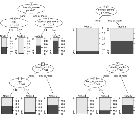
1
none one or more age p = 0.02 2 ≤≤12 >>12 Node 3 yes no 0 0.2 0.4 0.6 0.8 1 Node 4 yes no 0 0.2 0.4 0.6 0.8 1 alcohol_per_month p = 0.015 5 ≤≤4 >>4 Node 6 yes no 0 0.2 0.4 0.6 0.8 1 Node 7 yes no 0 0.2 0.4 0.6 0.8 1 friends_smoke p < 0.001 1
none one or more age p = 0.003 2 ≤≤12 >>12 Node 3 yes no 0 0.2 0.4 0.6 0.8 1 Node 4 yes no 0 0.2 0.4 0.6 0.8 1 Node 5 yes no 0 0.2 0.4 0.6 0.8 1 friends_smoke p < 0.001 1
none one or more Node 2 yes no 0 0.2 0.4 0.6 0.8 1 Node 3 yes no 0 0.2 0.4 0.6 0.8 1 friends_smoke p < 0.001 1
none one or more lied_to_parents p = 0.042 2 no yes Node 3 yes no 0 0.2 0.4 0.6 0.8 1 Node 4 yes no 0 0.2 0.4 0.6 0.8 1 Node 5 yes no 0 0.2 0.4 0.6 0.8 1
Figure 5: Classification trees based on four bootstrap samples of the smoking data, illus-trating the instability of single trees.
interpretability can be severely affected by the random variability present in any data set. Classification trees built on four bootstrap samples drawn from our original smoking data are displayed in Figure5. Apparently, the effect of the variablefriends_smokeis strong enough to remain present in all four trees, while the further splits vary strongly with the sample.
As a solution to the problem of instability, the average over an ensembles of trees, rather than a single tree, is used for prediction in ensemble methods, as outlined in the following. Another problem of single trees, that is solved by the same model averaging approach, is that the prediction of single trees is piecewise constant and thus may “jump” from one value to the next even for small changes of the predictor values. As described in the next section, ensemble methods have the additional advantage, that their decision boundaries are more smooth than those of single trees.
How Do Ensemble Methods Work?
The rationale behind ensemble methods is to base the prediction on a whole set of classification or regression trees, rather than a single tree. The related methods bagging and random forests vary only in the way this set of trees is constructed.
friends_smoke p < 0.001
1
none one or more lied_to_parents p = 0.061 2 no yes Node 3 yes no 0 0.2 0.4 0.6 0.8 1 age p = 0.536 4 ≤≤12 >>12 Node 5 yes no 0 0.2 0.4 0.6 0.8 1 age p = 0.362 6 ≤≤13>>13 Node 7 yes no 0 0.2 0.4 0.6 0.8 1 Node 8 yes no 0 0.2 0.4 0.6 0.8 1 age p = 0.081 9 ≤≤13 >>13 alcohol_per_month p = 0.186 10 ≤≤1 >>1 Node 11 yes no 0 0.2 0.4 0.6 0.8 1 lied_to_parents p = 0.352 12 yes no alcohol_per_month p = 0.402 13 ≤≤3 >>3 Node 14 yes no 0 0.2 0.4 0.6 0.8 1 Node 15 yes no 0 0.2 0.4 0.6 0.8 1 Node 16 yes no 0 0.2 0.4 0.6 0.8 1 lied_to_parents p = 0.214 17 no yes Node 18 yes no 0 0.2 0.4 0.6 0.8 1 Node 19 yes no 0 0.2 0.4 0.6 0.8 1 friends_smoke p < 0.001 1
none one or more lied_to_parents p = 0.076 2 no yes Node 3 yes no 0 0.2 0.4 0.6 0.8 1 age p = 0.416 4 ≤≤12 >>12 Node 5 yes no 0 0.2 0.4 0.6 0.8 1 alcohol_per_month p = 0.408 6 ≤≤4 >>4 age p = 0.106 7 ≤≤14>>14 Node 8 yes no 0 0.2 0.4 0.6 0.8 1 Node 9 yes no 0 0.2 0.4 0.6 0.8 1 Node 10 yes no 0 0.2 0.4 0.6 0.8 1 alcohol_per_month p = 0.014 11 ≤≤1 >>1 Node 12 yes no 0 0.2 0.4 0.6 0.8 1 age p = 0.246 13 ≤≤15 >>15 lied_to_parents p = 0.758 14 no yes Node 15 yes no 0 0.2 0.4 0.6 0.8 1 age p = 0.744 16 ≤≤12>>12 Node 17 yes no 0 0.2 0.4 0.6 0.8 1 Node 18 yes no 0 0.2 0.4 0.6 0.8 1 Node 19 yes no 0 0.2 0.4 0.6 0.8 1 friends_smoke p < 0.001 1
one or more none lied_to_parents p = 0.192 2 no yes alcohol_per_month p = 0.094 3 ≤≤2 >>2 Node 4 yes no 0 0.2 0.4 0.6 0.8 1 Node 5 yes no 0 0.2 0.4 0.6 0.8 1 age p = 0.39 6 ≤≤13 >>13 alcohol_per_month p = 0.519 7 ≤≤1 >>1 Node 8 yes no 0 0.2 0.4 0.6 0.8 1 age p = 0.354 9 ≤≤12>>12 Node 10 yes no 0 0.2 0.4 0.6 0.8 1 Node 11 yes no 0 0.2 0.4 0.6 0.8 1 Node 12 yes no 0 0.2 0.4 0.6 0.8 1 lied_to_parents p = 0.059 13 no yes Node 14 yes no 0 0.2 0.4 0.6 0.8 1 age p = 0.237 15 ≤≤12 >>12 Node 16 yes no 0 0.2 0.4 0.6 0.8 1 alcohol_per_month p = 0.534 17 ≤≤4 >>4 age p = 0.393 18 ≤≤14>>14 Node 19 yes no 0 0.2 0.4 0.6 0.8 1 Node 20 yes no 0 0.2 0.4 0.6 0.8 1 Node 21 yes no 0 0.2 0.4 0.6 0.8 1 friends_smoke p < 0.001 1
one or more none alcohol_per_month p = 0.042 2 ≤≤1 >>1 Node 3 yes no 0 0.2 0.4 0.6 0.8 1 age p = 0.032 4 ≤≤14 >>14 age p = 0.425 5 ≤≤12 >>12 Node 6 yes no 0 0.2 0.4 0.6 0.8 1 Node 7 yes no 0 0.2 0.4 0.6 0.8 1 Node 8 yes no 0 0.2 0.4 0.6 0.8 1 lied_to_parents p = 0.053 9 no yes Node 10 yes no 0 0.2 0.4 0.6 0.8 1 age p = 0.268 11 ≤≤12 >>12 Node 12 yes no 0 0.2 0.4 0.6 0.8 1 age p = 0.533 13 ≤≤13 >>13 Node 14 yes no 0 0.2 0.4 0.6 0.8 1 Node 15 yes no 0 0.2 0.4 0.6 0.8 1
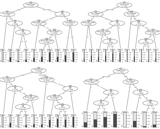
Figure 6: Classification trees (grown without stopping or pruning) based on four bootstrap samples of the smoking data, illustrating the principle of bagging.
Bagging
In both bagging and random forests a set of trees is built on random samples of the learning sample: In each step of the algorithm, either a bootstrap sample (of the same size, drawn with replacement) or a subsample (of smaller size, drawn without replacement) of the learning sample is drawn randomly, and an individual tree is grown on each sample. As outlined above, each random sample reflects the same data generating process but differs slightly from the original learning sample due to random variation. Keeping in mind that each individual classification tree depends highly on the learning sample as outlined above, the resulting trees can thus differ substantially. Another feature of the ensemble methods bagging and random forests is that usually trees are grown very large, without any stopping or pruning involved. As illustrated again for four bootstrap samples from the smoking data in Figure6, large trees can become even more diverse and include a large variety of combinations of predictor variables.
By combining the prediction of such a diverse set of trees, ensemble methods utilize the fact that classification trees are instable but on average produce the right prediction (i.e. trees are unbiased
predictors), which has been supported by several empirical as well as simulation studies (cf., e.g.,
Breiman 1996a, 1998; Bauer and Kohavi 1999; Dietterich 2000) and especially the theoretical
results ofB¨uhlmann and Yu (2002), that show the superiority in prediction accuracy of bagging over single classification or regression trees: B¨uhlmann and Yu (2002) could show by means of rigorous asymptotic methods that the improvement in the prediction is achieved by means of smoothing the hard cut decision boundaries created by splitting in single classification trees, which in return reduces the variance of the prediction (see also Biau, Devroye, and Lugosi 2008). The smoothing of hard decision boundaries also makes ensembles more flexible than single trees in approximating functional forms that are smooth rather than piecewise constant.
Grandvalet(2004) also points out that the key effect of bagging is that it equalizes the influence
of particular observations – which proves beneficial in the case of “bad” leverage points, but may be harmful when “good” leverage points, that could improve the model fit, are downweighted. The same effect can be achieved not only by means of bootstrap sampling as in standard bagging, but also by means of subsampling (Grandvalet 2004), that is preferable in many applications because it guarantees unbiased variable selection (Strobl, Boulesteix, Zeileis, and Hothorn 2007, see also section “Bias in variable selection and variable importance”). Ensemble construction can also be viewed in the context of Bayesian model averaging (cf., e.g., Domingos 1997;Hoeting, Madigan,
Raftery, and Volinsky 1999, for an introduction). For random forests, which we will consider in the
next section,Breiman(2001a, p. 25) states that they may also be viewed as a Bayesian procedure (and continues: “Although I doubt that this is a fruitful line of exploration, if it could explain the bias reduction, I might become more of a Bayesian.”).
Random Forests
In random forests another source of diversity is introduced when the set of predictor variables to select from is randomly restricted in each split, producing even more diverse trees. The number of randomly preselected splitting variables, termedmtryin most algorithms, as well as the overall number of trees, usually termedntree, are parameters of random forests that affect the stability of the results and will be discussed further in section “Features and pitfalls”. Obviously random forests include bagging as the special case where the number of randomly preselected splitting variables is equal to the overall number of variables.
Intuitively speaking, random forests can improve the predictive performance even further as com-pared to bagging, because the single trees involved in averaging are even more diverse. From a statistical point of view, this can be explained by the theoretical results presented by Breiman
(2001a), that the upper bound for the generalization error of an ensemble depends on the
correla-tion between the individual trees, such that a low correlacorrela-tion between the individual trees results in a low upper bound for the error.
In addition to the smoothing of hard decision boundaries, the random selection of splitting vari-ables in random forests allows predictor varivari-ables, that were otherwise outplayed by a stronger competitor, to enter the ensemble: If the stronger competitor cannot be selected, a new variable has a chance to be included in the model – and may reveal interaction effects with other variables that otherwise would have been missed.
lied_to_parents p = 0.22 1 no yes alcohol_per_month p = 0.217 2 ≤≤2 >>2 Node 3 yes no 0 0.2 0.4 0.6 0.8 1 Node 4 yes no 0 0.2 0.4 0.6 0.8 1 alcohol_per_month p = 0.685 5 ≤≤4 >>4 friends_smoke p = 0.01 6
none one or more age p = 0.652 7 ≤≤12 >>12 Node 8 yes no 0 0.2 0.4 0.6 0.8 1 age p = 0.17 9 ≤≤14 >>14 Node 10 yes no 0 0.2 0.4 0.6 0.8 1 Node 11 yes no 0 0.2 0.4 0.6 0.8 1 age p = 0.103 12 ≤≤12 >>12 Node 13 yes no 0 0.2 0.4 0.6 0.8 1 alcohol_per_month p = 0.696 14 ≤≤1 >>1 Node 15 yes no 0 0.2 0.4 0.6 0.8 1 Node 16 yes no 0 0.2 0.4 0.6 0.8 1 friends_smoke p = 0.025 17
noneone or more
Node 18 yes no 0 0.2 0.4 0.6 0.8 1 Node 19 yes no 0 0.2 0.4 0.6 0.8 1 friends_smoke p < 0.001 1
none one or more age p = 0.111 2 ≤≤12 >>12 Node 3 yes no 0 0.2 0.4 0.6 0.8 1 alcohol_per_month p = 0.173 4 ≤≤4 >>4 age p = 0.25 5 ≤≤14 >>14 Node 6 yes no 0 0.2 0.4 0.6 0.8 1 Node 7 yes no 0 0.2 0.4 0.6 0.8 1 Node 8 yes no 0 0.2 0.4 0.6 0.8 1 lied_to_parents p = 0.156 9 no yes alcohol_per_month p = 0.135 10 ≤≤3 >>3 Node 11 yes no 0 0.2 0.4 0.6 0.8 1 Node 12 yes no 0 0.2 0.4 0.6 0.8 1 age p = 0.143 13 ≤≤13 >>13 age p = 0.892 14 ≤≤12 >>12 Node 15 yes no 0 0.2 0.4 0.6 0.8 1 Node 16 yes no 0 0.2 0.4 0.6 0.8 1 Node 17 yes no 0 0.2 0.4 0.6 0.8 1 alcohol_per_month p = 0.016 1 ≤≤3 >>3 lied_to_parents p = 0.485 2 yes no alcohol_per_month p = 0.525 3 ≤≤0 >>0 Node 4 yes no 0 0.2 0.4 0.6 0.8 1 friends_smoke p = 0.028 5 none one or more age p = 0.991 6 ≤≤12 >>12 Node 7 yes no 0 0.2 0.4 0.6 0.8 1 age p = 0.31 8 ≤≤13 >>13 Node 9 yes no 0 0.2 0.4 0.6 0.8 1 Node 10 yes no 0 0.2 0.4 0.6 0.8 1 Node 11 yes no 0 0.2 0.4 0.6 0.8 1 Node 12 yes no 0 0.2 0.4 0.6 0.8 1 age p = 0.729 13 ≤≤12 >>12 Node 14 yes no 0 0.2 0.4 0.6 0.8 1 friends_smoke p = 0.003 15
noneone or more
Node 16 yes no 0 0.2 0.4 0.6 0.8 1 Node 17 yes no 0 0.2 0.4 0.6 0.8 1 lied_to_parents p = 0.154 1 yes no friends_smoke p < 0.001 2
none one or more age p = 0.955 3 ≤≤13 >>13 age p = 0.251 4 ≤≤12 >>12 Node 5 yes no 0 0.2 0.4 0.6 0.8 1 Node 6 yes no 0 0.2 0.4 0.6 0.8 1 age p = 0.321 7 ≤≤15>>15 Node 8 yes no 0 0.2 0.4 0.6 0.8 1 Node 9 yes no 0 0.2 0.4 0.6 0.8 1 age p = 0.128 10 ≤≤13 >>13 alcohol_per_month p = 0.017 11 ≤≤1 >>1 Node 12 yes no 0 0.2 0.4 0.6 0.8 1 alcohol_per_month p = 0.092 13 ≤≤2 >>2 Node 14 yes no 0 0.2 0.4 0.6 0.8 1 Node 15 yes no 0 0.2 0.4 0.6 0.8 1 Node 16 yes no 0 0.2 0.4 0.6 0.8 1 friends_smoke p < 0.001 17
noneone or more
Node 18 yes no 0 0.2 0.4 0.6 0.8 1 Node 19 yes no 0 0.2 0.4 0.6 0.8 1
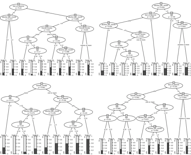
Figure 7: Classification trees (grown without stopping or pruning and with a random pres-election of 2 variables in each split) based on four bootstrap samples of the smoking data, illustrating the principle of random forests
The effect or randomly restricting the splitting variables is again illustrated by means of four bootstrap samples drawn from the smoking data: In addition to growing a large tree on each bootstrap sample, as in bagging, now the variable selection is limited tomtry=2 randomly prese-lected candidates in each split. The resulting trees are displayed in Figure7: We find that, due to the random restriction, the trees have become even more diverse; for example the strong predictor variablefriends_smokeis no longer chosen for the first split in every single tree.
The reason why even suboptimal splits in weaker predictor variables can often improve the pre-diction accuracy of an ensemble is that the split selection process in regular classification trees is only locally optimal in each node: A variable and cutpoint are chosen with respect to the impurity reduction they can achieve in a given node defined by all previous splits, but regardless of all splits yet to come.
Thus, variable selection in a single tree is affected by order effects similar to those present in step-wise variable selection approaches for parametric regression (that is also instable against random variation of the learning data, as pointed out byAustin and Tu 2004). In both recursive
partition-ing and stepwise regression, the approach of addpartition-ing one locally optimal variable at a time does not necessarily (or rather hardly ever) lead to the globally best model over all possible combinations of variables.
Since, however, searching for a single globally best tree is computationally infeasible (a first ap-proach involving dynamic programming was introduced byvan Os and Meulman 2005), the random restriction of the splitting variables provides an easy and efficient way to generate locally subopti-mal splits that can improve the global performance of an ensemble of trees. Alternative approaches that follow this rationale by introducing even more sources of randomness are outlined below. Besides intuitive explanations for “how ensemble methods work”, recent publications have con-tributed to a deeper understanding of the statistical background behind many machine learning methods: The work of B¨uhlmann and Yu (2002) provided the statistical framework for bagging,
Friedman, Hastie, and Tibshirani (2000) and B¨uhlmann and Yu (2003) for the related method
boosting and, most recently, Lin and Jeon (2006) andBiau et al. (2008) for random forests. In their work Lin and Jeon (2006) explore the statistical properties of random forests by means of placing them in a k-nearest neighbor (k-NN) framework, where random forests can be viewed as adaptively weighted k-NN with the terminal node size determining the size of neighborhood. However, in order to be able to mathematically grasp a computationally complex method like random forests, involving several degrees of random sampling, several simplifying assumptions are necessary. Therefore well planned simulation studies still offer valuable assistance for evaluating statistical aspects of the method in its original form.
Alternative Ensemble Methods
Alternative approaches for building ensembles of trees with a strong randomization component are the random split selection approach of Dietterich(2000), where cutpoints from a set of optimal candidates are randomly selected, and the perfect random trees approach of Cutler (1999) and
Cutler(2000), where both the splitting variable and the cutpoint are chosen randomly for each
split.
Another very intuitive approach, that resides somewhere in between single classification trees and the ensemble methods we have covered so far, is TWIX (Potapov 2007;Potapov, Theus, and
Urbanek 2006). Here the building of the tree ensemble starts in a single starting node but branches
to a set of trees at each decision by means of splitting not only in the best cutpoint but also in reasonable extra cutpoints. A data driven approach for selecting extra cutpoints is suggested in
Strobl and Augustin(2009).
However, while the approaches involving a strong randomization component manage to overcome local optimality as outlined above, the TWIX approach is limited to a sequence of locally optimal splits. It has been shown to outperform single trees and even to reach the predictive performance of bagging, but in general cannot compete because it becomes computationally infeasible for large sets of trees that are standard in today’s ensemble methods.
Predictions from Ensembles of Trees
In an ensemble of trees the predictions of all individual trees need to be combined. This is usually accomplished by means of (weighted or unweighted) averaging in regression or voting in classification.
The term “voting” can be taken literally here: Each subject with given values of the predictor variables is “dropped through” every tree in the ensemble, so that each single tree returns a predicted class for the subject. The class that most trees “vote” for is returned as the prediction of the ensemble. This democratic voting process is the reason why ensemble methods are also called “committee” methods. Note, however, that there is no diagnostic for the unanimity of the vote. For regression and for predicting probabilities, i.e. relative class frequencies, the results of the single trees are averaged; some algorithms also employ weighted averages. A summary over several aggregation schemes is given inGatnar(2008). However, even with the simple aggregation schemes used in the standard algorithms, ensembles methods reliably outperform single trees and many other advanced methods (examples of benchmark studies are given in the discussion). Aside from the issue of aggregation, for bagging and random forests there are two different pre-diction modes: ordinary prepre-diction and the so called out-of-bag prepre-diction. While in ordinary prediction each observation of the original data set – or a new test data set – is predicted by the entire ensemble, out-of-bag prediction follows a different rationale: Remember that each tree is built on a bootstrap sample, that serves as a learning sample for this particular tree. However, some observations, namely the out-of-bag observations, were not included in the learning sample for this tree. Therefore, they can serve as a “built-in” test sample for computing the prediction accuracy of that tree.
The advantage of the out-of-bag error is that it is a more realistic estimate of the error rate that is to be expected in a new test sample, than the naive and over-optimistic estimate of the error rate resulting from the prediction of the entire learning sample (Breiman 1996b) (see alsoBoulesteix,
Strobl, Augustin, and Daumer (2008) for a review on resampling-based error estimation). The
standard and out-of-bag prediction accuracy of a random forests with ntree=500 and mtry=2 for our smoking data example is 74.5% and 71.5% respectively, where the out-of-bag prediction accuracy is more conservative.
In our artificial example, bagging, and even a single tree, would actually perform equally well, because the interaction of friends_smoke and alcohol_per_month, that was already correctly identified by the single tree, is the only effect that was induced in the data.
However, in most real data applications – especially in cases where many predictor variables work in complex interactions – the prediction accuracy of random forests is found to be higher than for bagging, and both ensemble methods usually highly outperform single trees.
Variable Importance
As described in the previous sections, single classification trees are easily interpretable, both intuitively at first glance and descriptively when looking in detail at the tree structure. In particular variables that are not included in the tree did not contribute to the model – at least not in the
context of the previously chosen splitting variables.
As opposed to that, ensembles of trees are not easy to interpret at all, because the individual trees in them are not nested in any way: Each variable may appear at different positions, if at all, in different trees, as depicted in Figures6 and7, so that there is no such thing as an “average tree” that could be visualized for interpretation.
On the other hand, an ensemble of trees has the advantage that it gives each variable the chance to appear in different contexts with different covariates, and can thus better reflect its potentially complex effect on the response. Moreover, order effects induced by the recursive variable selection scheme employed in constructing the single trees are eliminated by averaging over the entire ensemble. Therefore, in bagging and random forests variable importance measures are computed to assess the relevance of each variable over all trees of the ensemble.
In principle, a possible naive variable importance measure would be to merely count the number of times each variable is selected by all individual trees in the ensemble. More elaborate variable importance measures incorporate a (weighted) mean of the individual trees’ improvement in the splitting criterion produced by each variable (Friedman 2001). An example for such a measure in classification is the “Gini importance” available in random forest implementations. It describes the average improvement in the “Gini gain” splitting criterion that a variable has achieved in all of its positions in the forest. However, in many applications involving predictor variables of different types, this measure is biased, as outlined in section “Bias in variable selection and variable importance”.
The most advanced variable importance measure available in random forests is the “permutation accuracy importance” measure (termed permutation importance in the following). Its rationale is the following: By randomly permuting the values of a predictor variable, its original association with the response is broken.
For example, in the original smoking data, those adolescents who drank alcohol in more occasions are more likely to intend to smoke. Randomly permuting the values of alcohol_per_month over all subjects, however, destroys this association. Accordingly, when the permuted variable, together with the remaining unpermuted predictor variables, is now used to predict the response, the prediction accuracy decreases substantially.
Thus, a reasonable measure for variable importance is the difference in prediction accuracy (i.e. the number of observations classified correctly; usually the out-of-bag prediction accuracy is used to compute the permutation importance) before and after permuting a variable, averaged over all trees.
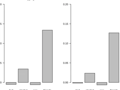
If, on the other hand, the original variable was not associated with the response, it is either not included in the tree (and its importance for this tree is zero by definition), or it is included in the tree by chance. In the latter case, permuting the variable results only in a small random decrease in prediction accuracy, or the permutation of an irrelevant variable can even lead to a small increase in the prediction accuracy (if, by chance, the permutated variable happens to be slightly better suited for splitting than the original one). Thus the permutation importance can even show (small) negative values for irrelevant predictor variables, as illustrated for the irrelevant
lied alcohol age friends bagging 0.00 0.05 0.10 0.15 0.20
lied alcohol age friends random forest 0.00 0.05 0.10 0.15 0.20
Figure 8: Permutation variable importance scores for the predictor variables of the smoking data from bagging and random forests.
predictor variablesageandlied_to_parents in Figure8.
Note also that in our simple example the two relevant predictor variables friends_smoke and alcohol_per_monthare correctly identified by the permutation variable importance of both bag-ging and random forests, even though the positions of the variables vary more strongly in random forests (cf. again Figures6 and7). In real data applications, however, the random forest variable importance may reveal higher importance scores for variables working in complex interactions, that may have gone unnoticed in single trees and bagging (as well as in parametric regression models, where modeling high-order interactions is usually not possible at all).
Formally the permutation importance for classification can be defined as follows: LetB(t) be the out-of-bag sample for a tree t, with t ∈ {1, . . . ,ntree}. Then the importance of variableXj in
treetis VI(t)(Xj) = P i∈B(t)I yi= ˆy (t) i B (t) − P i∈B(t)I yi= ˆy (t) i,ψj B (t) (1) where ˆyi(t) = f(t)(x
i) is the predicted class for observation i before and ˆy
(t)
i,ψj = f
(t)(x
i,ψj) is
the predicted class for observation i after permuting its value of variable Xj, i.e. with xi,ψj =
xi,1, . . . , xi,j−1, xψj(i),j, xi,j+1, . . . , xi,p
. (Note thatVI(t)(Xj) = 0 by definition, if variable Xj
is not in tree t.) The raw importance score for each variable is then computed as the average importance over all trees
VI(Xj) = Pntree t=1 VI (t)(X j) ntree . (2)
From this raw importance score a standardized importance score can be computed with the fol-lowing rationale: The individual importance scoresVI(t)(xj) are computed fromntreebootstrap
samples, that are independent given the original sample, and are identically distributed. Thus, if each individual variable importance VI(t) has standard deviation σ, the average importance from ntree replications has standard error σ/
√
ntree. The standardized or scaled importance,
also called “z-score”, is then computed as
z(xj) = VI(xj) ˆ σ √ ntree . (3)
When the central limit theorem is applied to the mean importance VI(xj), Breiman and Cutler
(2008) argue that thez-score is asymptotically standard normal. This property is often used for a statistical test, that, however, shows very poor statistical properties as outlined in the section on “Features and pitfalls”.
As already mentioned, the main advantage of the random forest permutation accuracy importance, as compared to univariate screening methods, is that it covers the impact of each predictor variable individually as well as in multivariate interactions with other predictor variables. For example
Lunetta et al. (2004) find that genetic markers relevant in interactions with other markers or
environmental variables can be detected more efficiently by means of random forests than by means of univariate screening methods like Fisher’s exact test.
This, together with its applicability to problems with many predictor values, also distinguishes the random forest variable importance from the otherwise appealing approach ofAzen, Budescu, and
Reiser(2001) and advanced inAzen and Budescu(2003) for assessing the criticality of a predictor
variable, termed “dominance analysis”: The authors suggest employing bootstrap sampling and select the best regression model from all possible models for each bootstrap sample in order to estimate the empirical probability distribution of all possible models. From this empirical distribution for each variable the unweighted or weighted sum of probabilities associated with all models containing the predictor is computed and suggested as an intuitive measure of variable importance. This approach, where for p predictor variables 2p−1 models are fitted in each
bootstrap iteration, has the great advantage that it provides sound statistical inference. However, it is computationally prohibitive for problems with many predictor variables of interest, because all possible models have to be fitted on all bootstrap samples.
In random forests, on the other hand, a tree model is fit to every bootstrap sample only once. Then the predictor variables are permuted in an attempt to mimic their absence in the prediction. This approach can be considered in the framework of classical permutation test procedures (Strobl,
Boulesteix, Kneib, Augustin, and Zeileis 2008) and is feasible for large problems, but lacks the
sound statistical background available for the approach ofAzen et al.(2001). Another difference is that random forest variable importances reflect the effect of a variable in complex interactions as outlined above, while the approach ofAzen et al.(2001) reflects the main effects – at least as long as interactions are not explicitly included in the candidate models.
A conditional version of the random forest permutation importance, that resembles the properties of partial correlations rather than that of dominance analysis, is suggested byStrobl et al.(2008).
Literature and Software
Random forests have only recently been included in standard textbooks on statistical learning, such
asHastie et al.(2009) (while the previous edition,Hastie et al. 2001, did not cover this topic yet).
In addition to a short introduction of random forests, this reference gives a thorough background on classification trees and related concepts of resampling and model validation, and is therefore highly recommended for further reading. For the social sciences audience a first instructive review on ensemble methods, including random forests and the related method bagging, was given by
Berk(2006). We suggest this reference for the treatment of unbalanced data (for example in the case of a rare disease or mental condition), that can be treated either by means of asymmetric misclassification costs or equivalently by means of weighting with different prior probabilities in classification trees and related methods (see alsoChen, Liaw, and Breiman 2004, for the alternative strategy of “down sampling”, i.e., sampling from the majority class as few observations as there are of the minority class), even though the interpretation of interaction effects in Berk(2006) is not coherent, as demonstrated above. The original works ofBreiman(1996a,b,1998,2001a,b), to name a few, are also well suited and not too technical for further reading.
For practical applications of the methods introduced here, several up-to-date tools for data analysis are freely available in theRsystem for statistical computing (RDevelopment Core Team 2008). Regarding this choice of software, we believe that the supposed disadvantage of command line data analysis criticized by Berk(2006) is easily outweighed by the advanced functionality of the
R language and its add-on packages at the state of the art of statistical research. However, in statistical computing the textbooks also lag behind the latest scientific developments: The standard referenceVenables and Ripley(2002) does not (yet) cover random forests either, while the handbook ofEveritt and Hothorn(2006) gives a short introduction to the use of both classification trees and random forests. This handbook, together with the instructive examples in the following section and theR-code provided in a supplement to this work, can offer a good starting point for applying random forests to your data. Interactive means of visual data exploration inR, that can support further interpretation, are described inCook and Swayne(2007).
Further Application Examples
For further illustration, two additional application examples of model based partitioning and random forests are outlined. The source code for reproducing all steps of the following analyses as well as the examples in the previous sections in the R system for statistical computing (R
Development Core Team 2009) is provided as a supplement.
Model-Based Recursive Partitioning
For a reaction time experiment, where the independent variable is sleep deprivation (subset of four exemplary subjects from the sleep-deprived group with measurements for the first 10 days of the study fromBelenky, Wesensten, Thorne, Thomas, Sing, Redmond, Russo, and Balkin 2003), it is illustrated in Figure 9 that the effect of sleep deprivation on reaction time differs between subjects.
Subject p < 0.001 1 {309, 335} {308, 350} Subject p < 0.001 2 309 335 Node 3 (n = 10) ● ● ● ● ● ● ● ● ● ● 0 9 177 492 Node 4 (n = 10) ● ● ● ● ● ● ● ● ● ● 0 9 177 492 Node 5 (n = 20) ● ● ● ● ● ● ● ● ● ● ● ● ● ● ● ● ● ● ● ● 0 9 177 492
Figure 9: Model-based partition for the reaction time data. The model of interest relates the number of days of sleep deprivation to the reaction time.
For each subject, the data set contains ten successive measurements (for days 0 through 9). The subject ID is used as a pseudo-covariate for model based partitioning here: The subject IDs are indicated in the tree structure in Figure 9, where the leftmost node, e.g., includes only the measurements of subject 309, while the rightmost node includes the measurements of subjects 308 and 350. The model of interest in each final node relates the number of days of sleep deprivation (0 through 9, on the abscissa) to the reaction time (on the ordinate).
We find that the reactions to sleep deprivation of subjects 308 and 350 can be represented by one joint model, while the reactions of the other subjects are represented by distinct models. If additional covariates, such as age and gender, rather than only the subject ID, were available for this study, they could be used for partitioning as well, while using the subject ID as a pseudo covariate as in this example resembles a latent class approach for identifying groups of subjects with similar response patterns.
Of course, differences between subjects or groups of subjects could also be modeled by means of, e.g., random effects or latent class models – but again the visual inspection of the model-based partition, that requires no further assumptions, can provide a helpful first glance impression of different response patterns present in the sample or help, e.g., identify groups of non-responders in clinical studies.
Random Forests
regression models are not applicable and ensemble methods are often applied for prediction and the assessment of variable importance.
For an exemplary analysis of gene data, we adopted a data set originally presented by Ryan,
Lockstone, Huffaker, Wayland, Webster, and Bahn (2006): The data were collected in a
case-control study on bipolar disorder including 61 samples (from 30 cases and 31 case-controls) from the dorsolateral prefrontal cortex cohort. In the original study of Ryan et al.(2006), no genes were clearly found to be differentially expressed, i.e., to have an effect on the disease, in this sample. Therefore, two genes were artificially modified to have an effect, so that we can later control whether these genes are correctly identified.
In order to be able to illustrate t’the variable importances in a plot, in addition to the two simulated genes and the three covariates age, gender and brain pH-level, a subset of 100 genes was randomly selected from the 22,283 genes originally present by Ryan et al. (2006) for the example. Note, however, that the application to larger data sets is only a question of computation time.
The permutation importances for all 105 variables are displayed in Figure 10. The effects of the two artificially modified genes can be clearly identified. With respect to the remaining variables, a conservative strategy for exploratory screening would be to include all genes whose importance scores exceed the amplitude of the largest negative scores (that can only be due to random varia-tion) in future studies.
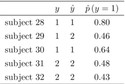
A prediction from the random forest can be given either in terms of the predicted response class or the predicted class probabilities, as illustrated in Table 1for some exemplary subjects, with a mismatch between the true and predicted class for subject 29.
Table 1: Predicted response class or class probability.
y yˆ pˆ(y= 1) subject 28 1 1 0.80 subject 29 1 2 0.46 subject 30 1 1 0.64 subject 31 2 2 0.48 subject 32 2 2 0.43
For the entire learning sample the prediction accuracy estimate is over-optimistic (90.16%), while the estimate based on the out-of-bag sample is more conservative (67.21%). The confusion matrices in Table2 display misclassifications separately for each response class.
Note that a logistic regression model would not be applicable in a sample of this size, even for the reduced data set with only 102 genes – not even if forward selection was employed and only main effects were considered, disregarding the possibility of interaction effects – because the estimation algorithm does not converge.
In other cases, however, the prediction accuracy of the complex random forests model, involving high-order interactions and nonlinearity, can be compared to that of a simpler, for example linear