Efficiency of accelerated coordinate descent method on structured optimization problems

Available at:

http://hdl.handle.net/2078.1/171232

"Efficiency of accelerated coordinate descent

method on structured optimization problems"

Nesterov, Yurii ; Stich, Sebastian

Abstract

In this paper we prove a new complexity bound for a variant of Accelerated

Coordinate Descent Method [7]. We show that this method often outperforms

the standard Fast Gradient Methods (FGM, [3, 6]) on optimization problems with

dense data. In many important situations, the computational expenses of oracle

and method itself at each iteration of our scheme are perfectly balanced (both

depend linearly on dimensions of the problem). As application examples, we

consider unconstrained convex quadratic minimization, and the problems arising

in Smoothing Technique [6]. On some special problem instances, the provable

acceleration factor with respect to FGM can reach the square root of the number

of variables. Our theoretical conclusions are confirmed by numerical experiments.

Document type : Document de travail (Working Paper)

Référence bibliographique

Nesterov, Yurii ; Stich, Sebastian.

Efficiency of accelerated coordinate descent method on

structured optimization problems. CORE Discussion Papers ; 2016/03 (2016) 20 pages

2016/03

!

Efficiency of accelerated coordinate descent method on

structured optimization problems

Yu. Nesterov and S. Stich

February 1, 2016

!

CORE

Voie du Roman Pays 34, L1.03.01

B-1348 Louvain-la-Neuve, Belgium.

Tel (32 10) 47 43 04

Fax (32 10) 47 43 01

CORE DISCUSSION PAPER

2016/03

Efficiency of accelerated coordinate descent method on

structured optimization problems

Yu. Nesterov

1

and S. Stich

2

February 1, 2016

Abstract

In this paper we prove a new complexity bound for a variant of Accelerated

Coordinate Descent Method [7]. We show that this method often outperforms

the standard Fast Gradient Methods (FGM, [3, 6]) on optimization problems

with dense data. In many important situations, the computational expenses of

oracle and method itself at each iteration of our scheme are perfectly balanced

(both depend linearly on dimensions of the problem). As application examples,

we consider unconstrained convex quadratic minimization, and the problems

arising in Smoothing Technique [6]. On some special problem instances, the

provable acceleration factor with respect to FGM can reach the square root of

the number of variables. Our theoretical conclusions are confirmed by

numerical experiments.

Keywords:

Convex optimization, structural optimization, fast gradient

methods, coordinate descent methods, complexity bounds

1 _{Center for Operations Research and Econometrics (CORE), Catholic University of Louvain}

(UCL), 34 voie du Roman Pays, 1348 Louvain-la-Neuve, Belgium.

2 _{CORE/ICTEAM (UCL). This research was supported by Swiss Science Foundation (SNF).}

The research results presented in this paper have been supported by a grant “Action de recherche concertée ARC 04/09-315” from the “Direction de la recherche scientifique - Communauté française de Belgique”. Scientific responsibility rests with the authors.

1

Introduction

Motivation.

In the last years, coordinate descent methods attract more and more

at-tention of the Optimization Community. Its popularity is based mainly on the fact that

they can be applied to problems of a very big size. Starting from the paper [7], it

be-came possible to provide the randomized variants of these schemes with very attractive

worst-case efficiency guarantees, which take into account a very high sparsity of the data.

Consequently, the further developments of these methods were naturally related to the

needs of Big-Data machinery: parallelization, distributed computing, etc (see, for

exam-ple, [4, 5]). However, in this paper we show that the coordinate descent strategies can be

useful even for the problems of moderate-size when the data is dense.

In [7], there was proposed a variant of Fast Gradient Method [3], where the gradient

step was replaced by a step along coordinate direction (we call this method Accelerated

Co-ordinate Descent Method, ACDM for short). It was suggested to choose the corresponding

active coordinate randomly, in accordance to uniform distribution. The expected

com-plexity of this scheme for finding an

!-solution for unconstrained minimization problem is

of the order

O

!

n !1/2

max

1≤i≤n

L

i

"

(1.1)

iterations, where

L

i

is the uniform upper bound on the

ith diagonal element of the Hessian

of the objective function, and

n

is the number of variables. At the same time, in [7] it was

also mentioned that this scheme is not appropriate for Huge-Scale optimization problems

since it needs at least one full-dimensional vector operation at each iteration.

Complexity bound (1.1) was improved in [2] up to the level

O

#$

n ! n

%

i=1

L

i

&

1/2

'

(1.2)

iterations. For choosing the active coordinate, the authors suggest to use probabilities

L

i

(

n

%

k₌₁

L

k

)

−1

,

i

= 1, . . . , n. Finally, in our paper we get the further improvement in the

complexity of ACDM, up to the level

O

!

1 !1/2 n

%

i=1

L

1_i/2

"

(1.3)

iterations. The probabilities we use now are defined as

L

1_i/2

(

n

%

k₌₁

L

1_k/2

)

−1

. This is the first

time when we get the complexity estimate of ACDM, which does not depend explicitly in

the dimension of the space of variables.

Another important result of our paper consists in finding interesting applications,

where the new scheme becomes dominant. We show that in

all

unconstrained convex

optimization problems obtained by Smoothing Technique [6], our method provably

out-performs the standard Fast Gradient Methods. For some classes of problems, the gain in

the computational time reaches the square root of the dimension. This improvement is

mainly achieved due to the fact, that in many situations the computational expenses at

each iteration of our method are perfectly balanced with the computational time spent

for updating the results of matrix-vector products (both depend linearly in the dimension

of the problem). For the standard first-order methods, this is not true even if we apply

them for unconstrained minimization of convex quadratic function with dense matrix.

For the latter problem, the worst-case estimates of computational time of our method

are provably better than the estimates of unbeatable Conjugate Gradients.

1)

Note also

that for problems with explicit minimax structure, it is always possible to compute good

bounds for the constants

L

i

,

i

= 1

, . . . , n

(see Section 3.3).

Contents.

In Section 2, we present a new version of ACD-method for solving the

prob-lem of unconstrained minimization of strongly convex function with Lipschitz continuous

partial derivatives. The probability of choosing component

i

to be active is define as

L

1_i/2

!

_n

"

k=1

L

1_k/2

#

₋1

, where

L

i

is the corresponding Lipschitz constant. Our scheme,

com-plexity analysis, and efficiency estimates are nonstandard since they all are

continuous

in the convexity parameter of the objective function. In order to obtain the efficiency

estimates and the rules of the method just for differentiable convex function, we need to

pass to the limit in the corresponding expressions, tending the convexity parameter to

zero.

2)

In Section 3, we present some applications, where the new method has the best known

worst-case bounds for the total computational time. In Section 3.1 we develop a

gen-eral model of the objective function, which allows to update and compute efficiently the

directional derivatives. Our key observation is that in many cases a single directional

derivative can be easily computed, often in linear time. After that, we analyze the

be-havior of the new ACDM on the problems of quadratic minimization (Section 3.2) and in

the framework of Smoothing Technique (Section 3.3)). In both cases, we show that our

method has better worst-case guarantees in computational time, as compared with the

total computational time of the standard FGM.

We conclude the paper by presenting the results of preliminary computational

exper-iments (Section 4). At our class of test problems, new ACDM always outperforms the

standard Fast Gradient Method with automatic adjustment of the Lipschitz constant for

the gradient.

Notation.

In what follows, we assume that the finite-dimensional linear vector space of

variables

_E

, dim

_E

=

N

, is represented as a direct product of

n

-dimensional spaces

_E

(i)

_,

dim

E

(i)

=

n

i

:

E

=

$

n i=1

E

(i)

_,

_N

₌

"

n i=1

n

i

.

We denote by

E

(_∗i)

,

i

_{∈ {}

1 :

n

_}

, the corresponding dual spaces. Thus,

E

_∗

=

$

n

i=1

E

(i)

∗

. Value

1) _{Of course, this result does not contradict to the well known fact on optimality of conjugate gradient} methods. Note that coordinate descent methods belong to another family of optimization schemes, which do notgenerate minimization sequences belonging to Krylov spaces.

2)_{When this paper was already finished, we found a very recent paper [1], where there was analyzed a version} of ACDM with the same distribution of probabilities. This version can be also used for minimizing strongly convex functions. However, it becomes inefficient as the convexity parameter goes to zero.

of linear function

s

(i)

_∈

E

(_∗i)

at point

x

(i)

_∈

E

(i)

is denoted by

_"

s

(i)

, x

(i)

_#

. We define

"

s, x

_#

def

=

!

n

i=1

"

s

(i)

_{, x}

(i)

_#

_,

_x

_∈

_E

_{, s}

_∈

_E

∗

.

We define also the

partition operators

U

i

:

E

i

→

E

,

i

= 1

, . . . , n

, by identity

x

=

"

x

(1)

, . . . , x

(n)

#

=

!

n

i=1

U

i

x

(i)

,

x

(i)

∈

E

(i)

, i

∈ {

1 :

n

}

.

If

_E

=

_R

N

_{, Then the matrices}

_U

i

are composed by columns of the unit

N

×

N

-matrix:

I

N

= (

U

1

, . . . , U

n

)

.

For a linear operator

A

, acting from one linear vector space

E

"

to another linear vector

space

E

""_∗

, we define its adjoint operator by identity

"

Au, v

#

=

"

A

∗

v, u

#

,

u

∈

E

"

_{, v}

_∈

_E

""

_.

Clearly,

A

∗

:

_E

""

_→

_E

"_∗

.

For all spaces

E

(i)

, we fix self-adjoint positive-definite operators

Bi

:

E

(i)

→

E

(∗i)

(notation:

B

i

=

B

i∗

&

0),

i

= 1

, . . . , n

. Using these operators, we can introduce in these

spaces the

scalar products

and

Euclidean norms

:

"

x

(i)

_{, y}

(i)

_#

i def

=

"

B

i

x

(i)

, y

(i)

#

,

'

x

(i)

'

2i

def

=

_"

B

i

x

(i)

, x

(i)

#

,

x

(i)

, y

(i)

∈

E

(i)

, i

∈ {

1 :

n

}

.

Similarly, for the dual spaces, we have the following definitions:

"

s

(i)

, v

(i)

#

∗ i def

=

"

s

(i)

, B

_i−1

v

(i)

#

,

'

s

(i)

'

∗ i def

=

"

s

(i)

, B

_i−1

s

(i)

#

, s

(i)

, v

(i)

∈

E

∗(i)

, i

∈ {

1 :

n

}

.

Thus, we get valid Cauchy-Schwartz inequalities:

"

s

(i)

_{, x}

(i)

_{# ≤ '}

_s

(i)

_'

∗

i

· '

x

(i)

'

i

,

x

(i)

∈

E

(i)

, s

(i)

∈

E

∗(i)

, i

∈ {

1 :

n

}

.

(1.4)

In order to define the norms for the whole space

E

, we use the scaling coefficients

L

= (

L

1

, . . . , L

n

) (to be defined later in (2.3)), and the tolerance parameter

α

∈

[0

,

1].

For

x

= (

x

(1)

, . . . , x

(n)

)

∈

E

and

s

= (

s

(1)

, . . . , s

(n)

)

∈

E

∗

denote

"

s, x

_#

=

!

n i=1

"

s

(i)

, x

(i)

_#

,

'

x

_'

2_[α]

=

!

n i=1

L

α_i

_'

x

(i)

_'

2_i

,

'

s

_'

2_[α]∗

=

!

n i=1

L

−_i α

"

_'

s

(i)

_'

∗_i

#2

.

(1.5)

Clearly, for all

x

∈

E

and

s

∈

E

∗

_{we have}

In the case

E

=

R

N

, we have

_!

x

_!

2_[α]

=

_"

B

α

x, x

#

,

!

s

!

2_[α]∗

=

"

s, B

α−1

s

#

, with

B

α

=

n

!

i=1

L

α_i

U

i

B

i

U

iT

,

B

α−1

=

n

!

i=1

L

−_iα

U

i

B

i−1

U

iT

.

For a differentiable function

f

(

x

),

x

_∈

dom

f

_⊆

_E

, denote by

_∇

f

(

x

)

_∈

_E

_∗

its

gradient

.

Then, its

partial derivatives

are defined as follows:

∇

i

f

(

x

)

def

=

U

iT

− ∇

f

(

x

)

∈

E

(i)

∗

,

i

∈ {

1 :

n

}

.

If function

f

is convex, then for any

x

∈

dom

f

and any partial displacement

h

(i)

∈

E

(i)

satisfying condition

x

+

U

i

h

(i)

∈

dom

f

(we call it

feasible

), we have

f

(

x

+

U

i

h

(i)

)

≥

f

(

x

) +

"∇

f

(

x

)

, U

i

h

(i)

#

=

f

(

x

) +

"

U

iT

∇

f

(

x

)

, h

(i)

#

=

f

(

x

) +

_"∇

i

f

(

x

)

, h

(i)

#

,

i

∈ {

1 :

n

}

.

(1.7)

2

Accelerated Coordinate Descent Method

Consider the following optimization problem:

min

x∈E

f

(

x

)

,

(2.1)

where function

f

is convex and continuously differentiable on

E

. We assume that this

problem is solvable and

x

_∗

∈

E

is its optimal solution.

Global behavior of function

f

(

·

) is described by the following characteristics.

•

Parameter of strong convexity

σ

α

≥

0, such that

f

(

y

)

_≥

f

(

x

) +

_"∇

f

(

x

)

, y

₋

x

_#

+

₂1

σ

1−α

!

y

−

x

!

2_[1−α]

,

∀

x, y

∈

E

.

(2.2)

•

Lipschitz constants

L

i

for partial derivatives

:

!∇

i

f

(

x

+

U

i

h

(i)

)

− ∇

i

f

(

x

)

!

∗i

≤

L

i

!

h

(i)

!

i

,

∀

x

_∈

E

, h

(i)

_∈

_E

(i)

_{, i}

_{∈ {}

_{1 :}

_n

_}

_.

(2.3)

These inequalities are equivalent to the following conditions:

f

(

x

+

U

i

h

(i)

)

≤

f

(

x

) +

"∇

i

f

(

x

)

, h

(i)

#

+

1₂

L

i

!

h

(i)

!

2_i

,

∀

x

_∈

E

, h

(i)

_∈

E

(i)

, i

_{∈ {}

1 :

n

_}

.

(2.4)

For the sake of simplicity, we assume that parameters

σ

α

and

L

def

= (

L

1

, . . . , L

n

) are known.

Let us define now the

partial gradient step

at point

x

_∈

E

along the active coordinate

i

∈ {

1 :

n

}

:

h

(i)

₍

_x

₎

def

₌

₋

_B

−1

In view of inequality (2.4), for any stepsize

τ

_∈

R

, we have

f

(

x

+

τ U

i

h

(i)

(

x

))

−

f

(

x

)

≤

τ

$∇

i

f

(

x

)

, h

(i)

(

x

)

&

+

τ 2 2

L

i

'

h

(i)

(

x

)

'

2i

=

₋

τ

(1

₋

1₂

τ L

i

)(

'∇

i

f

(

x

)

'

∗i

)

2

.

(2.6)

Finally, we need to define a random generator

j

=

_R

β

(

L

),

β

∈

[0

,

1], which generates

random numbers

j

∈ {

1 :

n

}

with the following probabilities:

π

β

[

i

]

≡

Prob (

j

=

i

)

def

=

_S1_β

L

βi

,

i

∈ {

1 :

n

}

,

(2.7)

where

S

β

=

n

!

i=1

L

β_i

.

For solving the problem (2.1), consider the following method.

Method

ACDM

α

(

x

0

)

1

.

Define

v

0

=

x

0

∈

E

,

A

0

= 0,

B

0

= 1, and

β

=

α₂

.

2

.

For

t

_≥

0, iterate:

1) Choose active coordinate

i

t

=

R

β

(

L

).

2) Find parameter

a

t+1

>

0 from equation

a

2t+1

S

β2

=

A

t+1

B

t+1

,

where

A

t+1

=

A

t

+

a

t+1

and

B

t+1

=

B

t

+

σ

1−α

a

t+1

.

3) Define

α

t

=

_Aat_t+1₊₁

,

β

t

=

σ1−_Bα_t+1at+1

, and

y

t

=

(1−αt)x₁t₋+_αα_tt_β(1_t−βt)vt

.

4) Compute

∇

it

f

(

y

t

). Update

x

t+1

=

y

t

+

_L1_it

U

it

h

(it)

(

y

t

),

and

v

t+1

= (1

−

β

t

)

v

t

+

β

t

y

t

+

_L1−αat+1 it Bt+1πβ[it]

U

it

h

(it)

₍

_y

t

).

(2.8)

Denote

w

t

= (1

−

β

t

)

v

t

+

β

t

y

t

. Then

y

t

=

(1₁−₋α_αt_t)_βx_tt

+

α₁t₋(1_α−_tβ_βt_t)

·

wt−₁₋β_βt_tyt

=

(1−α₁t₋)x_αt_t+_βtαtwt

−

₁α₋tβ_αt_ty_βt_t

.

Thus, in method (2.8) we have the following representation:

y

t

= (1

−

α

t

)

x

t

+

α

t

w

t

.

(2.9)

Method (2.8) generates random output, which depends on particular implementation

of the collection of i.i.d.-variables

_I

t

=

{

i

0

, . . . , i

t

}

(define

I

−1

=

∅

). In what follows,

notation

E

_It

(

·

) denotes the expectation of corresponding random variables.

Theorem 1

Let sequences

_{

x

t

}

t≥0

and

{

v

t

}

t≥0

be generated by method (2.8). Then, for

any

t

_≥

0

we have

2

A

t

E

It−1

(

f

(

x

t

)

−

f

(

x

∗

)) +

B

t

E

It−1

(

#

v

t

−

x

∗

#

2[1−α]

)

≤ #

x

0

−

x

∗

#

2[1−α]

,

(2.10)

where

A

t

≥

_4σ11_−α

!

(1 +

γ

)

t

−

(1

−

γ

)

t

"2

≥

_4S12 β

t

2

_,

B

t

≥

1₄

!

(1 +

γ

)

t

+ (1

−

γ

)

t

"2

,

(2.11)

and

γ

=

σ 1/2 1−α 2Sα/2

.

Proof:

Denote

r

2 t

=

#

v

t

−

x

∗

#

2[1−α]

. Then

#

v

t+1

−

x

∗

#

2[1−α]

=

#

i$=it

L

_i1−α

_#

w

_t(i)

₋

x

(_∗i)

_#

2 i

+

L

1it−α

$

$

$

$

w

t(it)

−

x

(it) ∗

+

at+1h (it)_(yt) L1_it−αBt+1πβ[it]

$

$

$

$

2 it

=

#

w

t

−

x

∗

#

21−α

−

2at+1 Bt+1πβ[it]

%∇

it

f

(

y

t

)

, w

(it) t

−

x

(it) ∗

'

+

a 2 t+1 L1_it−αB2 t+1πβ2[it]

%

#∇

it

f

(

y

t

)

#

∗it

&2

.

Since

#

w

t

−

x

∗

#

12−α

≤

(1

−

β

t

)

r

t2

+

β

t

#

y

t

−

x

∗

#

21−α

, we can continue as folows:

B

t+1

r

2t+1 (2.6)

≤

B

t

r

t2

+

β

t

B

t+1

#

y

t

−

x

∗

#

21−α

−

2πaβt[+1it]

%∇

it

f

(

y

t

)

, w

(it) t

−

x

(it) ∗

'

+

2a 2 t+1Lαit Bt+1π_β2[it]

(

f

(

y

t

)

−

f

(

y

t

+

1 L_it

U

it

h

(it)

(

y

t

))

(2.7)

=

B

t

r

t2

+

β

t

B

t+1

#

y

t

−

x

∗

#

21−α

−

2πaβt[+1it]

%∇

it

f

(

y

t

)

, w

(it) t

−

x

(it) ∗

'

+2

a2t+1 Bt+1

S

2 β

(

f

(

y

t

)

−

f

(

y

t

+

L1_it

U

it

h

(it)

(

y

t

))

.

Note that

E

it

f

(

x

t+1) = n

#

i=1

π

β

[

i

]

f

(

y

t

+

_L1_i

U

i

h

(i)

(

y

t

)). Therefore, taking expectation of the

above inequality in random variable

i

t

, we obtain

E

it

(

B

t+1

r

t2+1

)

≤

B

t

r

2t

+

a

t+1

σ

1−α

#

y

t

−

x

∗

#

21−α

+ 2

a

t+1

%∇

f

(

y

t

)

, x

∗

−

w

t

'

+2

a2t+1 Bt+1

S

2 β

(

f

(

y

t

)

−

E

it

(

f

(

x

t+1

)))

.

(2.12)

Since

w

t (2.9)

=

y

t

+

1−_αα_tt

(

y

t

−

x

t

), we obtain

a

t+1

%∇

f

(

y

t

)

, x

∗

−

w

t

'

=

a

t+1

%∇

f

(

y

t

)

, x

∗

−

y

t

+

1−_αtαt

(

x

t

−

y

t

)

'

(2.2)

≤

a

t+1

(

f

(

x

∗

)

−

f

(

y

t

))

−

1₂

a

t+1

σ

1−α

#

y

t

−

x

∗

#

21−α

+

a

t+11−_αtαt

(

f

(

x

t

)

−

f

(

y

t

))

(2.8)2

=

a

t+1

f

(

x

∗

)

−

A

t+1

f

(

y

t

) +

A

t

f

(

x

t

)

−

1₂

a

t+1

σ

1−α

#

y

t

−

x

∗

#

21−α

.

Substituting this inequality in (2.12), we obtain

E

it

(B

t+1

r

t2+1

)

≤

B

t

r

2t

+ 2A

t

(f(x

t

)

−

f

(x

∗

))

−

2A

t+1

(E

it

(f

(x

t+1

)

−

f(x

∗

)).

It remains to take the expectation in

I

t−1

and sum up all previous inequalities. We obtain

2A

t

E

It−1

(f

(x

t

)

−

f(x

∗

)) +

B

t

E

It−1

(r

2

t

)

≤

r

02

=

#

x

0

−

x

∗#2_[1−α]

.

Let us estimate now the growth of coefficients

A

t

and

B

t

. Note that

B

t

= 1 +

σ

1−α

A

t

.

Therefore, equation for finding parameter

a

t+1

in method (2.8) looks as follows:

(A

t+1

−

A

t

)

2

S

β2

=

A

t+1

(1 +

σ

1−α

A

t+1

).

Denote

C

t

=

σ

₁1/₋2_α

A

1t/2

,

t

≥

0. Then

σ

₁−₋1_α

C

_t2₊₁

(1 +

C

_t2₊₁

) =

σ

₁−₋2_α

S

_β2

(C

_t2₊₁

−

C

_t2

)

2

≤

4σ

₁−₋2_α

S

_β2

(C

t+1

−

C

t

)

2

C

t2+1

.

Thus,

C

t+1

−

C

t

≥

γ(1 +

C

t2+1

)

1/2

≥

C

t

+

γ(1 +

C

t2

)

1/2

with

γ

=

σ1₁/₋2_α 2Sβ

. Now, by induction

we can easily check that

C

t

≥

1₂

!

(1 +

γ

)

t

₋

(1

₋

γ

)

t

"

_≥

γt

for

t

_≥

0. Indeed, in this case,

1 +

C

2 t

≥

1 +

14

(1 +

γ)

2t

+

14

(1

−

γ)

2t

−

12

(1

−

γ

2

)

t

≥

14

!

(1 +

γ)

t

_{+ (1}

₋

_γ

₎

t

"

2

_.

Hence,

C

t+1

≥

1₂

!

(1 +

γ

)

t

−

(1

−

γ)

t

"

+

γ₂

!

(1 +

γ)

t

+ (1

−

γ

)

t

"

=

1₂

!

(1 +

γ

)

t+1

+ (1

₋

γ

)

t+1

"

.

Thus,

A

t

≥

_4σ11_−α

!

(1 +

γ)

t

₋

(1

₋

γ

)

t

"

2

_≥

_4S12 β

t

2

, and

B

t

= 1 +

σ

1−α

A

t

≥

1 +

1₄

!

(1 +

γ)

t

−

(1

−

γ

)

t

"

2

≥

1₄

!

(1 +

γ

)

t

+ (1

−

γ)

t

"

2

.

!

Note that method (2.8) and its efficiency bounds (2.10), (2.11) are continuous in the

convexity parameter

σ

1−α

. As

σ

1−α

→

0, we get a monotone decrease of values

B

t

to one,

and values

A

t

go to their lower bounds

t

2

4S2 α/2

.

Remark 1

The first coordinate descent version of method (2.8) with

α

= 0

(uniform

distribution) was suggested in [7]. In [2], this method was extended onto arbitrary values

of

α

∈

[0,

1]

. However, in [2] the authors used another random strategies (

π

i

=

L

αi

/S

α

).

As a result, they get weaker complexity bounds. Indeed, in order to solve problem (2.1)

with accuracy

%

, they need

O

#

_√ nSα σ1₁₋/2_α

ln

1 %

$

iterations (see Theorem 4 in [2]). Our method

requires

O

#

Sα/2 σ1₁₋/2_α

ln

1 %

$

iterations. It is easy to see that we always have

√

nS

α

≥

S

α/2

,

and sometimes the gain can reach a factor of order

√

n

. We give the corresponding

3

Examples of applications

3.1

Favorable structure of objective function

Let us compare now the complexity bounds of the Accelerated Coordinate Descent Method

(2.8) with complexity bounds of the standard Fast Gradient Methods (e.g. [6]). For the

sake of simplicity, we assume that in problem (2.1) we have dim

E

(i)

= 1,

i

∈ {

1 :

n

}

.

Thus, dim

E

=

N

_≡

n. Moreover, let us assume that the objective function in (2.1) is

twice continuously differentiable. Therefore,

L

i

(f

) = sup

x∈E

#∇

2

_f

_(x)e

i

, e

i

%

,

x

∈

E, i

∈ {

1 :

n

}

,

_(3.1)

where

e

i

is the

ith coordinate vector in

E

.

Let us define also the Lipschitz constant for the gradient of objective function in (2.1):

L(f) = sup

x∈E "

max

h"≤1

#∇

2

_f

_{(x)h, h}

_%

_.

(3.2)

Assuming that

&

e

i

& ≤

1 for all

i

= 1, . . . , n, we clearly have

L

i

(f

)

≤

L(f

),

i

∈ {

1 :

n

}

.

For our comparison, let us choose

α

= 1. Then all distances in

E

_≡

R

n

are measured

in the standard Euclidean norm, which does not depend on the Lipschitz constants for

the derivatives. For the sake of notation, denote

& · & ≡ & · &[0]

. Denote

R

=

&

x0

−

x

_∗

&

and

let us assume that

σ

0

= 0 (no strong convexity).

In this situation, fast gradient methods solve problem (2.1) up to accuracy

#

in

O

!

I

F GM def

=

L

1/2_(f)

!1/2

R

"

iterations (e.g.

[8]).

At each iteration, they need to update

n-dimensional vectors and to call oracle (a constant number of times). Denoting the

corresponding computational expenses by

T

F GM

, we get the following bound for total

computational cost:

C

F GM

=

I

F GM

·

T

F GM

=

L

1/2_(f)

!1/2

R

·

T

F GM

.

Similarly, in view of Theorem 1, for solving problem (2.1) up to accuracy

#, method (2.8)

needs

O

!

I

ACDM def

=

S_!11//22

R

"

iterations. Thus, its total computational cost is

C

ACDM

=

I

ACDM

·

T

ACDM

=

S1/2

!1/2

R

·

T

ACDM

.

Note that

S

_1/2

_≤

nL

1/2

(f). Therefore, in order to ensure

C

ACDM

≤

C

F GM

, we need to

find problems, for which

T

ACDM

≤

1_n

T

F GM

.

Let the objective function

f

in problem (2.1) has the following structure:

f

(x) =

F

(Ax, x),

(3.3)

where

F

(s, x) :

R

m+n

→

R

is a convex differentiable function, and

A

is an

m

×

n-matrix.

Our main structural assumption on function

F

is that the complexity

T

F

of its first-order

oracle is linear:

This time is required for computing the function value

F

(

s, x

) and the gradient

∇

F

(

s, x

) = (

∇

s

F

(

s, x

)

,

∇

x

F

(

s, x

))

∈

R

m

×

R

n

.

Note that

_∇

f

(

x

) =

_∇

x

F

(

Ax, x

) +

A

T

∇

s

F

(

Ax, x

). Let us estimate now the complexity of

one iteration of our methods, assuming that matrix

A

is dense and

m

≥

O

(

n

)

.

(3.5)

For Fast Gradient Method, the most expensive computation at each iteration is the call

of oracle. In accordance of our assumptions, computation of the function value and the

gradient needs

O

(

mn

) arithmetic operations. All other costs (update of

n

-dimensional

vectors, computation of scalar products, etc.) need

O

(

m

+

n

) operations. Thus, we

conclude that

T

F GM

=

O

(

mn

)

.

(3.6)

For ACD-method (2.8), at each iteration we need to know only the value of directional

derivative

_∇

it

f

(

y

t

). If the vector

Ay

t

is already computed, this needs

O

(

m

+

n

) operations.

Therefore, during the process (2.8) we need to

update recursively

these vectors. For this,

we need to update also the products

Ax

t

,

Av

t

, and

Aw

t

. These operations need just

computation of convex combinations of some already computed vectors with the cost

O

(

n

). Only two operations for computing

Ax

t+1

and

Av

t+1

need addition of

i

t

th column

of matrix

A

with some factors, and their cost is

O

(

m

). Thus, we conclude that in our

case

T

ACDM

=

O

(

m

+

n

)

(3.5)

≤

n1

T

F GM

.

(3.7)

Hence, for all optimization problem (2.1) with above structure we have

C

ACDM

≤

C

F GM

.

In the next two parts of this section we give examples of objective functions, for which

ACD-method (2.8) can outperform the standard schemes by a dimensionally dependent

factor. For these examples, we can guarantee that

L

i

(

f

)

<< L

(

f

),

i

∈ {

1 :

n

}

.

3.2

Unconstrained minimization of quadratic function

Let

A

∈

R

n×n

_{be a symmetric positive-definite matrix, and}

_F

₍

_{s, x}

_{) =}

1

2

&

s, x

' − &

b, x

'

.

Then, all structural assumptions of Section 3.1 are satisfied, and we conclude that for

problem

min

x∈Rn

[

f

(

x

) =

1

2

&

Ax, x

' − &

b, x

'

]

(3.8)

we have

C

ACDM

≤

C

F GM

.

Let us assume now that matrix

A

has positive elements, which have same order of

magnitude:

0

< κ

1

≤

A

(i,j)

≤

κ

2

,

i, j

∈ {

1 :

n

}

,

(3.9)

and

κ

2

≤

O

(

κ

1

). Then,

S

_1/2

_≤

nκ

1₂/2

.

(3.10)

On the other hand,

where 1

n

∈

R

n

is the vector of all ones. This implies that

S

_1/2

_≤

!

nκ2

κ1

·

L

1/2

₍

_f

₎

_.

In other words, assumption (3.9) implies

C

ACDM

≤

O

"

1 n1/2

#

C

F GM

.

3.3

Smoothing Technique

Smoothing technique [6] can be applied to objective functions with sufficiently simple dual

representation:

f

(

x

) = max

u∈Q

{#

Ax, u

$ −

φ

(

u

)

}

,

(3.12)

where

Q

_⊂

R

m

_{is a closed convex bounded set, and function}

_φ

_{is convex on}

_Q

_{. Let us}

measure distances in

R

m

by some norm

' · '

X

. We assume that

'

e

i

'

X

≤

1

,

i

= 1

, . . . , n,

(3.13)

where

e

i

is

i

th coordinate vector in

R

n

.

Function

f

defined by (3.12) is typically nonsmooth. However, optimization problem

in (3.12) must be simple enough since we assume it solvable in a closed form (otherwise,

the value

f

(

x

) is not computable). In this situation, it is often possible to approximate

f

by a convex function with Lipschitz continuous gradient.

Indeed, let prox-function

d

(

u

) be differentiable and strongly convex on

Q

in some norm

' · '

U

with convexity parameter one:

#∇

d

(

u

1

)

− ∇

d

(

u

2

)

, u

1

−

u

2

$ ≥ '

u

1

−

u

2

'

2U

,

u

1

, u

2

∈

U.

(3.14)

Assume that

d

(

u

)

≥

0 for all

u

∈

Q

and

d

(

u

0) = 0 at some prox-center

u

0

∈

Q

.

Denote

f

µ

(

x

) = max

u∈Q

{#

Ax, u

$ −

φ

(

u

)

−

µd

(

u

)

}

,

(3.15)

where

µ >

0 is the smoothness parameter. Then

f

µ

approximates

f

with accuracy

O

(

µ

),

and its gradient is Lipschitz continuous with constant

L

(

f

µ

) =

_µ1

'

A

'

2

, where

'

A

'

= max

x,u

{#

Ax, u

$

:

'

x

'

X

≤

1

,

'

u

'

U

≤

1

}

.

Note that

_'

A

_'

(3

_≥

.13)

max

u

{#

Ae

i

, u

$

:

'

u

'

U

}

=

'

Ae

i

'

∗

U

for all

i

= 1

, . . . , n

. Therefore,

n

$

i=1

'

Ae

i

'

∗U

≤

n

'

A

'

.

(3.16)

Recall that the gradient of function

f

µ

is defined as

∇

f

µ

(

x

) =

A

T

u

µ

(

x

)

,

(3.17)

Let us justify now the bounds for

L

i

(

f

µ

),

i

∈ {

1 :

n

}

. Consider two points

x

1

and

x

2

=

x

1

+

h

, where

h

is an arbitrary direction in

R

n

. Denote

u

i

=

u

µ

(

x

i

),

i

= 1

,

2. From

the optimality conditions for optimization problem in (3.15), we have

"

Ax

1

− ∇

φ

(

u

1

)

−

µ

∇

d

(

u

1

)

, u

2

−

u

1

% ≤

0

,

"

Ax

2

− ∇

φ

(

u

2

)

−

µ

∇

d

(

u

2

)

, u

1

−

u

2

% ≤

0

.

Adding these two inequalities, we get

µ

'

u

1

−

u

2

'

2_U (3.14)

≤

µ

"∇

d

(

u

1

)

− ∇

d

(

u

2

)

, u

1

−

u

2

%

≤

"

Ax

1

−

Ax

2

−

(

∇

φ

(

u

1

)

− ∇

φ

(

u

2

))

, u

1

−

u

2

%

≤

"

Ah, u

2

−

u

1

%

.

Taking now

h

=

τ e

i

, where

e

i

is the

i

th coordinate vector in

R

n

, we obtain:

τ

(

_∇

i

f

µ

(

x

2

)

− ∇

i

f

µ

(

x

1

))

(3.17)

=

τ

_"

e

i

, A

T

(

u

2

−

u

1

)

% ≥

µ

'

u

1

−

u

2

'

2U

≥

_(!Aei!µ∗ U)2

"

Ae

i

, u

1

−

u

2

%

2

₌

µ (!Aei!∗ U)2

(

∇

i

f

µ(

x

1

)

− ∇

i

f

µ(

x

2

))

2

.

Thus, we can take

L

i

(

f

µ

) =

_µ1

(

'

Ae

i

'

∗_U

)

2

,

i

∈ {

1 :

n

}

. Consequently,

n

!

i=1

L

1_i/2

(

f

µ

)

(3.16)

≤

nL

1/2

(

f

µ

)

.

(3.18)

If the set

Q

and function

φ

in (3.15) are simple, then

f

µ

satisfies all conditions of

Section 3.1 (in particular, with known product

Ax

, vector

u

µ

(

x

) is computable in

O

(

m

)

operations). Therefore, for its unconstrained minimization, efficiency estimates of

ACD-method (2.8) are always not worse than the bounds of any Fast Gradient Method.

Let us present an example, where ACD-method (2.8) is much better than FGM (since

L

i(

f

µ)

<< L

(

f

µ),

i

∈ {

1 :

n

}

). Assume that all elements of matrix

A

are positive and

have the same order of magnitude:

0

< κ

1

≤

A

(i,j)

≤

κ

2

,

i

∈ {

1 :

m

}

, j

∈ {

1 :

n

}

,

(3.19)

and

κ

2

≤

O

(

κ

1

). Then, clearly

L

i

(

f

µ

)

≤

m_µ

κ

22

. Therefore,

S

1/2

≤

nκ

2

"

m µ

#

1/2

.

On the other hand,

L

(

f

µ

) =

1_µ

λ

max

(

A

T

A

)

≥

1_µ

κ

21

mλ

max

(1

n

1

Tn

) =

µ1

κ

21

mn.

Thus, comparing the bounds

C

ACDM

=

O

"

m

·

S1/2R !1/2

#

≤

O

"

nm

3/2

·

R µ1/2_!1/2

#

,

and

C

F GM

=

O

"

mn

_·

L1/_!21(/fµ2)R

#

≥

O

"

n

3/2

m

3/2

_·

_µ1/R2_!1/2

#

,

4

Preliminary computational experiments

In our computational experiments, we solved the following problem with randomly

gen-erated data:

min

x∈RM

!

fµ

(

x

) =

N

"

i=1

φµ

#

!

ai, x

" −

c

(i)

$

%

,

(4.1)

where

φµ

(

τ

) =

&

τ2 2µ

,

if

|

τ

| ≤

µ

,

|

τ

| −

1 2

µ,

if

τ > µ

.

Coefficients of dense vectors

a

i

,

i

= 1

, . . . , N

, are uniformly distributed in the interval

[1

,

2]. Coefficients of vector

c

= (

c

(1)

, . . . , c

(N)

)

T

∈

R

N

_{are chosen as}

_c

(i)

₌

_!

_ai,

_y

_¯

_"

_{, where}

the entries of vector ¯

y

_∈

R

M

are uniformly distributed in the interval [

₋

1

,

1].

Thus, the optimal value of function

f

µ

is zero. Therefore, for all methods we use the

termination criterion

fµ

(

x

)

≤

#

with

#

= 10

−2

. We choose also

µ

=

#

.

Among numerous variants of Fast Gradient Methods, we choose the method with

the maximal adaptivity to the unknown Lipschitz constant for the gradient of objective

function. Its scheme is as follows.

FGM:

Choose

x

0

∈

E

and

L

0

>

0. Set

v

0

=

x

0

.

For

t

≥

0 iterate:

1) Find the smallest

i

t

≥

0 such that for

a

t,it

=

1 2it+1_Lt

'

1 +

(

1 + 2

it+2

L

_t

A

_t

)

,

τ

t,it

=

a_t,it a_t,it+At

,

yt,i

t

= (1

−

τt,i

t

)

xt

+

τt,i

t

vt

, and

xt

+1,it

=

yt,i

t

−

1

2itLt

∇

f

(

yt,i

t

)

we have

f

(

y

t,it

)

−

f

(

x

t+1,it

)

≥

1

2it+1_Lt

(∇

f

(

y

t,it

)

(

2

.

2) Set

x

t+1

=

x

t+1,it

,

v

t+1

=

v

t

−

a

t,it

∇

f

(

y

t,it

),

A

t+1

=

A

t

+

a

t,it

, and

L

t+1

= 2

it−1

L

t

.

(4.2)

On the contrary, for Accelerated Coordinate Descent Method (2.8) with parameters

α

= 1 and

σ

0

= 0, we choose the fixed worst-case estimates for the coordinate Lipschitz

constants

L

i

(

f

µ

) =

_µ1

(

A

T

e

i(2

,

i

= 1

, . . . , M,

(4.3)

where

A

= (

a

1

, . . . , a

N

) and the norm is standard Euclidean. Since we take

β

≡

α/

2 =

1₂

,

we get the following distribution of probabilities:

π

1/2

[

i

] =

#A T_e i# N ! k=1# AT_ek#

,

i

= 1

, . . . , M.

(4.4)

At the same time,

S

2 1/2

=

µ1

!

_M

"

i=1

!

A

T

_e

i

!

#

2

.

In all our experiments we use the staring point

x

0

= 0

∈

R

M

. In the method below,

notation

Ax

(or,

Ay

,

Av

) is used for the value of the linear operator in (4.1), computed

at point

x

_∈

R

M

:

Ax

_≡

A

T

_x

₋

_c

_∈

_R

N

_.

The scheme of ACD-method for problem (4.1) looks as follows.

ACDM for (4.1):

Define

v

0

=

x

0

= 0

∈

R

M

,

Av

0

=

Ax

0

=

−

c

, and

A

0

= 0.

For

t

_≥

0, iterate:

1) Find parameter

a

t+1

>

0 from equation

a

2t+1

S

β2

=

A

t+1

+

a

t+1

.

Set

A

t+1

=

A

t

+

a

t+1

, and

τ

t

=

_Aat_t+1₊₁

.

2) Define

y

t

= (1

−

τ

t

)

x

t

+

τ

t

v

t

. Update

Ay

t

= (1

−

τ

t

)

Ax

t

+

τ

t

Av

t

.

3) Choose

i

t

in accordance to distribution (4.4) and compute

∇

it

f

(

y

t).

4) Update

x

t+1

=

y

t

−

_L1_it

∇

it

f

(

y

t

)

e

it

,

Ax

t+1

=

Ay

t

−

1 L_it

∇

it

f

(

y

t

)

A

T

e

it

,

v

t+1

=

v

t

−

a

t+1

∇

it

f

(

y

t)

e

it

, and

Av

t+1

=

Av

t

−

at+1 π1/2[it]

∇

it

f

(

y

t)

A

T

_e

it

.

(4.5)

Note that the computational cost of all operations in the above method, including the

computation of directional derivative

∇

i

f

(

y

t

) =

'

A

T

e

i

,

∇

f

(

y

t

)

(

, is

linear

in the dimensions

of problem (4.1).

than ACDM. Nevertheless, the computational results are as follows.

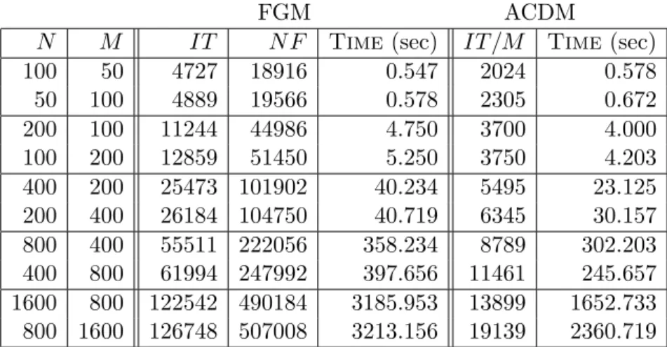
FGM

ACDM

N

M

IT

N F

Time

(sec)

IT /M

Time

(sec)

100

50

4727

18916

0

.

547

2024

0

.

578

50

100

4889

19566

0

.

578

2305

0

.

672

200

100

11244

44986

4

.

750

3700

4

.

000

100

200

12859

51450

5

.

250

3750

4

.

203

400

200

25473 101902

40

.

234

5495

23

.

125

200

400

26184 104750

40

.

719

6345

30

.

157

800

400

55511 222056

358

.

234

8789

302

.

203

400

800

61994 247992

397

.

656

11461

245

.

657

1600

800

122542 490184

3185

.

953

13899

1652

.

733

800 1600

126748 507008

3213

.

156

19139

2360

.

719

Table 1. Performance of FGM and ACDM on problem (4.1).

In this table, first two columns display the dimensions of problem (4.1). In all our

tests, the matrix

A

is dense. Therefore, for the largest problem we have more than one

million nonzero coefficients. Columns

IT

and

N F

show the number of iterations and

number of function evaluation of FGM. Column

IT /M

shows the number of blocks of

M

iterations in method ACDM. Finally, the column

Time

displays the total computational

time in seconds.

For us, the main characteristics of complexity of the problem for numerical scheme

is the total computational time. As we can see, ACDM always outperforms FGM. Its

domination is less impressive with respect to the theoretical prediction. However, this

can be explained by the ability of method (4.2) to use much smaller estimate of the

constant

L

(

f

µ

) than the worst-case theoretical value.

To conclude, we can see that potentially, ACDM is a promising computational scheme,

which has good chances to outperform FGM on many important real-life problems. At

this moment, as compared with FGM, ACDM has four main drawbacks:

•

absence of version with separable constraints;

•

impossibility to adjust the worst-case estimates for

L

i

(

f

) during the minimization

process;

•

absence of a reliable stopping criterion;

•

impossibility to generate good primal-dual solutions.

References

[1] Z. Allen-Zhu, Z. Qu, P. Richt´

arik, and Y. Yuan. Even faster accelerated coordinate

descent using non-uniform sampling. arXiv:1512.09103v2 [math.OC] 13 Jan 2016.

[2] Y.T. Lee and A. Sidford. Efficient accelerated coordinate descent methods and

fastest algorithms for solving linear systems. arXiv: 1305.1922v1, 8 May, 2013.

[3] Yu. Nesterov. A method for unconstrained convex minimization problem with the

rate of convergence

O

(

_k12

)

.

Doklady AN SSSR

(translated as Soviet Math. Docl.),

1983, v.269, No. 3, 543-547

[4] P. Richtarik and M. Taka˜c. Parallel coordinate descent methods for big data

opti-mization.

Mathematical Programming

, 1-51 (2012)

[5] P. Richtarik and M. Taka˜c. Distributed coordinate descent method for learning with

big data. arXiv: 1310.2059 (2012)

[6] Yu. Nesterov. Smooth minimization of non-smooth functions,

Mathematical

Pro-gramming

(A),

103

(1), 127-152 (2005).

[7] Yu.Nesterov. Efficiency of coordinate-descent methods on huge-scale optimization

problems.

SIOPT

,

22

(2), 341-362 (2012).

[8] Yu. Nesterov. Introductory lectures on Convex Optimization. The basic course.

Kluwer

, Boston (2004).

Recent titles

CORE Discussion Papers

2015/24 Wing Man Wynne LAM. Switching costs in two-sided markets.

2015/25 Philippe DE DONDER, Marie-Louise LEROUX. The political choice of social long term care transfers when family gives time and money.

2015/26 Pierre PESTIEAU and Gregory PONTHIERE. Long-term care and births timing.

2015/27 Pierre PESTIEAU and Gregory PONTHIERE. Longevitiy variations and the welfare State. 2015/28 Mattéo GODIN and Jean HINDRIKS. A review of critical issues on tax design and tax

administration in a global economy and developing countries

2015/29 Michel MOUCHART, Guillaume WUNSCH and Federica RUSSO. The issue of control in multivariate systems, A contribution of structural modelling.

2015/30 Jean J. GABSZEWICZ, Marco A. MARINI and Ornella TAROLA. Alliance formation in a vertically differentiated market.

2015/31 Jens Leth HOUGAARD, Juan D. MORENO-TERNERO, Mich TVEDE and Lars Peter ØSTERDAL. Sharing the proceeds from a hierarchical venture.

2015/32 Arnaud DUFAYS and Jeroen V.K. ROMBOUTS. Spare change-point time series models. 2015/33 Wing Man Wynne LAM. Status in organizations.

2015/34 Wing Man Wynne LAM. Competiton in the market for flexible resources : an application to cloud computing.

2015/35 Yurii NESTEROV and Vladimir SHIKHMAN. Computation of Fisher-Gale equilibrium by auction.

2015/36 Maurice QUEYRANNE and Laurence A. WOLSEY. Thight MIP formulations for bounded up/down tiems and interval-dependent start-ups.

2015/37 Paul BELLEFLAMME and Dimitri PAOLINI. Strategic promotion and release decisions for cultural goods.

2015/38 Nguyen Thang DAO and Julio DAVILA. Gender inequality, technologial progress, and the demographic transition.

2015/39 Thomas DEMUYNCK, Bram DE ROCK and Victor GINSBURGH. The transfer paradox in welfare space.

2015/40 Pierre DEHEZ. On Harsanyi dividends and asymmetric values.

2015/41 Laurence A. WOLSEY. Uncapacitated lot-sizing with stock upper bounds, stock fixed costs, stock overloads and backlogging: A tight formulation.

2015/42 Paul BELLEFLAMME. Monopoly price discrimination and privacy: the hidden cost of hiding. 2015/43 Pierre PESTIEAU and Gregory PONTHIERE. Optimal fertility under age-dependent labor

productivity.

2015/44 Jacques DREZE. Subjective expected utility with state-dependent but action/observation-independent preferences

2015/45 Joniada MILLA, Ernesto SAN MARTÍN and Sébastien VAN BELLEGEM. Higher education value added using multiple outcomes.

2015/46 Helmuth CREMER, Pierre PESTIEAU and Kerstin ROEDER. Social long-term care insurance with two-sided altruism.

2015/47 Per J. AGRELL and Humberto BREA-SOLÍS. Stationarity of heterogeneity in production technology using latent class modelling.

2015/48 Mattéo GODIN et Jean HINDRIKS. Disparités et convergence économiques : Ensemble mais différents.

Recent titles

CORE Discussion Papers

–

continued

2015/50 Benoît DECERF. A new index combining the absolute and relative aspects of income poverty: Theory and application.

2015/51 Pierre COPÉE, Axel GAUTIER and Mélanie LEFÈVRE. Promoting competition at the digital age with an application to Belgium.

2015/52 Mathieu LEFEBVRE, Sergio PERELMAN and Pierre PESTIEAU. Productivity and performance in the public sector.

2015/53 Oswaldo GRESSANI. Endogeneous quantal response equilibrium for normal form games. 2015/54 Wouter VERGOTE. One-to-one matching problems with location restrictions.

2015/55 Marie-Louise LEROUX, Dario MALDONADO and Pierre PESTIEAU. Compliance, informality and contributive pensions.

2015/56 Michel MOUCHART and Renzo ORSI. Building a structural model : Parameterization and structurality.

2016/01 Luc BAUWENS, Manuela BRAIONE, Giuseppe STORTI. A dynamic component model for forecasting high-dimensional realized covariance matrices.

2016/02 Manuela BRAIONE. A time-varying long run HEAVY model.

2016/03 Yurii NESTEROV and Sebastian STICH. Efficiency of accelerated coordinate descent method on structured optimization problems.

Books

W. GAERTNER and E. SCHOKKAERT (2012), Empirical Social Choice. Cambridge University Press. L. BAUWENS, Ch. HAFNER and S. LAURENT (2012), Handbook of Volatility Models and their

Applications. Wiley.

J-C. PRAGER and J. THISSE (2012), Economic Geography and the Unequal Development of Regions. Routledge.

M. FLEURBAEY and F. MANIQUET (2012), Equality of Opportunity: The Economics of Responsibility.

World Scientific.

J. HINDRIKS (2012), Gestion publique. De Boeck.

M. FUJITA and J.F. THISSE (2013), Economics of Agglomeration: Cities, Industrial Location, and Globalization. (2nd_{edition). Cambridge University Press.}

J. HINDRIKS and G.D. MYLES (2013). Intermediate Public Economics.(2nd_{edition). MIT Press.}

J. HINDRIKS, G.D. MYLES and N. HASHIMZADE (2013). Solutions Manual to Accompany Intermediate

Public Economics. (2nd_{edition). MIT Press.}

J. HINDRIKS (2015). Quel avenir pour nos pensions? Les grands défis de la réforme des pensions. De Boeck.

P. BELLEFLAMME and M. PEITZ (2015). Industrial Organization: Markets and Strategies (2nd_edition). Cambridge University Press.

CORE Lecture Series R. AMIR (2002), Supermodularity and Complementarity in Economics. R. WEISMANTEL (2006), Lectures on Mixed Nonlinear Programming. A. SHAPIRO (2010), Stochastic Programming: Modeling and Theory.