DOI: 10.1002/jae.2742
R E S E A R C H A R T I C L E
Two are better than one: Volatility forecasting using
multiplicative component GARCH-MIDAS models
Christian Conrad
Onno Kleen
Department of Economics, Heidelberg University, Heidelberg, Germany Correspondence
Onno Kleen, Department of Economics, Heidelberg University, Bergheimer Strasse 58, 69115 Heidelberg, Germany.
Email: [email protected]
Summary
We examine the properties and forecast performance of multiplicative volatility specifications that belong to the class of generalized autoregressive conditional heteroskedasticity–mixed-data sampling (GARCH-MIDAS) models suggested in Engle, Ghysels, and Sohn (Review of Economics and Statistics, 2013,95, 776–797). In those models volatility is decomposed into a short-term GARCH component and a long-term component that is driven by an explanatory variable. We derive the kurtosis of returns, the autocorrelation function of squared returns, and theR2of a Mincer–Zarnowitz regression and evaluate the QMLE and forecast performance of these models in a Monte Carlo simulation. For S&P 500 data, we compare the forecast performance of GARCH-MIDAS models with a wide range of competitor models such as HAR (heterogeneous autoregression), real-ized GARCH, HEAVY (high-frequency-based volatility) and Markov-switching GARCH. Our results show that the GARCH-MIDAS based on housing starts as an explanatory variable significantly outperforms all competitor models at forecast horizons of 2 and 3 months ahead.
1
I N T RO D U CT I O N
The idea of modeling volatility as consisting of multiple components has a long tradition in financial econometrics (see, e.g., Ding & Granger, 1996; Engle & Lee, 1999). Early models typically featured additive volatility components and did not allow for explanatory variables in the conditional variance. More recently, the focus has shifted to multiplicative component models (see, e.g., Amado & Teräsvirta, 2013, 2017; Engle, Ghysels, & Sohn, 2013; Engle & Rangel, 2008; Han & Kristensen, 2015). In particular, the class of generalized autoregressive conditional heteroskedasticity–mixed-data sampling (GARCH-MIDAS) models proposed in Engle et al. (2013) has been proven to be useful for analyzing the link between financial volatility and the macroeconomic environment (see Asgharian, Hou, & Javed, 2013; Conrad & Loch, 2015; Dorion, 2016). In GARCH-MIDAS, a unit-variance GARCH component fluctuates around a time-varying long-term component that is a function of (macroeconomic or financial) explanatory variables. By allowing for a mixed-frequency setting, this approach bridges the gap between daily stock returns and low-frequency (e.g., monthly, quarterly) explana-tory variables. For further applications of GARCH-MIDAS-type models see, for example, Conrad, Loch, and Rittler (2014), Opschoor, van Dijk, and van der Wel (2014), Dominicy and Vander Elst (2015), Lindblad (2017), Amendola, Candila, and Scognamillo (2017), Pan, Wang, Wu, and Yin (2017), Conrad, Custovic, and Ghysels (2018), and Borup and Jakobsen (2019). For a recent survey on multiplicative component models see Amado, Silvennoinen, and Teräsvirta (2019). Throughout this paper, the GARCH-MIDAS model will be our leading example for a multiplicative component GARCH (M-GARCH) model. However, we will also discuss how the class of M-GARCH models nests other specifications such as the Markov-switching GARCH (MS-GARCH) of Haas, Mittnik, and Paolella (2004), the spline-GARCH of Engle and Rangel (2008), and the multiplicative time-varying GARCH (MTV-GARCH) of Amado and Teräsvirta (2008).
This is an open access article under the terms of the Creative Commons Attribution-NonCommercial License, which permits use, distribution and reproduction in any medium, provided the original work is properly cited and is not used for commercial purposes.
© 2019 The Authors. Journal of Applied Econometrics published by John Wiley & Sons Ltd
Our contribution to this recent strand of literature is twofold. In the first part of this paper, we analyze several statistical properties of the GARCH-MIDAS model that have not received much attention so far. In the second part of the paper, we compare the out-of-sample (OOS) forecast performance of GARCH-MIDAS with the performance of various competitor models such as the heterogeneous autoregression (HAR) of Corsi (2009), the realized GARCH of Hansen, Huang, and Shek (2012), the high-frequency-based volatility (HEAVY) of Shephard and Sheppard (2010), and the MS-GARCH.
Our main theoretical findings can be summarized as follows. In the GARCH-MIDAS model, the kurtosis of the returns is always bigger than the kurtosis of the returns in the nested GJR-GARCH (see Glosten, Jagannathan, & Runkle, 1993) com-ponent. If the long-term component is sufficiently persistent, the autocorrelation function (ACF) of the squared returns as well as the ACF of the conditional variances is more persistent than the corresponding ACFs in the nested GJR-GARCH. Both findings suggest a multiplicative component structure in the volatility of stock returns as a potential explanation for the common failure of simple one-component GARCH models to adequately capture the stylized facts of returns and realized variances. It should also be noted that our results are remarkably similar to findings in Han (2015) on GARCH-X models, even though Han considers models with an additive explanatory variable in the conditional variance and focuses on the asymptotic limit of the sample kurtosis and the sample ACF. Further, we derive an upper bound for the
popula-tionR2in thek-step-ahead Mincer and Zarnowitz (1969) regression (henceforth MZ regression) of the squared return
on the volatility forecast. We show that the populationR2decreases monotonically in the forecast horizon but increases
monotonically in the variability of the long-term component. The latter feature leads to the unpleasant property that the goodness-of-fit is particularly high in situations in which the squared error loss is also high. Clearly, this finding
ques-tions the usefulness of the MZR2for comparing forecast accuracy across volatility regimes. In this context, we derive an
explicit expression for the one-step-aheadR2of the GARCH-MIDAS specification and obtain the results from Andersen
and Bollerslev (1998) for the simple GARCH(1,1)as a special case.
Empirically, we first evaluate the quasi-maximum likelihood estimator (QMLE) of GARCH-MIDAS models by means of a Monte Carlo simulation. We show that the QMLE is unbiased and that the asymptotic standard errors based on Wang and Ghysels (2015) are valid in the presence of exogenous explanatory variables. Further, we show that measurement error in the explanatory variable or a misspecification of the lag structure has only minor effects. We also confirm our
theoretical result that theR2 of a MZ regression is highest in regimes with high volatility, although in those regimes
forecast performance is the worst. Following the arguments put forth in Patton and Sheppard (2009) and Patton (2011), we use the QLIKE to evaluate the OOS forecast performance of the GARCH-MIDAS model against the MS-GARCH and the nested GARCH. We find that the correctly specified and, in most settings, even the misspecified GARCH-MIDAS models beat the competitor models.
Finally, we apply the GARCH-MIDAS model to a long time series of S&P 500 returns combined with data on US macroeconomic and financial conditions. We consider GARCH-MIDAS models with one or two explanatory variables and, for the OOS forecast evaluation, estimate all models on a rolling window using the appropriate real-time vintage data. Because macroeconomic time series are revised substantially after the first release, we avoid a “look-ahead-bias” by using real-time data. In the OOS forecast evaluation, we compare the GARCH-MIDAS with eight competitor mod-els: Among those competitor models are the realized GARCH, the HEAVY, the MS-GARCH, and HAR models with and without leverage. We evaluate all models jointly by constructing model confidence sets (MCS) as introduced in Hansen, Lunde, and Nason (2011). For forecast horizons of 2 weeks and 1 month, the MCS consists of the realized GARCH, the HAR, and GARCH-MIDAS models with the CBOE Volatility Index (VIX) (or the VIX combined with another explana-tory variable). That is, at these forecast horizons the GARCH-MIDAS is on a par with those models but beats the HEAVY as well as MS-GARCH models. At longer forecast horizons of 2 and 3 months ahead, only GARCH-MIDAS models are included in the MCS. At both horizons the GARCH-MIDAS based on housing starts achieves the lowest QLIKE. This find-ing is remarkable because our OOS period begins in 2010 and hence does not include the financial crisis and the collapse of the housing bubble.
To facilitate the replication of our results, we provide R packages for downloading real-time data from the ALFRED database of the Federal Reserve Bank of St. Louis (see Kleen, 2017), as well as for estimating GARCH-MIDAS models (see Kleen, 2018).1
Our paper is organized as follows: In Section 2, the M-GARCH model and our theoretical results are presented. In Section 3, we perform a simulation study and, in Section 4, we apply the GARCH-MIDAS model to S&P 500 return data. The conclusion follows in Section 5. All proofs are contained in Supporting Information Appendix A of the Online Appendix. Additional material can be found in Appendices B–H.
2
T H E M U LT I P L I C AT I V E CO M P O N E N T GA RC H M O D E L
In this section, the M-GARCH model is introduced and its theoretical properties are derived. In particular, we show that the M-GARCH model inherits certain time series properties that are in line with stylized facts typically observed for financial return data but cannot be captured by simple GARCH models.
2.1
Model specification
We denote daily log-returns byri,t, whereby the indext=1,…,Trefers to a certain period (e.g., a week or a month) and
the indexi=1,…,Itto days within that period. For simplicity, we model the returns asri,t= 𝜇+𝜀i,t.2The M-GARCH
model assumes that the scaled (demeaned) returns can be written as 𝜀i,t
√ 𝜏t
=√gi,tZi,t, (1)
where𝜏tis specified as a function of a (low-frequency) explanatory variableXt,gi,tfollows a GARCH equation, andZi,tis
an i.i.d. innovation process with mean zero and variance one. Leti,tdenote the information set up to dayiin periodt
and definet∶=It,t. If𝜏tdepends on lagged values ofXtonly, then
𝜎2
i,t∶=gi,t𝜏t (2)
is the conditional variance of the daily returns; that is,𝜎2
i,t =var(𝜀i,t|i−1,t). We refer togi,tas the short-term component
of volatility and to𝜏t as the long-term component of volatility. Whereasgi,t varies daily,𝜏t is constant across all days
within periodt and thus changes at the lower frequency only. The short-term component is intended to describe the
well-known day-to-day clustering of volatility and is assumed to follow a mean-reverting unit-variance GJR-GARCH(1,1) process: gi,t= (1−𝛼−𝛾∕2−𝛽) +(𝛼+𝛾𝟙{𝜀i−1,t<0} )𝜀2 i−1,t 𝜏t +𝛽gi−1,t. (3)
Remark1. We use the convention that 𝜀0,t = 𝜀It−1,t−1 and g0,t = gIt−1,t−1. Similarly, we can write the long-term
component as𝜏i,t =𝜏tfori= 1,…,nand𝜏0,t = 𝜏It−1,t−1 =𝜏t−1. That is, forIt > 1,𝜏tis piecewise constant. IfIt = 1,
then both components vary at the same frequency. In this case we can write𝜀1,t = 𝜀t,g1,t = gt,𝜀0,t = 𝜀1,t−1 = 𝜀t−1,
andg0,t=g1,t−1=gt−1. Thus we can drop the indexi.
A characteristic of the two-component M-GARCH model defined in Equation (1) is that the scaled returns,𝜀i,t∕√𝜏t,
are assumed to follow a GARCH process. Hence the forcing variable in Equation (3) is𝜀2
i−1,t∕𝜏t. This feature distinguishes
the two-component M-GARCH specification from standard GARCH models. In those models it is assumed that𝜏t = 1
and hence the returns themselves follow a GARCH process. Similarly, additive component GARCH models, such as
the model of Engle and Lee (1999), assume that 𝜏t = 1 and decompose gi,t into two or more GARCH components
(with forcing variable𝜀2
i−1,t). We make the following assumptions regarding the innovation processZi,tand the parameters
of the short-term component.
Assumption 1. LetZi,tbe i.i.d. withE[Zi,t] =0,E[Zi,t2] =1, and 1< 𝜅 <∞, where𝜅=E[Z4i,t].
Assumption 2. We assume that𝛼 >0,𝛼+𝛾 >0,𝛽 ≥ 0, and𝛼+𝛾∕2+𝛽 <1. Moreover, the parameters satisfy the condition(𝛼+𝛾∕2)2𝜅+2(𝛼+𝛾∕2)𝛽+𝛽2<1.
Assumptions 1 and 2 imply that𝜀i,t∕√𝜏t= √
gi,tZi,tis a covariance stationary GJR-GARCH(1,1) process. The first- and
second-order moments ofgi,tare given byE[gi,t] =1,
E[gi2,t] = 1− (𝛼+𝛾∕2+𝛽) 2
1− (𝛼+𝛾∕2)2𝜅−2(𝛼+𝛾∕2)𝛽−𝛽2, (4)
2It would be straightforward to allow for richer dynamics in the conditional mean. However, for daily return data a constant conditional mean is usually
and the fourth moment of√gi,tZi,tis finite. The role of the second component,𝜏t, is to describe smooth movements in the
conditional variance. In general, we specify𝜏tas a measurable, positive-valued function,f(·), of the present andK ≥ 1
lagged values of an explanatory variableXt:
𝜏t =𝑓(Xt,Xt−1,…,Xt−K). (5)
The appropriate choice of the explanatory variableXtand of the functionf(·)is up to the researcher and will depend on
the specific application at hand.3The explanatory variable can either vary at the daily frequency (i.e.,I
t =1) or at a lower
frequency (i.e.,It>1). Thus, the choice ofXtdefines the low frequencyt. In GARCH-MIDAS-type models𝜏tdepends on
lagged values ofXtonly. By explicitly allowing𝜏tto depend onXtin Equation (5), we ensure that our setting also covers
MS-GARCH models (see Section 2.2 for details). We make the following assumption about the explanatory variableXt
and the functionf(·):
Assumption 3. Letf(·) > 0 be a measurable function andXt be a strictly stationary and ergodic time series with
E[|Xt|q]<∞, whereqis sufficiently large to ensure thatE[𝜏t2]<∞.Xtis independent ofZi,t−jfor allt,iandj.
Note that Assumption 3 implies that𝜏tis strictly stationary (see Billingsley, 1995, p. 495), covariance stationary, and
independent of the ‘GARCH part’ (i.e.gi,t−𝑗Zi2,t−𝑗) of the model. In empirical applications the functionf(·) > 0 is often
chosen as being linear in the laggedXt:
𝜏t=m+𝜋1Xt−1+ … +𝜋KXt−K. (6)
The linear specification requiresm>0 and𝜋l ≥ 0, forl=1,…,K, and is feasible only ifXtis a nonnegative variable.
IfXtcan take positive as well as negative values, it is natural to opt for an exponential specification:
𝜏t=exp(m+𝜋1Xt−1+ … +𝜋KXt−K). (7)
The assumption thatXt is independent ofZi,t−jfor allt,i, andjmight appear to be rather strong. However, without
imposing any restrictions on the functional form off(·), it greatly simplifies the analysis when discussing the statistical
properties of M-GARCH models in Section 2.3. From an empirical perspective, we believe that it is reasonable to assume
that a low-frequency explanatory variableXt—such as monthly industrial production growth—is (close to being)
indepen-dent of the daily innovationsZi,t−j. For daily explanatory variables (e.g., measures of realized volatility) the independence
assumption might appear to be restrictive. However, even if there is a dependence between the innovation to the daily
returns and the daily explanatory variable, the dependence between𝜏tandZi,t−jis likely to be negligible. This is because
𝜏tis a rather smooth function that is obtained as a weighted average of many lags of the dailyXt. Indeed, in Section 3 and
Supporting Information Appendix D we illustrate in simulations that a mild violation of the independence assumption does not affect our main results.
It should also be noted that the same independence assumption has been previously made in related literature on M-GARCH models (see Han & Kristensen, 2015). Nevertheless, it clearly imposes a limitation that should be overcome in future work. Two examples in this direction are the estimation of GARCH-MIDAS models employing lagged values of realized variances (Wang & Ghysels, 2015) and testing for an omitted long-term component in one-component GARCH models (Conrad & Schienle, 2018).
Assumptions 1, 2, and 3 imply that the𝜀i,thave mean zero, are uncorrelated, and have an unconditional variance given
by var(𝜀i,t) =E[𝜏t]. Moreover, the unconditional variance of the squared returns is well defined: var(𝜀2i,t) =𝜅E[𝜏t2]E[g2 i,t] −
E[𝜏t]2. If the long-term component is constant and chosen as𝜏
t=𝜔∕(1−𝛼−𝛾∕2−𝛽), our model reduces to the GJR-GARCH
with intercept𝜔.
A measure that is often used to quantify the relative importance of the long-term component is the following variance ratio (see Engle et al., 2013):
VR=var(log(𝜏t))∕var(log(𝜏tgt)), (8)
wheregt=
∑It
i=1gi,t. The ratio measures how much of the total variation in the (log) conditional variance can be explained
by the variation in the (log) long-term component.
3While we focus on multiplicative GARCH models, Han and Park (2014) and Han (2015) analyze the properties of a GARCH-X specification with an
2.2
Nested and related specifications
We first discuss two models that are directly nested in the M-GARCH setting. The two models are the GARCH-MIDAS of Engle et al. (2013) and (a restricted version of) the MS-GARCH model of Haas et al. (2004). Closely related are the Spline-GARCH of Engle and Rangel (2008) and the MTV-GARCH of Amado and Teräsvirta (2008). For further models that have a multiplicative component structure see Amado et al. (2019).
2.2.1
GARCH-MIDAS
In the GARCH-MIDAS the long-term component is defined as in Equation (6) or (7), whereby the weights 𝜋l are
parsimoniously specified via a weighting scheme. The most common choice of long-term component is based on the exponential specification with𝜋l=𝜃·𝜑l(w1,w2). Here, the parameter𝜃determines the sign of the effect of the laggedXt
on the long-term component and the weights𝜑l(w1,w2) ≥ 0 are parametrized via the Beta weighting scheme
𝜑l(w1,w2) = [l∕(K+1)]w1−1· [1−l∕(K+1)]w2−1 K ∑ 𝑗=1 [𝑗∕(K+1)]w1−1· [1−𝑗∕(K+1)]w2−1 . (9)
By construction, the weights sum to one; that is, ∑Kl=1𝜑l(w1,w2) = 1. It directly follows that E[𝜏t+1|t] = 𝜏t+1.
Engle et al. (2013) use monthly industrial production growth and monthly inflation as explanatory variables, whereas Conrad and Loch (2015) employ quarterly macroeconomic variables such as gross domestic product (GDP) growth. For further applications of this model see Asgharian et al. (2013), Opschoor et al. (2014), and Dorion (2016). Wang and Ghysels (2015) consider the special case thatf(·)is linear,It = 1 andXt = ∑𝑗J=−10𝜀2t−𝑗. That is,Xtis the realized variance
based on the lastJdaily returns. Note that for this specificationXtandZtare dependent and hence Assumption 3 would
be violated.
2.2.2
MS-GARCH
In MS-GARCH the returns are given by𝜀t= ̃𝜎Xt,tZt, where{Xt}is a Markov chain with finite state spaceS= {1,2,…,s}
and transition matrixPwith typical elementpi,j = P(Xt = j|Xt−1 = i). A restricted version of the MS-GARCH model
of Haas et al. (2004) is nested in our setting withIt = 1. This is best illustrated in the case ofs = 2: We assume that
the conditional variances in the regimes differ in the intercepts but have the same ARCH and GARCH parameters; for example,̃𝜎2
k,t=𝜔k+𝛼𝜀2t−1+𝛽 ̃𝜎k,t2 −1,k∈S. Defining𝜏t= [(2−Xt)𝜔1+ (Xt−1)𝜔2]∕(1−𝛼−𝛽), we can rewrite the returns
as𝜀t = √
̃𝜎2 Xt,tZt =
√
gt𝜏tZt, wheregt = (1−𝛼−𝛽) + (𝛼Z2t−1+𝛽)gt−1. Thus the conditional variance has a multiplicative
structure. In the following, we will refer to this model as MS-GARCH with time-varying intercept (MS-GARCH-TVI). Stationarity conditions for MS-GARCH models can be found in Haas et al. (2004).
2.2.3
Spline-GARCH and multiplicative time-varying (MTV) GARCH
In both models it is assumed thatIt=1. The spline-GARCH model specifies the long-term component as a spline function
and chooses Xt = t. Similarly, in the MTV-GARCH f(·) is specified in terms of logistic transition functions and
Xt=t∕Tis the rescaled time. Thus in both models the long-term component is a deterministic function of time and hence
Assumption 3 is violated.
2.3
Properties of the M-GARCH
In the following, we derive properties of M-GARCH models for which Assumptions 1, 2, and 3 are satisfied.
2.3.1
Kurtosis and autocorrelation function
Financial returns are often found to be leptokurtic. Hence a desirable feature of a volatility model is that it generates returns with a kurtosis that is similar to the one empirically observed for financial returns. Under Assumptions 1, 2, and 3, the kurtosis of the returns defined in Equation (1) is given by
MG= E [ 𝜀4 i,t ] ( E [ 𝜀2 i,t ])2 = E [ 𝜎4 i,t ] ( E [ 𝜎2 i,t ])2𝜅 > 𝜅.
Thus the kurtosis of the M-GARCH process is larger than the kurtosis of the innovationZi,t. This is a well-known feature
of GARCH-type processes. The following proposition relates the kurtosisMGof the M-GARCH to the kurtosisGAof
the nested GARCH(1,1).
Proposition 1. Under Assumptions 1-3, the kurtosisMGof an M-GARCH process is given by
MG= E [ 𝜏2 t ] E[𝜏t]2 · GA≥ GA, whereGA=𝜅·E[g2
i,t]is the kurtosis of the nested GARCH process and where the equality holds if and only if𝜏tis constant.
Hence, for nonconstant𝜏t, the kurtosisMGis the product ofGAand the ratioE[𝜏t2]∕E[𝜏t]2>1. When𝜏t=𝜔∕(1−𝛼−
𝛾∕2−𝛽)is constant, Proposition 1 nests the kurtosis of the GJR-GARCH model. Thus, for volatile long-term components
the kurtosis of an M-GARCH process can be much larger than the kurtosis of the nested GARCH model.4Specifically,
Proposition 1 holds for the GARCH-MIDAS and for the MS-GARCH-TVI defined in Section 2.2.
The empirical ACFs of volatility proxies such as squared returns or realized variances are known to be very persistent (see, e.g., Andersen, Bollerslev, Diebold, & Labys, 2003; Ding, Granger, & Engle, 1993). In particular, squared returns are
often found to decay more slowly than the exponentially decaying ACF implied by the simple GARCH(1,1)model. In the
literature on GARCH models, this is usually interpreted as either evidence for long memory (see, e.g., Baillie, Bollerslev, & Mikkelsen, 1996), structural breaks (see, e.g., Hillebrand, 2005), or an omitted persistent covariate (see Han & Park, 2014) in the conditional variance.
The following propositions show that the theoretical ACFs of the M-GARCH process have a much slower decay than the ACF of the nested GARCH component if the long-term component is sufficiently persistent. Hence the multiplicative structure provides an alternative explanation for the empirical observation of highly persistent ACFs of squared returns or realized variances. For Propositions 2 and 3, we consider the case that both components are varying at the same frequency; that is, the length of the periodtis one day(It=1).
Proposition 2. If It=1and Assumptions 1-3 are satisfied, the ACF,𝜌MGk (𝜀2), of the squared returns from an M-GARCH process is given by 𝜌MG k (𝜀 2) =corr(𝜀2 t, 𝜀 2 t−k) =𝜌𝜏k var(𝜏t) var(𝜀2 t) +𝜌GAk var(gtZ 2 t) var(𝜀2 t) ( 𝜌𝜏 kvar(𝜏t) +E[𝜏t] 2) (10)
with𝜌𝜏k=corr(𝜏t, 𝜏t−k)and
𝜌GA k =corr(gtZ 2 t,gt−kZ2t−k) = (𝛼+𝛾∕2+𝛽)k−1 (𝛼+𝛾∕2)[1− (𝛼+𝛾∕2)𝛽−𝛽2] 1−2(𝛼+𝛾∕2)𝛽−𝛽2 being the ACF of the GJR-GARCH component.5
Proposition 2 shows that the ACF of the squared returns is given by the sum of two terms: the first term corresponds to
the ACF of the long-term component𝜌𝜏
ktimes a constant, whereas the second term equals the exponentially decaying ACF
of the nested GARCH model𝜌GA
k times a term that depends again on𝜌𝜏k. Hence, if𝜏tis sufficiently persistent,𝜌 MG k (𝜀 2)will essentially behave as𝜌𝜏 kforklarge. 6For𝜏
tbeing constant, the first term in Equation (10) is equal to zero and the second
4Han (2015) obtains a similar result for the sample kurtosis of the returns from a GARCH-X model with a covariate that can either be stationary or
nonstationary.
5Note that𝜌GA
k reduces to the ACF of a (symmetric) GARCH(1,1)when𝛾=0(see Karanasos, 1999).
6Again, Han (2015) also obtains a bicomponent structure for the sample ACF of the squared returns from a GARCH-X model with a fractionally
integrated covariate. Similarly, Han and Kristensen (2015) show that the empirical ACF in a multiplicative model can display long-memory-type behavior.
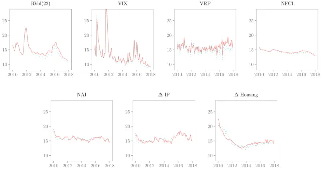
FIGURE 1 Autocorrelation function of the volatility process in a GARCH-MIDAS model. We depict the ACF of the volatility process in a GARCH-MIDAS model (red, dashed) and its components: the first (green, solid) and second term (blue, dot-dashed) in
Equation (11). The long-term component is defined as in
Equations (7) and (9) withm= −0.1,𝜃=0.3,w1=1,w2=5, and
K=264. The explanatory variable is given by
Xt=𝜙Xt−1+𝜉t, 𝜉t
i.i.d. ∼ (0, 𝜎2
𝜉), where𝜙=0.98 and𝜎𝜉2=0.352.
The GARCH(1,1)parameters are𝛼=0.06,𝛽=0.91, and𝛾=0.
Moreover, we set𝜅=3. Bars in light gray display the empirical
autocorrelation of S&P 500 daily realized variances between 2000:M1 and 2018:M4 as measured by Hansen and Lunde (2014). For details see Section 4 [Colour figure can be viewed at wileyonlinelibrary.com] term reduces to the ACF of an asymmetric GARCH(1,1). Also, note that the ratio var(𝜏t)∕var(𝜀2t)is closely related to the variance ratio defined in Equation (8) and measures how much of the variation in the squared returns can be attributed to the variation in the long-term component; that is, it measures the importance of the long-term component.
Haas et al. (2004, p. 503) make a similar observation for the MS-GARCH-TVI model that we discussed in Section 2.2.
For this model, they show that the autocorrelations of the squared returns decay at a rate of max{𝛼+𝛽, 𝜛}, where𝜛=
p1,1+p2,2−1 is the degree of persistence due to the Markov effects.7If𝜛is close to one—that is, if the long-term component
is very persistent—the decay rate of this component dominates the decay of the autocorrelation function.
A standard misspecification test for GARCH models is the Ljung–Box statistic applied to the squared deGARCHed residuals,𝜀2
t∕gt. The result in Proposition 2 may explain why in empirical applications the null hypothesis of this test is
often rejected. In the multiplicative model, the ACF of the squared deGARCHed residuals is given by𝜌𝜏
k·var(𝜏t)∕(𝜅E[𝜏 2 t] −
E[𝜏t]2), which follows the rate of decay of the long-term component and hence is still persistent. Using similar arguments
to those in the proof of Proposition 2, we can derive the ACF of𝜎2
t.
Proposition 3. If It=1and Assumptions 1-3 are satisfied, the ACF,𝜌MGk (𝜎2), of𝜎t2is given by
𝜌MG k (𝜎 2) =corr(𝜎2 t, 𝜎t2−k ) =𝜌𝜏kvar(𝜏t) var(𝜎2 t) +𝜌gkvar(gt) var(𝜎2 t) ( 𝜌𝜏 kvar(𝜏t) +E[𝜏t] 2) (11)
with𝜌𝜏kas before and𝜌gk=corr(gt,gt−k) = (𝛼+𝛾∕2+𝛽)kbeing the ACF of the gtcomponent.
Again, Assumption 3 holds for the GARCH-MIDAS and the MS-GARCH-TVI.
The implications of Proposition 3 are depicted in Figure 1. The bars in light gray display the empirical ACF of the
daily S&P 500 realized variances for the 2000:M1 to 2018:M4 period.8 The autocorrelations were estimated using the
instrumental variables estimator suggested in Hansen and Lunde (2014). We employ their preferred specification, a two-stage least squares estimator in which lagged realized variances of order 4–10 are used as instrumental variables (see Hansen & Lunde, 2014, p. 82). By choosing appropriate parameter values for a GARCH-MIDAS process, we obtain
an ACF of𝜎2
t (dashed red line), which behaves very similar to the empirical ACF of the realized volatilities. The figure
shows that the second term—that is, the ACF ofgt(dot-dashed blue line)—determines the decay behavior of𝜌k(𝜎2)MG
whenkis small, whereas the first term—that is, the ACF of𝜏t(solid green line)—dominates whenkis large. Finally, it is
important to note that although our results on the kurtosis and the ACFs are presented for a GJR-GARCH(1,1)short-term
component, they directly extend to a covariance stationary GJR-GARCH(p,q) component.
2.3.2
Forecast evaluation with MZ regression
In empirical applications, the coefficient of determination from an MZ regression is often used as a measure of forecast accuracy. In this section, we will argue against using this measure when comparing forecast performance across volatility regimes. We now exclusively focus on the case of a GARCH-MIDAS. We assume that forecasts are produced on the last
dayIt of period tand denote thek-step-ahead volatility forecast byhk,t+1|t withk ≤ It+1. The optimal forecast from
7Haas et al. (2004) consider a symmetric GARCH. Hence the persistence in the GARCH component is𝛼+𝛽.
the GARCH-MIDAS ishk,t+1|t =E [ 𝜎2 k,t+1|t ] =𝜏t+1gk,t+1|t, where gk,t+1|t =E [ gk,t+1|t ] =1+ (𝛼+𝛾∕2+𝛽)k−1(g 1,t+1|t−
1). When evaluating the volatility forecast, one has to deal with the problem that the true conditional variance,𝜎2
k,t+1,
is unobservable. Patton (2011) discusses the situation in which the forecast evaluation is based on some conditionally unbiased volatility proxŷ𝜎2
k,t+1instead. He defines a loss functionL (
𝜎2
k,t+1,hk,t+1|t )
asrobustif the expected loss ranking
of two competing forecasts is preserved when replacing𝜎2
k,t+1by ̂𝜎 2
k,t+1. In the MZ regression𝜎 2
k,t+1is often replaced by the
conditionally unbiased but noisy proxŷ𝜎2
k,t+1=𝜀 2 k,t+1.
9
The MZ regression for evaluating thek-step-ahead volatility forecast is given by
𝜀2
k,t+1=𝛿0+𝛿1hk,t+1|t+𝜂k,t+1. (12)
We denote the respective coefficient of determination byR2k. As shown in Hansen and Lunde (2006), the ranking of
com-peting one-step-ahead volatility forecasts based on theR2
1of the MZ regression is robust to using the proxy𝜀
2
1,t+1instead
of the latent conditional variance𝜎2
1,t+1as the dependent variable. Forhk,t+1|t =𝜏t+1gk,t+1|t, the population parameters of
the MZ regression are given by𝛿0=0 and𝛿1=1 and hence the populationR2kcan be written as
R2k =1− var(𝜂k,t+1) var ( 𝜀2 k,t+1 ) =1− E [ SE ( 𝜀2 k,t+1,hk,t+1|t )] var ( 𝜀2 k,t ) , (13)
where we use that the variance of𝜂k,t+1equals the expected squared error (SE) loss of the forecast evaluated against𝜀2
k,t+1; that is,E [ SE ( 𝜀2 k,t+1,hk,t+1|t )] =E [( 𝜀2 k,t+1−hk,t+1|t )2] . Using thatE [ 𝜀2 k,t+1|k−1,t+1 ] =𝜎2 k,t+1, it follows that E [ SE ( 𝜀2 k,t+1,hk,t+1|t )] =E [ SE ( 𝜎2 k,t+1,hk,t+1|t )] + (𝜅−1)E [ 𝜎4 k,t+1 ] . (14)
That is, the expected SE based on the noisy proxy equals the expected SE based on the latent volatility plus a term that
depends on the fourth moment,𝜅, ofZi,tand the expected value of the squared conditional variance. Hence using a noisy
proxy for forecast evaluation can lead to a substantially higher expected SE than the expected SE based on the latent volatility. Patton, (2011, p. 248) basically makes the same point by arguing that “although the ranking obtained from a
robust loss function will be invariant to noise in the proxy, the actuallevelof expected loss obtained using a proxy will be
larger than that which would be obtained when using the true conditional variance.”
Using the insight from Equation (14) that the expected SE loss based on the noisy proxy is at least(𝜅−1)E
[ 𝜎4
k,t ]
, we obtain the following bound:
R2k ≤1− (𝜅−1)E [ 𝜎4 k,t ] 𝜅E [ 𝜎4 k,t ] − ( E [ 𝜎2 k,t ])2 = 1− ( E [ 𝜎2 k,t ])2 ∕E [ 𝜎4 k,t ] 𝜅− ( E [ 𝜎2 k,t ])2 ∕E [ 𝜎4 k,t ] < 𝜅1. (15)
The upper bound for R2
k given by Equation (15) nicely illustrates that a low R
2
k is not necessarily evidence for
model misspecification but can simply be due to using a noisy volatility proxy. This point has been made before by
Andersen and Bollerslev (1998), but for the special case of a one-step-ahead forecast from a GARCH(1,1).10Note that the
result in Equation (15) does not depend on the two-component structure of the model but is true for any conditionally heteroskedastic process.
Next, we derive an explicit expression for the MZR2
kof the GARCH-MIDAS model.
9To illustrate the severeness of the noise, consider an example withZ
k,t+1 ∼(0,1). Then𝜀2k,t+1will either over- or underestimate the true𝜎
2
k,t+1by
more than 50% with a probability of about 74%.
Proposition 4. If𝜀2
k,t+1 follows a GARCH-MIDAS process, Assumptions 1-3 are satisfied, and hk,t+1|t = 𝜏t+1gk,t+1|t, then the population R2kof the MZ regression is given by
R2k= var(hk,t+1|t) var ( 𝜀2 k,t+1 ) = E [ g2 k,t+1|t ] E[𝜏2 t+1 ] −E[𝜏t+1]2 E [ g2 k,t+1 ] E[𝜏2 t+1 ] 𝜅−E[𝜏t+1]2 (16) withE [ g2 k,t+1 ] as in Equation (4) and E [ g2k,t+1|t ] =1+ (𝛼+𝛾∕2+𝛽)2(k−1)(E[g21,t+1]−1). (17) We obtain the following two properties:
1. R2
k decreases monotonically with increasing forecast horizon k and, in the limit, converges
11 to R2 ∞ = var(𝜏t+1)∕var ( 𝜀2 k,t+1 ) . 2. R2 kincreases monotonically inE [ 𝜏2 t+1 ] .
The first property rests on the insight that the forecast of the GARCH component converges to one (ask → ∞) and
hence the MZ regression reduces to a regression of𝜀2
k,t+1on a constant and𝜏t+1. ThusR 2
∞can be interpreted as the fraction
of the total variation in daily returns that can be attributed to the variation in the long-term component. Note thatR2
∞
corresponds to the weight that is attached to the ACF of𝜏tin the first term in Equation (10).
Second, the result thatR2
k increases when𝜏t+1gets more volatile implies that for the very same model theR
2
k will be
higher in high-volatility regimes (i.e., when the squared error loss is high) than in low-volatility regimes (i.e., when the
squared error loss is low). This can be misleading when calculatingR2
kfor different regimes. The intuition is best illustrated
when looking at one-step-ahead forecasts. Equations (13) and (14) imply
R21=1− E [ SE ( 𝜀2 1,t+1,h1,t+1|t )] var ( 𝜀2 1,t+1 ) =1− (𝜅−1)E [ g2 1,t+1 ] E[𝜏2 t+1 ] E [ g2 1,t+1 ] E[𝜏2 t+1 ] 𝜅−E[𝜏t+1]2 . (18)
WhenE[𝜏t2+1]is increasing, the unconditional variance of returns rises at a faster rate than the expected squared error
and hence the MZR2
1is increasing. We can expressR21directly as a function of the model parameters:
Lemma 1. If𝜀2
k,t+1follows a GARCH-MIDAS process, Assumptions 1-3 are satisfied, and h1,t+1|t = 𝜏t+1g1,t+1, then the population R2
1of the MZ regression is given by R21= [1− (𝛼+𝛾∕2+𝛽) 2]E[𝜏2 t+1 ] − [1− (𝛼+𝛾∕2)2𝜅−2(𝛼+𝛾∕2)𝛽−𝛽2]E[𝜏 t+1]2 [1− (𝛼+𝛾∕2+𝛽)2]E[𝜏2 𝜏+1 ] 𝜅− [1− (𝛼+𝛾∕2)2𝜅−2(𝛼+𝛾∕2)𝛽−𝛽2]E[𝜏 t+1]2 . (19)
For𝜏t+1being constant and𝛾 =0, Equation (19) is reduced to the expression in Andersen and Bollerslev (1998, p. 892)
for the symmetric GARCH(1,1); that is,R2 1=𝛼
2∕(1−2𝛼𝛽−𝛽2).
The effect of an increase in E[𝜏t2+1]on E [ SE ( 𝜀2 1,t+1,h1,t+1|t )] , var ( 𝜀2 1,t+1 )
andR21 is illustrated in Figure 2. We set
E[𝜏t+1] = 1,𝛼 = 0.05, 𝛽 = 0.92, 𝛾 = 0, and𝜅 = 3. As expected, the left-hand panel shows that the expected squared
error increases when we move from a low-volatility regime (sayE[𝜏t2+1] = 2) to a high-volatility regime (sayE[𝜏t2+1]=
5). However, it also shows that the variance of the returns is increasing even faster (as evident from the larger slope
coefficient). The right-hand panel of Figure 2 shows that this translates into an increase ofR2
1. That is, although the
expected squared error increases, the “forecast accuracy” as measured byR2
1increases as well. In this regard, theR
2of
an MZ regression should be interpreted as a measure ofrelativeforecast accuracy; that is, forecast accuracy is measured
11Although by assumptionk ≤ I
tin our setting, we can think of, for example, a semiannual period and daily volatility forecasts. In this casekcan be
at most 132 (=6·22). For such a largekand under reasonable assumptions on the GARCH parameters, we haveE[g2
132,t+1|t
]
FIGURE 2 E[SE(𝜀2 1,t+1,h1,t+1|t )] , var(𝜀2 1,t+1 ) , and MZR2 1as a function of E[𝜏2 t+1 ]
. The left-hand panel shows E[SE(𝜀2
1,t+1,h1,t+1|t )]
(red, solid) and
var(𝜀2
1,t+1
)
(blue, dashed) as a function
ofE[𝜏2
t+1
]
(see Equation (18)). The right-hand panel depicts the corresponding population Mincer-ZarnowitzR2 1as a function of E[𝜏2 t+1 ] . We setE[𝜏t+1] =1, 𝛼=0.05, 𝛽=0.92, 𝛾=0, and𝜅=3
[Colour figure can be viewed at wileyonlinelibrary.com]
relative to the unconditional variance of the process. In contrast, the squared error loss is a measure ofabsoluteforecast
accuracy. Note that for rather moderate values ofE[𝜏t2+1]the coefficient of determination is already close to its upper
bound of 1/3.
Although the previous results are derived under the assumption that squared daily returns are used as the volatility proxy, it is true that the main insights still hold when using a better volatility proxy. For example, consider the hypothetical
case of observing𝜎2
k,t+1ex post. Then, fork →∞, we obtainR
2 ∞ =var(𝜏t+1)∕var ( 𝜎2 k,t+1 ) < 1. HenceR2
∞would still vary
across volatility regimes and increase in the variance of the long-term component. In the simulation in Section 3, we will
consider the case in which the realized variance is used as a proxy for𝜎2
k,t+1.
Finally, we consider cumulative volatility forecasts. The MZ regression for evaluating the cumulativek-day-ahead
volatility forecast is given by
̃
RV1∶k,t+1= ̃𝛿0+ ̃𝛿1h1∶k,t+1|t+𝜂1∶k,t+1,
where the latent variance is proxied by the realized varianceRṼ1∶k,t+1 =
∑k
i=1𝜀2i,t+1(purely based on daily return data)
andh1∶k,t+1|t=
∑k
𝑗=1h𝑗,t+1|t. The correspondingR21∶kis given by
R21∶k = var(h1∶k,t+1|t) var(RṼ1∶k,t+1) = E[𝜏2 t+1 ] E ⎡ ⎢ ⎢ ⎣ ( k ∑ i=1 gi,t+1|t )2⎤ ⎥ ⎥ ⎦ −k2E[𝜏 t+1]2 E[𝜏2 t+1 ] E ⎡ ⎢ ⎢ ⎣ ( k ∑ i=1 gi,tZ2 i,t )2⎤ ⎥ ⎥ ⎦ −k2E[𝜏 t+1]2 . (20)
As before, one can show thatR2
1∶kincreases monotonically inE [ 𝜏2 t+1 ] .
2.4
Forecasting long-term volatility
In the empirical application and in the simulation in Section 3 we also consider forecasting volatility for horizons that are beyond one low-frequency period. The optimal forecasthk,t+s|twiths>1 is then given byE[𝜏t+s|t]E[gk,t+s|t]. It is
straightforward to obtaingk,t+s|t =E[gk,t+s|t] =1+ (𝛼+𝛾∕2+𝛽)(It+1+ … +It+s−1+k−1)(g1,t+1|t−1). Because we do not explicitly
model the dynamics ofXt, we are unable to obtainE[𝜏t+s|t]. Instead, based on the information sett, we forecast𝜏t+sby
𝜏t+1. Holding the long-term component constant when forecasting is reasonable if𝜏tchanges smoothly and the forecast
horizon is not “too large.” Otherwise, one may use predictions ofXt—for example, survey or time series forecasts—for
3
S I M U L AT I O N
In this section, we mainly focus on M-GARCH models from the GARCH-MIDAS class. Since asymptotic theory for the QMLE is available only for the special case of a GARCH-MIDAS with realized volatility as the explanatory variable (see Wang & Ghysels, 2015), we first evaluate the finite-sample performance of the QMLE in a Monte Carlo simulation. Second, we compare the QMLE of the correctly specified model with the QMLE of misspecified models. We consider
misspecification in terms of (i) lag lengthK, (ii) the explanatory variable being measured with noise, (iii) both, or (iv)
omitting the long component completely. Finally, within the Monte Carlo simulation we evaluate the OOS forecast performance and provide empirical support for the theoretical results in Section 2.3.2. For each model specification, we perform 2,000 Monte Carlo replications.
3.1
Data generating process
We simulate an intraday version of the two-component GARCH model as 𝜀n,i,t=
√
gi,t𝜏tZn,i,t∕ √
N, (21)
where the indexn = 1,…,Nnow denotes the intraday frequency. TheZn,i,tare assumed to be i.i.d. and follow either
a standard normal or a standardized Studenttdistribution with five degrees of freedom. We generateN = 48 intraday
returns. Hence, by aggregating returns to a daily frequency,𝜀i,t = ∑Nn=1𝜀n,i,t, the model in Equation (21) is consistent
with our daily model.12Simulating intraday returns allows us to calculate the daily realized variance,RV
i,t =∑Nn=1𝜀2n,i,t,
as a precise measure of the daily variance. Similarly, we obtain the realized variance over the firstkdays of monthtas
RV1∶k,t=∑ki=1RVi,t. We simulate data for a period of 40 years of intradaily returns, from which we construct 10,560 daily
return and realized variance observations. The parameters of the GARCH component,gi,t, are given by𝛼=0.06,𝛽=0.91,
and𝛾 =0. We consider two alternative specifications of the long-term component:
Monthly𝜏t.The first specification assumes a mixed-frequency setting with𝜏tfluctuating at a monthly frequency. We
assume that each month consists ofIt = 22 days. As in Equation (7), we choose an exponential specification for the
long-term component and specify the MIDAS weights according to the Beta weighting scheme in Equation (9) withm=
0.1,𝜃=0.3,w1=1,w2=4, andK=36. The choice of 3 years as MIDAS lag length follows Conrad and Loch (2015). Setting
w2=4 implies a monotonically decaying weighting scheme with weights close to zero for lags greater than two-thirds of
K. The explanatory variableXtis assumed to follow an AR(1) process,Xt =𝜙Xt−1+𝜉t,𝜉t i.i.d. ∼ ( 0, 𝜎2 𝜉 ) , with𝜙=0.9 and𝜎2
𝜉 = 0.32. When averaged over the 2,000 Monte Carlo simulations, these parameter values lead to an empirical VR
of 18.60%/18.09% for normally/Studenttdistributed innovations (recall that the VR was defined in Equation (8)).
Daily𝜏t.The second specification assumes that both components fluctuate at a daily frequency (i.e.,It=1). The
param-eters of the long-term component are chosen asm= −0.1,𝜃=0.3,w1=1,w2=5, andK=264. Choosing a lag length of
roughly 1 year is motivated by our empirical results in Section 4 when estimating a GARCH-MIDAS model usingRVoli,t
as the explanatory variable. In addition, we choose𝜙=0.98 and𝜎𝜉2=0.22. In the simulations, the former choice leads to
an average VR of 32.49%/31.66% for normally/Studenttdistributed innovations.
3.2
Parameter estimates
3.2.1
Correctly specified models: Bias and asymptotic standard errors
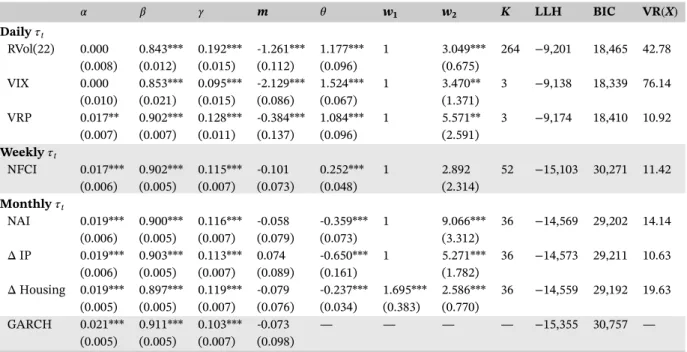
We use the first 20 years of simulated data as the “in-sample” period to obtain QML estimates of the model parameters. Table 1 reports the average bias of the QMLE across the 2,000 Monte Carlo simulations. In panels A/B the innovations Zn,i,tare normally/Studenttdistributed. First, we focus on panel A. In this case the density is correctly specified and the
QMLE is the maximum likelihood estimator. Note that for all parameters exceptw2the average bias is close to zero when
the conditional variance is correctly specified (i.e., with MIDAS lag length ofK = 36 (monthly) andK = 264 (daily)
respectively). Forw2we clearly observe an upward bias.13Based on the 2,000 Monte Carlo replications, we also calculate
12Alternatively, we simulated the intraday returns using a stochastic volatility model that is consistent with our GARCH-MIDAS setting. The
corresponding results, which are very similar to those based on the specification in Equation (21), are presented in Supporting Information Appendix E.
13Figure C.1 in the Supporting Information Appendix compares the histogram of the standardized parameter estimates over the 2,000 Monte Carlo
replications with a standard normal distribution. The figure shows that for all parameters exceptw2the empirical distribution of the parameter estimates
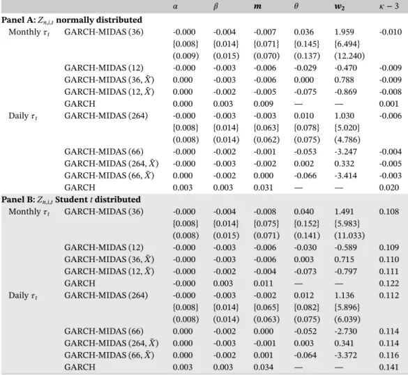
TABLE 1 Monte Carlo parameter estimates
𝛼 𝛽 m 𝜃 w2 𝜅−3
Panel A:Zn,i,tnormally distributed
Monthly𝜏t GARCH-MIDAS (36) -0.000 -0.004 -0.007 0.036 1.959 -0.010 {0.008} {0.014} {0.071} {0.145} {6.494} (0.009) (0.015) (0.070) (0.137) (12.240) GARCH-MIDAS (12) -0.000 -0.003 -0.006 -0.029 -0.470 -0.009 GARCH-MIDAS (36,X̃) 0.000 -0.003 -0.006 0.000 0.788 -0.009 GARCH-MIDAS (12,X̃) 0.000 -0.002 -0.005 -0.075 -0.869 -0.008 GARCH 0.000 0.003 0.009 — — 0.001 Daily𝜏t GARCH-MIDAS (264) -0.000 -0.003 -0.003 0.010 1.030 -0.006 {0.008} {0.014} {0.063} {0.078} {5.020} (0.008) (0.014) (0.062) (0.075) (4.786) GARCH-MIDAS (66) -0.000 -0.002 -0.001 -0.053 -3.247 -0.004 GARCH-MIDAS (264,X̃) -0.000 -0.003 -0.002 0.002 0.332 -0.005 GARCH-MIDAS (66,X̃) 0.000 -0.002 0.000 -0.066 -3.414 -0.003 GARCH 0.003 0.003 0.031 — — 0.020
Panel B:Zn,i,tStudenttdistributed
Monthly𝜏t GARCH-MIDAS (36) -0.000 -0.004 -0.008 0.040 1.491 0.108 {0.008} {0.014} {0.075} {0.152} {5.983} (0.008) (0.015) (0.071) (0.141) (11.033) GARCH-MIDAS (12) -0.000 -0.003 -0.006 -0.030 -0.589 0.109 GARCH-MIDAS (36,X̃) -0.000 -0.003 -0.006 0.003 0.715 0.110 GARCH-MIDAS (12,X̃) -0.000 -0.002 -0.004 -0.073 -0.797 0.111 GARCH -0.000 0.003 0.011 — — 0.122 Daily𝜏t GARCH-MIDAS (264) -0.000 -0.003 -0.002 0.012 1.136 0.112 {0.008} {0.014} {0.065} {0.082} {5.896} (0.008) (0.014) (0.063) (0.075) (6.039) GARCH-MIDAS (66) 0.000 -0.002 0.000 -0.052 -2.730 0.114 GARCH-MIDAS (264,X̃) 0.000 -0.003 -0.001 0.003 0.341 0.114 GARCH-MIDAS (66,X̃) 0.000 -0.002 0.001 -0.064 -3.372 0.116 GARCH 0.003 0.003 0.034 — — 0.141
Note. The table reports the average bias of parameter estimates and the corresponding standard errors across 2,000 Monte Carlo simulations. We provide results for both daily and monthly long-term components. In curly brackets, empirical standard deviations of parameter estimates are reported. Entries in parentheses correspond to the square root of average Wang and Ghy-sels (2015) asymptotic variances. The parameter estimates are based on (the first) 20 years of observations (i.e. the in-sample period). In both long-term components (see Equations (7) and (9)), we choose𝜃=0.3andw1=1. We usem=0.1andw2=4
in the monthly𝜏tandm= −0.1andw2=5in the daily𝜏t. The long-term component is assumed to depend onK=36monthly orK=264daily observations. The covariateXtis modeled as an AR(1) process; that is,Xt=𝜙Xt−1+𝜉t, 𝜉t
i.i.d.
∼ (0, 𝜎2
𝜉), with 𝜙=0.9,𝜎2
𝜉 =0.32for a monthly, and𝜙=0.98,𝜎2𝜉 =0.22for a daily𝜏t. The parameters of the short-term component are in both cases given by𝛼=0.06,𝛽=0.91and𝛾=0. For each model that is estimated based on the true value ofXt, we also incorporate estimations in whichXtis replaced by a noisy proxyX̃t. It is modeled asX̃t=Xt+(0,0.2+0.8|Xt|)in the case of the monthly varying𝜏tandX̃t=Xt+(0,0.5+0.8|Xt|)in the case of a daily varying𝜏t. The column “𝜅−3” presents the mean excess kurtosis of the standardized residuals from each model.
the empirical standard deviation of the estimated parameters. In Table 1 these figures are presented in curly brackets. The numbers in parentheses are the average asymptotic standard errors based on the results in Wang and Ghysels (2015). A comparison of these numbers shows that the asymptotic standard errors are close to the empirical standard deviation of
estimated parameters. The only exception is the specification with monthly𝜏twhere the asymptotic standard errors of
w2appear to be too big. Nevertheless, the overall performance of the asymptotic standard errors is very satisfying. That
is, the Wang and Ghysels (2015) asymptotic standard errors that were derived under the assumption thatXt=
∑J−1
𝑗=0𝜀2t−𝑗
are applicable more generally.
3.2.2
Misspecified models: Bias
Next, we investigate the effect of model misspecification. First, we consider specifications with a smaller lag length than
the true one.14Choosing a lag length that is too small (K =12 for monthly𝜏
torK= 66 for daily𝜏t) does not lead to a
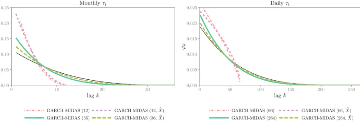
FIGURE 3 Weighting schemes implied by mean parameter estimates. Estimated Beta weighting schemes (see Equation (9)) as implied by the mean parameter estimates reported in Table 1. The green (solid) line corresponds to the case of a correctly specified model, whereas the
red (dot-dashed) line corresponds to a model withKbeing too small. With the brown (long dashed) and purple (short dashed) line, the
corresponding cases of a GARCH-MIDAS with measurement error are reported. The black line shows the true weighting scheme [Colour figure can be viewed at wileyonlinelibrary.com]
bias in the parameter estimates—with the exception ofw2. Now the QMLE ofw2is downwardly biased. As the estimated
weighting schemes in Figure 3 show, the downward bias inw2 translates into biased weighting schemes. Second, we
consider the case of observing the explanatory variableXtwith measurement error. This is a reasonable scenario because
in practice the trueXtis either unknown to or unobservable for the researcher, who will base his analysis on a reasonable
proxy. We denote the proxy byX̃tand specify it asXtplus conditionally heteroskedastic noise. In the case of monthly𝜏t
the noise is given by(0,0.2+0.8|Xt|)and in the case of daily𝜏tby(0,0.5+0.8|Xt|). The average correlation between
XtandX̃tis 68.79%/62.71% for monthly/daily𝜏t. As before, only the QML estimates ofw2appear to be biased whenXtis
replaced withX̃t. Last, we estimate a misspecified one-component GARCH model that is obtained when restricting𝜏tto
be constant. Despite the omitted long-term component, the parameter estimates of𝛼and𝛽are essentially unbiased.
Note that the numbers in panel B of Table 1 are very similar to those in panel A. When replacing the normally distributed
innovations with Studenttdistributed innovations, the density in the maximum likelihood estimation is misspecified
and the estimator is truly QMLE. Nevertheless, this change hardly affects our findings. The only notable difference can be seen in the last column of Table 1, which shows the average excess kurtosis of the fitted standardized residuals. Those residuals are given by𝜀i,t∕
√
̂𝜏tĝi,tfor the GARCH-MIDAS models and by𝜀i,t∕ √
̂
gi,tfor the GARCH model. While the excess
kurtosis is essentially zero in panel A, in panel B there is still excess kurtosis, reflecting the fact that the innovations are
Studenttdistributed.
3.3
Forecast evaluation
Next, we evaluate the forecast performance of the different specifications. Based on the in-sample parameter estimates, we construct OOS volatility forecasts for the remaining 20 years. Keeping the parameter estimates fixed is usually referred
to as a “fixed (forecasting) scheme.”15The forecast performance of the different models will be evaluated over the 2,000
Monte Carlo replications.
We compare the forecast performance of the correctly specified GARCH-MIDAS with all the misspecified models
presented in Table 1. In addition, we consider the two-state MS-GARCH-TVI model that was introduced in Section 2.2.16
3.3.1
MZ regression
We first present the outcomes of MZ regressions. Figure 4 shows theR2
kof MZ regressions for volatility forecasts,hk,t+1|t,
withk = 1,…,22 (i.e., for up to 1 month ahead). Forecast evaluation is based on the noisy proxy𝜀2
k,t+1, whereby the
data generating process is the GARCH-MIDAS with monthly𝜏tand normally distributed innovations. The forecasts are
generated from the correctly specified GARCH-MIDAS model. We present theR2kfor the full OOS period as well as for
15In contrast, in the empirical forecast evaluation in Section 4.4 we apply a “rolling scheme.” As we will discuss below, this is important because it takes
into account the real-time nature of the data and allows for changes in the model parameters.
16In-sample parameter estimates for the MS-GARCH-TVI model can be found in the Supporting Information Appendix, Table B.1. The median estimates
of𝛼and𝛽are close to the true values. The estimates of𝜔1and𝜔2represent a low- and a high-volatility regime. As measured by𝜛=p1,1+p2,2−1, the
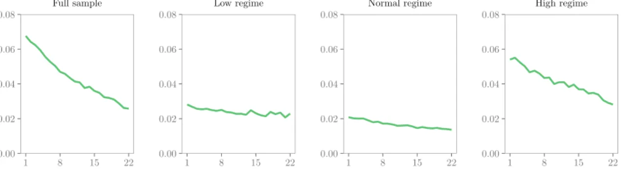
FIGURE 4 MZR2—monthly𝜏
t—evaluation based on𝜀2k,t+1. The figure shows the averageR2kof MZ regressions based on the predictions
from the correctly specified GARCH-MIDAS model over all 2,000 Monte Carlo replications. The true volatility is proxied by𝜀2
k,t+1. Besides the
full out-of-sample period, we consider low-, normal-, and high-volatility regimes. For a definition of the regimes see Section 3.3.1 [Colour figure can be viewed at wileyonlinelibrary.com]
three different volatility regimes:low,normal, andhigh. Volatility regimes are defined as follows. We consider the
empir-ical distribution of daily realized variances during the OOS period. A forecast falls into the low/normal/high-volatility regime if the level of the realized variance on the day the forecast has been issued is below the 25% quantile, between the 25% and 75% quantile, or above the 75% quantile of the empirical distribution. In line with our theoretical result in
Proposition 4, theR2
ks for the full sample are decreasing with increasing forecast horizon. As expected,R
2
1 is below the
upper bound of one-third (see Equation (15)). Among the three regimes, we observe the highestR2
ks in the high-volatility
regime. Clearly, the highR2
ks in the high-volatility regime do not reflect an improved absolute forecast performance but
rather an improved relative forecast performance. Further, note that for almost all forecast horizons theR2
ks in the full
sample are higher than in each subsample.
For empirical applications, cumulative volatility forecasts are of greater importance thank-step-ahead forecasts. Hence
in Figure 5 we present theR2
1∶kof MZ regressions for cumulative volatility forecasts,h1:k,t+1|t, withk=1,…,22. Note that,
by construction, the volatility forecasts are nonoverlapping. We now present forecasts from the correctly specified and the misspecified GARCH-MIDAS models as well as from the MS-GARCH-TVI and the nested GARCH. Forecast evaluation
is based on the precise proxy RV1:k,t+1. Panels (a)/(b) show the results for monthly/daily𝜏t. Based on Figure 5, we are able
to rank the different models' forecast performance. While the performance of all GARCH-MIDAS models is essentially
indistinguishable, the one-component GARCH and the MS-GARCH-TVI models lead to a lowerR2
1∶k. Differences between
models are most pronounced in the low and normal regime.
3.3.2
Model confidence sets
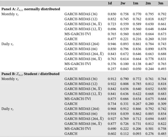
Next, we formally test for superior predictive ability. We base our analysis on the MCS approach introduced by Hansen et al. (2011). Following the arguments in Patton (2011), we use the QLIKE loss as the evaluation criterion. For a
k-step-ahead volatility forecast, the QLIKE is defined as
QLIKE ( 𝜎2 k,t+1,hk,t+1|t ) =𝜎k2,t+1∕hk,t+1|t−ln ( 𝜎2 k,t+1∕hk,t+1|t ) −1. (22)
The QLIKE is the only robust loss function that depends solely on the standardized forecast error,𝜎2
k,t+1∕hk,t+1|t. As
discussed in Patton (2011), the QLIKE is less sensitive with respect to extreme observations than the squared error loss. Further, it can be shown that the moment conditions required for Diebold and Mariano (1995) or Giacomini and White (2006) type tests are weaker under QLIKE than under squared error loss (see Patton, 2006).
We consider the following forecasting schemes. Based on the information available at the last day of the current month, cumulative volatility forecasts are computed for horizons of 1 day (1d), 2 weeks (2w), and 1 month (1m), as well as fore-casts of volatility in 2 months (2m) and 3 months (3m). Whenever the forecast horizon is longer than the frequency of the long-term component, the optimal forecast requires predicting the long-term component. Instead, we simply fix the
long-term component at its current level (see Section 2.4). Forecast evaluation is now based on the precise proxyRV1:k,t+1.
FIGURE 5 MZR2
1∶k—monthly and daily𝜏t—evaluation based on RV1:k,t+1: (a) monthly𝜏t; (b) daily𝜏t. For each model the figure shows
the averageR2
1∶kof the MZ regressions over the 2,000 Monte Carlo replications. The true volatility is proxied by RV1:k,t+1. The upper/lower
panels display the case of monthly/daily long-term components. Besides the full out-of-sample period, we consider low-, normal-, and high-volatility regimes. For a definition of the regimes see Section 3.3.1 [Colour figure can be viewed at wileyonlinelibrary.com]
di,𝑗(s,k) =QLIKE ( RV1∶k,t+s, ̂h1(i∶)k,t+s|t ) −QLIKE ( RV1∶k,t+s, ̂h1(𝑗∶)k,t+s|t )
as the difference in the QLIKE loss of modelsiandj. For example, whens= 1 andk ∈ {1,5,22}the forecastĥ(1i∶)k,t+s|t denotes the cumulative forecast for the first (1d), the first 5 (1w), or all 22 (1m) days in the following month while for
s ∈ 2,3 andk = 22 we obtain the forecast for 2 (2m) and 3 (3m) months in the future. We compute the average loss
difference,d̄i,𝑗, and calculate the test statistic:
ti𝑗=d̄i,𝑗∕ √
̂
var(d̄i,𝑗) for all i, 𝑗∈. (23)
The MCS test statistic is then given byT = max
i,𝑗∈|ti,𝑗|and has the null hypothesis that all models have the same
expected loss. Under the alternative, there is some modelithat has an expected loss greater than the expected loss of all
other models𝑗∈∖i. If the null hypothesis is rejected, the worst-performing model is eliminated. The test is performed
iteratively, until no further model can be eliminated. We denote the final set of surviving models byMCS. This final set
contains the best forecasting model with confidence level 1−𝜈. We set𝜈 = 0.1. This choice is common practice in the

![TABLE 3 LM test for misspecification of GJR-GARCH(1 , 1) X t VIX RVol NFCI NAI Δ IP Δ Hous K = 1 76 .28 [ <0.01] 14 .38[<0.01] 22 .54[<0.01] 15 .25[<0.01] 7 .99[ <0.01] 0 .18[0.67] K = 2 84 [<0.01].05 19 [<0.01].03 24 [<0.01].05 17](https://thumb-us.123doks.com/thumbv2/123dok_us/9017854.2799578/18.892.437.823.70.141/table-test-misspecification-gjr-garch-rvol-nfci-hous.webp)