Forecasting Nord Pool day-ahead prices with Python
Tarjei Kristiansen
SINTEF Energy Research
Abstract
Price forecasting accuracy is crucially important for electricity trading and risk management. This paper discusses building multiple Nord Pool forecasting models for hourly day-ahead prices, which utilize the Python programming language. The autoregressive models are based on Kristiansen (2012) and the dataset ranges from January 2004 to May 2011. The targets (i.e. dependent variables) are the hourly day-ahead prices for a certain hour during the day and the features (i.e. independent variables) are the prices for the same hour the previous two days and the previous week, the maximum price for the previous day, and four weekday dummy variables including the demand and wind for the actual hour. We use an ordinary least squares (OLS) regression framework with cross-validation to test the models. Next, we use regularized regressions including Ridge and Lasso, and finally we use a Keras neural network. Evaluations of the models using the mean absolute percentage error (MAPE) criterion, R-square and scatterplots, show that the MAPE of the OLS, Ridge and Lasso regressions are 7.09%, 7.11% and 7.07%, respectively, the MAPE of the Keras neural network is 6.53%, and the R-square of the regressions and the neural network are 0.892 and 0.904, respectively. The results demonstrate that the autoregressive exogenous models perform well, are user-friendly and could add value for market players.
Keywords: autoregressive exogenous model, Nordic power market, price forecasting, Python
language, regressions, neural network. 1. Introduction
Price forecasting is a crucially important activity for electricity trading and risk management. Even though day-ahead price forecasts are commercially available from several analytics service providers, it is more advantageous for market players to build their own in-house price forecasting models and apply them to the input data. The literature is limited, however, on how to develop practical implementable models with user-friendly software such as the Python programming language.
In this paper, we present an autoregressive (ARX) model with exogenous variables based on Weron and Misiorek (2008) to compute price predictions for all 24 hours of a given day. Kristiansen (2012) modified their model by reducing the estimation parameters (from 24 sets to 1) and including Nordic demand and Danish wind power as the exogenous variables. Prices were modelled across all hours in the analysis period rather than across each single 24 hour, which reduced the number of models and estimation parameters. Input data such as historic Nord Pool day-ahead prices, demand and Danish wind output are publicly available
information. We apply our ARX model to a dataset from January 2004 to May 2011 (see the Appendix for the Python source code).
2. Day-ahead price forecasting methods
Weron (2006), which reviews the popular approaches used to model and forecast day-ahead electricity prices, finds that time series models are one of the most powerful model groups. Weron (2006 and 2008) finds that model specifications for each hour separately have better forecasting properties than model specifications common for all hours. Model specifications include Autoregressive (AR) models, Autoregressive Moving Average (ARMA), Autoregressive Integrated Moving Average (ARIMA) and seasonal ARIMA models (Contreras et al., 2003; Zhou et al., 2006), autoregressions with heteroskedastic (Garcia et al. 2005) or heavy-tailed innovations (Weron, 2008), AR models with exogenous (fundamental) variables–dynamic regression (or ARX) and transfer function (or ARMAX) models (Conejo et al., 2005), vector auto regressions with exogenous effects (Panagiotelis and Smith, 2008), threshold AR and ARX models (Misiorek et al., 2006), regime-switching regressions with fundamental variables (Karakatsani and Bunn, 2008) and mean-reverting jump diffusions (Knittel and Roberts, 2005).
Starting in the 1990s, artificial intelligence (AI) has been deployed in load forecasting, but the literature on the application of artificial intelligence to electricity price forecasting is relatively limited. Wang and Ramsay (1998) apply neural networks to forecast the system marginal price in England and Wales. They achieve a mean absolute percentage error of around 9% for weekends and 12% for public holidays. Gareta et al. (2006) describe the application of AI to electricity price forecasting. The authors utilize neural networks to forecast hourly prices. The main advantage of neural networks is their flexible nonlinear modelling including complexity, a particularly useful characteristic for markets where prices exhibit volatility, spikes and seasonality, i.e. electricity markets. Ramos and Liu (2012) provide an overview of various AI techniques in power systems and energy markets. Chaabane (2014), applies Auto-Regressive Fractionally Integrated Moving Average (ARFIMA) and a neural network model to forecast Nord Pool power prices. The author tests the approach on 100 data points in November 2012 and achieves a mean absolute percentage error of 6.5%.
Weron (2014), a comprehensive overview of electricity price forecasting methods, points out that AI models are flexible and can handle complexity. Artificial neural networks (ANNs) can be classified in two groups: 1) feed forward networks without loops, and 2) recurrent (i.e. feedback) networks. The first group is preferred in forecasting and the latter is preferred for classification and categorization. ANN models can also be used for prediction intervals (PIs). ANN-based models have gained popularity because they can map any nonlinear function with a high degree of accuracy. They are also capable of including exogenous factors.
Singh et al. (2017), describe an application of a neural network to the price forecasting of New South Wales day-ahead electricity prices. The authors describe the process of price forecasting as a signal processing problem with proper estimation of model parameters and uncertainties. They propose a generalized neuron model where the pre-processing of parameters is performed by using wavelet transform and the free parameters are tuned by using an
environment adaption method algorithm to increase the generation ability and the efficacy of the model.
3. Regressions in the Python language
Python is an interpreted, high-level programming language for general-purpose programming (Python, 2018). In the Python language ordinary least squares (OLS) regression framework, the dependent variable is named the target and the independent variables are the features. The intercept and the slopes of the regression are parameters. The parameters are chosen by defining an error function for a given line (in case of a single feature) and choosing the line that minimizes the error function. A loss function is defined which, in the case of OLS, minimizes the squares of residuals. The regression estimates a coefficient ai for each feature variable. Large coefficients resulting in overfitting can be mitigated by regularization; the large coefficients are penalized.
In a Ridge regression, the loss function is expressed as: OLS loss function ∑ ,
where αis the parameter to be selected and which controls model complexity. If α is zero, the loss function equals the OLS loss function and there is potentially overfitting, whereas a high
α can result in underfitting.
In a Lasso regression, the loss function is expressed as: OLS loss function ∑ | |.
The Lasso regression can be used to select the significant features of a dataset. The coefficients of less significant features are set to zero.
The dataset used to learn the patterns is called the training set and the training error is the loss function. If the model overfits on the training data, it may not generalize well on future data because model performance depends on how the data are split. To avoid overfitting, cross-validation (CV) may be utilized. In this framework, various folds or splits of data may be applied, but more folds are computationally expensive. CV estimates the error by removing a group of samples from the training set and trains the model on the remaining set.
4. Autoregressive exogenous models
There are some naive approaches to forecasting day-ahead prices. The similar-day approach is based on searching historical data for days with similar characteristics to those of the forecasted day (Weron, 2006). Similar characteristics may include day of the week, day of the year or even weather properties. The price of a similar day is considered as the forecast. Instead of a single similar-day price, the forecast can be a linear combination or a regression procedure that includes several similar days. An example of a simple, yet in some cases relatively powerful, implementation of the similar-day or naive method is a Monday similar to the Monday of the previous week and applying the same rule for Saturdays and Sundays (Weron,
Around 60% of Nordic power generation is hydropower. Therefore, the supply side is predominantly weather dependent. A rationale for a Nord Pool forecasting model is that the day-ahead price should reflect all available information discounted in the historic prices. Likewise, the hourly profile of the day-ahead price should reflect the demand profile over the course of the day. The demand is typically lower in off-peak hours (hours 0–8 and 20–24) and on weekends. Typically, the price level is similar to the previous day’s price level adjusted for any changes in water values. Since hydropower generation can quickly ramp up production and meet demand, prices are therefore normally smooth and exhibit smaller differences between peak and off-peak prices compared to thermal systems which must consider the start/stop costs. A regression model is more suitable for a market dominated by hydropower than a pure thermal power system.
Weron and Misiorek (2008) used Nord Pool data from 1998 to 1999 (a period with high water reservoir levels) and from 2003 to 2004 (a period with low water reservoir levels) to evaluate their proposed model. In this paper, we use data from 2004 to 2011 (years with both dry and wet periods). Unlike Weron and Misiorek (2008), which use temperatures, we use historical demand, and include Danish wind power and total Nordic demand.
The natural logarithmic transformation has been applied to the price, pt=ln(Pt), the load
zt=ln(Zt) and the wind wt=ln(Wt) to attain a more stable variance. In Weron and Misiorek (2008), the authors argue that since each hour displays a rather distinct price profile reflecting the daily variation of demand, costs and operational constraints, the modelling should be implemented across all 24 hours, thus producing 24 sets of parameters. Instead, we implement the model across all hours in the analysis period, which produces only one set of parameters. We note that operational forecasting should use forecasts for demand and wind power for the next day. We use historical data in the back testing of our model.
The weekly seasonal behaviour is captured by a combination of (1) the autoregressive structure of the models, and (2) the daily dummy variables. The ln-price pt depends on the ln-prices for the same hour on the previous two days, and the previous week. This choice of model variables is motivated by the significance of the coefficients found by Weron and Misiorek (2008), who also use the minimum of all hourly prices on the previous day, which creates the desired link between bidding and price signals from the entire day. Instead, we choose the maximum price on the previous day as in Kristiansen (2012). We use four dummy variables (Monday, Friday, Saturday and Sunday) to differentiate between the two weekend days, the first business day of the week, the last business day of the week and the remaining business days.
The basic autoregressive model structure is formulated as:
(1) where lagged ln-prices pt-24, pt-48 and pt-168 account for the autoregressive effects of the previous days (the same hour yesterday, two days ago and one week ago, respectively), mpt creates the link between bidding and price signals from the previous day (the maximum of the previous day’s 24 hourly ln-prices), dummy variables Dmon, Dfri, Dsat and Dsun (account for the weekly seasonality), β’s are the regression coefficients for the lagged prices, α is the regression coefficient for the maximum hourly price on the previous day, d's are the regression coefficients for the weekday dummy variables, γis the regression coefficient for the load and
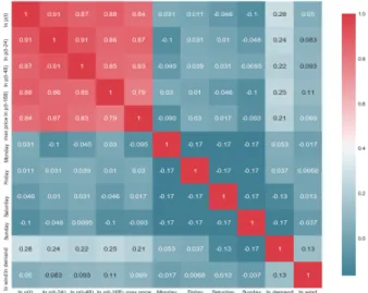
δ is the regression coefficient for the wind. We assume εt's are independent and identically distributed with zero mean and finite variance. The model formulation states that tomorrow’s hourly price (forecasted) depends on the hourly day-ahead the previous same 24-hour, 48-hour and 168-hour including the hourly forecasted Nordic demand and Danish wind generation for the day-ahead. In addition, there is a link between the day-ahead price and the previous day’s price level, including links between different weekdays. Figure 4.1 shows the correlation map for the time series data. The lagged prices (t-24, t-48 and t-168) and maximum price level on the previous day correlate highly to the price at hour t, and demand has a higher correlation than the weekdays and wind.
Figure 4.1. Correlation for the time series data (red-high, blue-low). 5. Regression case studies
The next section describes using available Python software to obtain various regressions. 5.1. Ordinary least squares regression
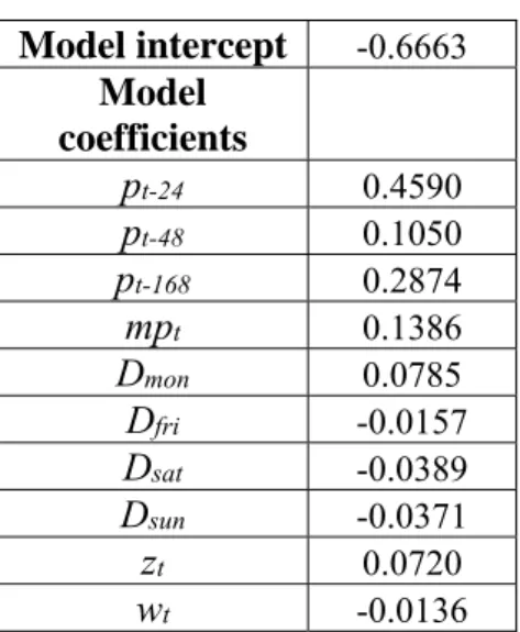
Table 5.1 shows the model intercept and coefficients of an ordinary least squares regression. We note that the price for a certain hour today depends mainly on the previous day’s and previous week’s same hourly price (i.e. 168 hours previous price) as these variables have the largest regression coefficients. The R-square for the regression is 0.892, the Augmented Dickey Fuller (ADF) statistic is -6.43 and the p-value is 0.0000. The ADF tests the null hypothesis that a unit root is present in the time series data.
Model intercept -0.6663 Model coefficients pt-24 0.4590 pt-48 0.1050 pt-168 0.2874 mpt 0.1386 Dmon 0.0785 Dfri -0.0157 Dsat -0.0389 Dsun -0.0371 zt 0.0720 wt -0.0136
Table 5.1. Model intercept and coefficients for OLS regression.
The critical values for a hypothesis test are dependent on a test statistic and the significance level. A significance level of 0.04 implies that the null hypothesis is rejected 4% of the time when it is in fact true. Thus, critical values are basically cut-off values that define regions where the test statistic is unlikely to be false. As shown in Table 5.2, the ADF statistic (-6.43) is lower than the critical values so the series exhibits stationarity.
Critical values
1%: -3.43 5%: -2.862 10%: -2.567 Table 5.2. Critical values.
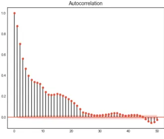
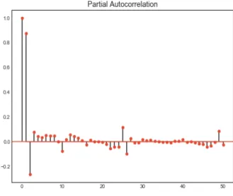
Often, the connection between two random variables in a given stochastic process at different points in time is of interest. One way to measure a linear relationship is with the autocorrelation function (ACF), which measures the correlation between the two variables. The partial autocorrelation function (PACF), which yields the partial correlation for time series of shorter lags can be used to determine the order of the autoregressive model.
Therefore, we apply the ACF and PACF with 50 time lags on the residuals and the squared residuals as shown in Figure 5.1 through Figure 5.4. The ACF residual tails off to 0 after about 45 lags whereas the ACF squared residual tails off to 0 after about 30 lags (Figure 5.1 and Figure 5.2). The PACF tails off for lag 4 for both the residual and the squared residual (Figure 5.3 and Figure 5.4).
Figure 5.1. The autocorrelation function for the residuals.
Figure 5.3. The partial autocorrelation function for the residuals.
Figure 5.4. The partial autocorrelation function for the squared residuals.
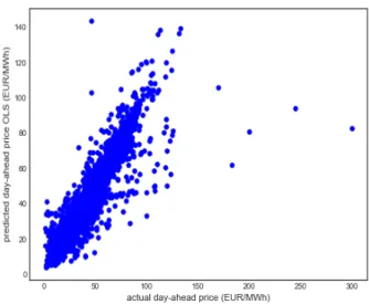
Figure 5.5 shows the scatterplot of predicted ahead (EUR/MWh) against the actual day-ahead price (EUR/MWh) for an OLS. Note the strong correlation and confirmation of the model’s relatively high R-square value. To measure the performance of the models we use the mean absolute percentage error (MAPE) defined as the average absolute difference between the actual value and the forecast value divided by the actual value. We transform the right-hand side of Eq. (1) by taking the exponential function of it to recreate the original prices from the natural logarithm of prices. The model's MAPE is 7.09%.
Figure 5.5. Scatterplot of predicted day-ahead price (EUR/MWh) vs actual day-ahead price (EUR/MWh) for the ordinary least square regression.
We also run the CV with 10 folds; Table 5.3 lists the R-square values.
fold 1 0.5414 fold 2 0.7295 fold 3 0.8423 fold 4 0.8443 fold 5 0.8059 fold 6 0.7972 fold 7 0.7899 fold 8 0.4582 fold 9 0.6014 fold 10 0.8530 average 0.7263
Table 5.3. R-square values for 10 folds in the CV. 5.2. Ridge regression
Next, we perform a Ridge regression with an α parameter of 0.005. Table 5.4 reports that the R-square for the regression is 0.892.
Model intercept -0.6721 Model coefficients pt-24 0.4459 pt-48 0.1139 pt-168 0.2865 mpt 0.1429 Dmon 0.0773 Dfri -0.0160 Dsat -0.0392 Dsun -0.0376 zt 0.0728 wt -0.0135
Table 5.4. Model intercept and coefficients for the Ridge regression.
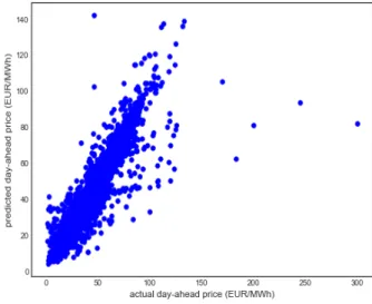
Figure 5.6 shows the scatterplot of predicted day-ahead (EUR/MWh) against actual day-ahead price (EUR/MWh) for the Ridge regression. The model’s MAPE is 7.11%.
Figure 5.6. Scatterplot of predicted day-ahead price (EUR/MWh) vs actual day-ahead price (EUR/MWh) for the Ridge regression.
5.3. Lasso regression
Finally, we perform a Lasso regression with an α parameter of 1.662*10-6. Table 5.5 reports
Model intercept -0.6549 Model coefficients pt-24 0.4591 pt-48 0.1035 pt-168 0.2880 mpt 0.1385 Dmon 0.0782 Dfri -0.0142 Dsat -0.0374 Dsun -0.0356 zt 0.0710 wt -0.0133
Table 5.5. Model intercept and coefficients for the Lasso regression.
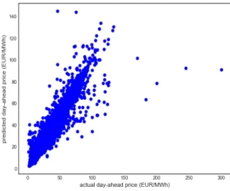
Figure 5.7 shows the scatterplot of predicted day-ahead (EUR/MWh) against actual day-ahead price (EUR/MWh) for the Lasso regression. The model’s MAPE is 7.07%. Figure 5.8 shows the model feature selection in the Lasso regression. The lagged prices pt-24 and pt-168 are the most influential features.
Figure 5.7. Scatterplot of predicted day-ahead price (EUR/MWh) vs actual day-ahead price (EUR/MWh) for the Lasso regression.
Figure 5.8. Feature model selection in the Lasso regression. 6. Keras neural network
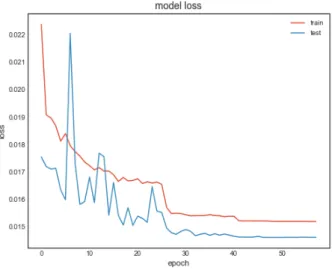
Keras is a high-level neural networks API (Keras, 2018) written in the Python language. Keras facilitates the organization of layers, with Sequential being the simplest model. We use the Sequential model with mean squared error (MSE) as a loss function, a batch size of 32 and set the number of epochs (a measure of the number of times all training vectors are used once to update the weights) to 100. Running the simulation results in a MAPE of 6.53% and a R-square of 0.904. Figure 6.1 shows a scatterplot of the predicted day-ahead price vs the actual day-ahead price for the Keras neural network, Figure 6.2 shows the model loss function for the training and test sets as a function of epochs and Figure 6.3 shows mean squared errors, mean absolute error and mean absolute percentage errors as a function of epochs.
Figure 6.1. Scatterplot of predicted day-ahead price (EUR/MWh) vs actual day-ahead price (EUR/MWh) for the Keras neural network.
Figure 6.2 The model loss function for the training and test sets as a function of epochs.
Figure 6.3. Mean squared error, mean absolute error and mean absolute percentage error as a function of epochs.
7. Conclusions
This paper presented a simple, user-friendly regression model for the Nord Pool power market by utilizing various regressions available including a neural network written in Python programming language. The model implementation was similar to that of Kristiansen (2012). An ordinary least squares regression yielded a MAPE of 7.09%, which was is comparable to Kristiansen (2012) which had a MAPE of 8% for the full analysis period (2004–2011) and the MAPE of 5% for the out-of-sample period (2004–2006). A Ridge regression yielded a MAPE of 7.11%. Likewise, a Lasso regression yielded a MAPE of 7.07%. A Keras neural network regression which yielded a MAPE of 6.53%. The R-squares for the regressions and the neural network were 0.892 and 0.904, respectively. The results for the regressions were similar to the
OLS in Kristiansen (2012) but applying a Keras neural network regression improved the model’s accuracy because the number of training parameters was increased.
This paper demonstrated how multiple, relatively accurate forecasting models for Nord Pool prices can be implemented easily in Python. Building their own in-house price forecasting models could give traders an edge over the competition in electricity markets.
References
Chaabane N. (2014): A hybrid ARFIMA and neural network model for electricity price prediction, Electrical Power and Energy Systems 55, pp. 187–194.
Conejo A.J., Contreras J., Espınola R. and Plazas M.A. (2005): Forecasting electricity prices for a day-ahead pool-based electric energy market, International Journal of Forecasting, vol. 21 (3), pp. 435-462.
Contreras J., Espınola R., Nogales F.J. and Conejo A.J. (2003): ARIMA models to predict next-day electricity prices, IEEE Transactions on Power Systems, vol. 18 (3), pp. 1014-1020. Garcia R.C., Contreras J., van Akkeren M. and Garcia J.B.C. (2005): A GARCH forecasting
model to predict day-ahead electricity prices, IEEE Transactions on Power Systems, vol. 20 (2), pp. 867-874.
Gareta G., Romeo L. M. and Gil. A. (2006): Forecasting of electricity prices with neural networks, Energy Conversion and Management 47, pp. 1770–1778.
Karakatsani N. and Bunn D. (2008): Forecasting electricity prices: the impact of fundamentals and time-varying coefficients, International Journal of Forecasting, vol 24 (4), pp. 764-785.
Keras, documentation, https://keras.io, accessed on Jan 18, 2018.
Knittel C.R. and Roberts M.R. (2005): An empirical examination of restructured electricity prices, Energy Economics, vol. 27 (5), pp. 791-817.
Kristiansen T. (2012): Forecasting Nord Pool day-ahead prices with an autoregressive model, Energy Policy, vol. 49, pp. 328-332, Oct.
Misiorek A., Truck S. and Weron R. (2006): Point and interval forecasting of spot electricity prices: linear vs. non-linear time series models, Studies in Nonlinear Dynamics and Econometrics 10 (3).
Panagiotelis A. and Smith M. (2008): Bayesian forecasting of intraday electricity prices using multivariate skew-elliptical distributions, International Journal of Forecasting, vol. 24 (4), pp. 710-727.
Python, https://www.python.org/, accessed on Jan 18, 2018.
Ramos C. and Liu C. (2012): AI in Power Systems and Energy Markets, Intelligent Systems, IEEE, May.
Singh N., Mohanty S. R. and Shukla R. D. (2017): Short term electricity price forecast based on environmentally adapted generalized neuron, Energy, Volume 125, 15 April, pp. 127-139.
Wang, A.J. and Ramsay B. (1998): A neural network based estimator for electricity spot-pricing with particular reference to weekend and public holidays, Neurocomputing, Volume 23, Issues 1–3, 7 December, pp. 47-57.
Weron R. (2006): Modeling and Forecasting Electricity Loads and Prices: A Statistical Approach, Wiley, Chichester.
Weron R. (2008): Forecasting wholesale electricity prices: a review of time series models. In: Financial Markets: Principles Of Modeling, Forecasting and Decision-Making, W. Milo, P. Wdowinski (Eds.), FindEcon Monograph Series, WU L, Lodz.
Weron R. (2014): Electricity price forecasting: A review of the state-of-the-art with a look into the future, International Journal of Forecasting, 30, pp. 1030–1081.
Weron R. and Misiorek A. (2008): Forecasting spot electricity prices: a comparison of parametric and semiparametric time series models, International Journal of Forecasting, 24, pp. 744-763.
Zhou M., Yan Z., Ni Y., Li G. and Nie Y. (2006): Electricity price forecasting with confidence-interval estimation through an extended ARIMA approach, IEE Proceedings Generation, Transmission and Distribution, vol. 153 (2), pp. 233-238.
Appendix A: Python source code for the models and analysis
PYTHON CODE FOR CORRELATION MAP, ADF TEST AND PACF PLOTS
# correlation map, ADF test, ACF and PACF plots import pandas as pd
import numpy as np
import matplotlib.pylab as plt
from statsmodels.tsa.stattools import adfuller import statsmodels.tsa.api as smt
from data_visualization import plot_correlation_map from sklearn import linear_model
# read the time series data from a file named Nord Pool spot prices 2004-2011 max.csv
# column headers are date, ln p(t), ln p(t-24), ln p(t-48), ln p(t-168), max price, Monday, Friday, Saturday, Sunday, ln demand, ln wind
data = pd.read_csv(r'C:\time series\Nord Pool spot prices 2004-2011 max.csv',sep=';',index_col='date',parse_dates=['date'])
# exclude NA data.dropna()
# define all features
X=data.drop('ln p(t)', axis=1).values # define target
y=data['ln p(t)'].values # linear regression
reg_all.fit(X,y) # predict y
y_pred = reg_all.predict(X)
# difference between actual and predicted values, take exponential because regression is on ln of time series
residuals=-np.exp(y)+np.exp(y_pred) # show correlation map
plot_correlation_map(data) # AD Fuller test statistic result = adfuller(y)
print('ADF Statistic: %f' % result[0]) print('p-value: %f' % result[1])
print('Critical Values:')
for key, value in result[4].items(): print('\t%s: %.3f' % (key, value))
# graph residuals of ACF and PACF with lags 50 and alpha=0.5 print('residuals')
smt.graphics.plot_acf(residuals, lags=50,alpha=0.05) plt.show()
smt.graphics.plot_pacf(residuals, lags=50,alpha=0.05) plt.show()
# graph squared residuals of ACF and PACF with lags 50 and alpha=0.5 print('squared residuals')
smt.graphics.plot_acf(residuals*residuals, lags=50, alpha=0.05) plt.show()
smt.graphics.plot_pacf(residuals*residuals, lags=50,alpha=0.05) plt.show()
PYTHON CODE FOR OLS, RIDGE AND LASSO REGRESSIONS
# OLS, Ridge and Lasso regressions import pandas as pd
import numpy as np
import matplotlib.pylab as plt from sklearn import linear_model
from sklearn.model_selection import train_test_split from sklearn.model_selection import cross_val_score from sklearn.linear_model import Ridge, Lasso
import math
# calculation of mean absolute percentage error (MAPE) def mape(y_true,y_pred,n):
tmp = 0.0
y_true=np.exp(y_true) y_pred=np.exp(y_pred)
for i in range(0,n):
tmp += math.fabs(y_true[i]-y_pred[i])/y_true[i] return (tmp/n)
# read time series
data = pd.read_csv(r'C:\time series\Nord Pool spot prices 2004-2011 max.csv',sep=';',index_col='date',parse_dates=['date']) # exclude NAs data.dropna() # define features X=data.drop('ln p(t)', axis=1).values # define target y=data['ln p(t)'].values # name features
names = data.drop('ln p(t)', axis=1).columns
# define train and test sets, 30% to be included in test set, random_state used to initializing random number generator
X_train, X_test, y_train, y_test = train_test_split(X, y, test_size = 0.3, random_state=42)
# define the linear regression
reg_all= linear_model.LinearRegression() # perform OLS regression
reg_all.fit(X_train,y_train) # predict dependent variable y_pred = reg_all.predict(X_test)
# The coefficients of the OLS regression
print("OLS model intercept:", reg_all.intercept_) print('OLS coefficients') print(pd.Series(reg_all.coef_, names)) print('score OLS') print(reg_all.score(X_test, y_test)) # scatterplot of OLS plt.scatter(np.exp(y_test),np.exp(y_pred),color='blue') plt.xlabel('actual day-ahead price (EUR/MWh)')
plt.ylabel('predicted day-ahead price OLS (EUR/MWh)') plt.show()
# OLS MAPE
print('OLS MAPE')
print(mape(y_test,y_pred,len(y_pred)))
# cross validation of data to take into account that model performance is dependent on way the data is split
print('cv results') print(cv_results)
print(np.mean(cv_results)) # regularization
# Ridge regression
ridge = Ridge(alpha=0.005, normalize=True) ridge.fit(X_train, y_train)
ridge_pred = ridge.predict(X_test) print('Ridge score')
print(ridge.score(X_test, y_test)) # The Ridge coefficients
print("Ridge model intercept:", ridge.intercept_) print('Ridge Coefficients')
print(pd.Series(ridge.coef_, names)) # scatterplot of Ridge
plt.scatter(np.exp(y_test),np.exp(ridge_pred),color='blue') plt.xlabel('actual day-ahead price (EUR/MWh)')
plt.ylabel('predicted day-ahead price (EUR/MWh)') plt.show()
# Ridge MAPE
print('Ridge MAPE')
print(mape(y_test,ridge_pred,len(ridge_pred))) # Lasso
lasso = Lasso(alpha=1.66225173363e-06, normalize=True) lasso.fit(X_train, y_train)
lasso_pred = lasso.predict(X_test) print('Lasso score')
print(lasso.score(X_test, y_test)) # The Lasso coefficients
print("Lasso model intercept:", lasso.intercept_) print('Lasso coefficients')
print(pd.Series(lasso.coef_, names)) # scatterplot of Lasso
plt.scatter(np.exp(y_test),np.exp(lasso_pred),color='blue') plt.xlabel('actual day-ahead price (EUR/MWh)')
plt.ylabel('predicted day-ahead price (EUR/MWh)') plt.show()
# Lasso MAPE
print('Lasso MAPE')
print(mape(y_test,lasso_pred,len(lasso_pred))) #important Lasso coefficients
names = data.drop('ln p(t)', axis=1).columns lasso = Lasso(alpha=0.1)
lasso_coef = lasso.fit(X, y).coef_
_ = plt.plot(range(len(names)), lasso_coef)
_ = plt.xticks(range(len(names)), names, rotation=60) _ = plt.ylabel('Lasso coefficients')
plt.show()
PYTHON CODE FOR KERA NEURAL NETWORK
# Keras neural network import pandas as pd import numpy as np
import matplotlib.pylab as plt
from sklearn.model_selection import train_test_split from sklearn.metrics import r2_score
from keras.models import Sequential from keras.layers import Dense
from keras.callbacks import EarlyStopping, ModelCheckpoint, ReduceLROnPlateau
import math
# calculation of mean absolute percentage error (MAPE) def mape(y_true,y_pred,n): tmp = 0.0 y_true=np.exp(y_true) y_pred=np.exp(y_pred) for i in range(0,n): tmp += math.fabs(y_true[i]-y_pred[i])/y_true[i] return (tmp/n)
# read the data
data = pd.read_csv(r'C:\time series\Nord Pool spot prices 2004-2011 max.csv',sep=';',index_col='date',parse_dates=['date']) # exclude NAs data.dropna() # define features X=data.drop('ln p(t)', axis=1).values # define target y=data['ln p(t)'].values # name features
names = data.drop('ln p(t)', axis=1).columns
# define train and test sets, 30% to be included in test set, random_state used to initializing random number generator
X_train, X_test, y_train, y_test = train_test_split(X, y, test_size = 0.3, random_state=42)
# define the sequential model with two-classification regression with 10 features
# the hidden dense layer has 64 neurons model = Sequential()
model.add(Dense(64,activation='relu',input_dim=10)) model.add(Dense(1))
# summarize the model model.summary()
# fix random seed for reproducibility seed = 7
np.random.seed(seed)
# early stopping criterion
earlyStopping = EarlyStopping(monitor='val_loss', patience=10, verbose=0, mode='min')
# save model
mcp_save = ModelCheckpoint('.mdl_wts.hdf5', save_best_only=True, monitor='val_loss', mode='min')
# Reduce learning rate when a metric has stopped improving
reduce_lr_loss = ReduceLROnPlateau(monitor='val_loss', factor=0.1, patience=7, verbose=1, epsilon=1e-4, mode='min')
# training of the neural network with 30% of the data to use as held-out validation data
history=model.fit(X_train, y_train, batch_size=32, epochs=100, verbose=1, callbacks=[earlyStopping, mcp_save, reduce_lr_loss],
validation_split=0.3,validation_data=(X_test,y_test)) # forecast
predictions = model.predict(X_test) #calculate R-square
print('R-square')
print(r2_score(y_test, predictions, sample_weight=None, multioutput='uniform_average')) # MAPE print('MAPE') print(mape(y_test,predictions,len(predictions))) #scatter plot plt.scatter(np.exp(y_test),np.exp(predictions),color='blue') plt.xlabel('actual day-ahead price (EUR/MWh)')
plt.ylabel('predicted day-ahead price (EUR/MWh)') plt.show() plt.plot(history.history['loss']) plt.plot(history.history['val_loss']) plt.title('model loss') plt.ylabel('loss') plt.xlabel('epoch')
plt.legend(['train', 'test'], loc='upper right') plt.show()
# plot performance metrics
plt.plot(history.history['mean_squared_error']) plt.plot(history.history['mean_absolute_error'])
plt.plot(history.history['mean_absolute_percentage_error']) plt.ylabel('measure')
plt.xlabel('epoch')
plt.legend(['mean_squared_error',
'mean_absolute_error','mean_absolute_percentage_error'], loc='upper right')