Internet traffic modeling and forecasting using non-linear time series model GARCH

(1)

INTERNET TRAFFIC MODELING AND FORECASTING

USING NON-LINEAR TIME SERIES MODEL GARCH

by

CHAOBA NIKKIE ANAND

M.E., Bangalore University, India, 2004

A THESIS

submitted in partial fulfillment of the

requirements for the degree

MASTER OF SCIENCE

Department of Electrical and Computer Engineering

College of Engineering

KANSAS STATE UNIVERSITY

Manhattan, Kansas

2009

Approved by:

Major Professor Caterina Scoglio

(2)

Copyright

Chaoba Nikkie Anand

(3)

Abstract

Forecasting of network traffic plays a very important role in many domains such as con-gestion control, adaptive applications, network management and traffic engineering. Char-acterizing the traffic and modeling are necessary for efficient functioning of the network. A good traffic model should have the ability to capture prominent traffic characteristics, such as long-range dependence (LRD), self-similarity, and heavy-tailed distribution. Be-cause of the persistent dependence, modeling LRD time series is a challenging task. In this thesis, we propose a non-linear time series model, Generalized AutoRegressive Conditional Heteroskedasticity (GARCH) of order p and q, with innovation process generalized to the class of heavy-tailed distributions. The GARCH model is an extension of the AutoRegres-sive Conditional Heteroskedasticity (ARCH) model, has been used in many financial data analysis.

Our model is fitted on a real data from the Abilene Network which is a high-performance Internet-2 backbone network connecting research institutions with 10Gbps bandwidth links. The analysis is done on 24 hours data of three different links aggregated every 5 minutes. The orders are selected based on the minimum modified Akaike Information Criterion (AICC) using Introduction to Time Series Modeling (ITSM) tool. For our model the best minimum order was found to be (1,1). The goodness of fit is evaluated based on the Q-Q (t-distributed) plot and the ACF plot of the residuals and our results confirm the goodness of fit of our model. The forecast analysis is done using a simple one-step prediction. The first 24 hrs of the data set are used as the training part to model the traffic; the next 24 hrs are used for performing the forecast and the comparison. The actual traffic data and the predicted traffic data is compared to evaluate the performance of the model. Based on the prediction error the performance metrics are evaluated. A comparative study of GARCH model with

(4)

other existing models is performed and our results conﬁrms the simplicity and the better performance of our model. The complexity of the model is measured based on the number of parameters to be estimated.

From this study, the GARCH model is found to have the ability to forecast aggregated traﬃc but further investigation need to be conducted on a less aggregated traﬃc. Based on the forecast model developed from the GARCH model, we also intend to develop a dynamic bandwidth allocation algorithm as a future work.

(5)

List of Figures

3.1 Time Series plot of Data set II . . . 22

3.2 Sample ACF of Data set II . . . 23

3.3 First diﬀerenced log transformed data of Data set II . . . 24

3.4 Q-Q plot of GARCH residuals for Data sets II . . . 27

3.5 Predicted Traﬃc for Data set II (a) 24 hrs interval (5 min aggregation) (b) Enlarged view of (a) from interval 0-60 . . . 28

3.6 ACF plot of absolute value and squares of ARIMA model for data set I . . . 29

3.7 ACF plot of absolute value and squares of residuals of ARCH model for data set I . . . 30

3.8 ACF plot of absolute value and squares of ARIMA-ARCH model for data set I 31 3.9 ACF plot of absolute value and squares of GARCH model for data set I . . . 32

3.10 Forecasting analysis of GARCH and ARIMA-ARCH (a) 24 hrs interval (5 min aggregation) (b) Enlarged view of (a) from interval 60-180 . . . 34

3.11 Predicted Traﬃc for Data set II for a period of 7 days . . . 35

B.1 Time Series plot of Data set I . . . 47

B.2 Time Series plot of Data set III . . . 48

B.3 Sample ACF of Data set I . . . 49

B.4 Sample ACF of Data set III . . . 50

B.5 First diﬀerenced log transformed data of Data set I . . . 51

(8)

List of Tables

3.1 Parameter Estimates for Data sets I, II and III . . . 25 3.2 Prediction errors of GARCH and ARCH for Data sets I, II and III . . . 35

(9)

Acknowledgments

This project was carried out at the Sunflower Networking Group, Department of Electri-cal and Computer Engineering, Kansas State University under the guidance of Dr. Caterina Scoglio. I have been fortunate during my time at K-State to interact with many talented individuals of whom I cannot name all in these acknowledgments. My journey from India to the Little Apple of Kansas has not only expanded my knowledge base but also my friends. The friendships I have made while here in Kansas will stay with me for life, much like the knowledge I gained working on this work. Without a doubt, Dr. Caterina Scoglio, my major professor, has positively influenced me and my program of study during my graduate study here in KSU. I greatly appreciate the countless hours she has spent teaching me how to be-come a better teacher and a researcher. I thank you for your patience, willingness to listen, opportunities created for me, and your valuable advice over the years. I am grateful for the flexibility you offered me when I was expecting a new member in my life. My heartfelt gratitude for everything that you have done for me!

I also want to give special thanks to my committee members. Dr. Gruenbacher, thank you for all of your advice, time, knowledge shared and patience. Dr. Chandra, thank you for teaching me the fundamentals of Multimedia Compression. I appreciate your patience and willingness to explain whenever I had some doubts. I want to thank Dr. Bala for his guidance during the course of this research. I want to thank Sam and Joe for their help with any kind of technical needs.

I want to thank Mina and Lutfa for your friendships and help. I want to thank my fellow graduate students for all of your assistance throughout the years. I am lucky to have a family who always encouraged, supported, and loved me throughout my education and life. My special thanks to my dearest Mom and Dad for always making sacriﬁces in your life to make mine better. Thanks to my sisters Nonee, Sachi, and Sana for your friendship and love. A very special thanks to my dearest son, Vicky for sleeping in time and allowing me

(10)

to work at night. All these work would not have been successful without the moral support, encouragement, and love of my dearest husband, Anand. I am so thankful to God for giving me such a wonderful and loving person to share this lifes journey together!

(11)

Dedication

I dedicate my thesis to Swami who has been the guiding light throughout my life. I dedicate this thesis also to Ima, Baba, my husband, Anand, and my dearest son, Vicky for their love, support and prayers.

(12)

Chapter 1 Introduction

1.1 Characteristics of Internet Traﬃc

During the last 10 years, study on the behavior of the network traffic gained momentum with researchers characterizing the network traffic to be long-range dependent(LRD), self-similar, and exhibiting heavy tailed distributions. However, the initial study of voice traffic and later the Internet data traffic in the early years, the Markov model was a necessary paradigm. But after the pioneering study of Leland, Taqqu, Willinger and Wilson1, long range dependence and self-similarity were considered an inherent characteristics of Internet traffic. This led to several research on network traffic such as modeling, network performance analysis, etc. Interarrival times of packet were found to have a marginal distribution with heavy tail distribution rather than the exponential. Aggregate traffic were also found to follow a correlation pattern at larger time scales which led to the long-range dependence characterization.

Self similarity and fractals are phenomena where certain property of an object is not altered by scaling in time and space. As an example, in case of fractals, an object is geometrically similar in all spatial scales and in case of time series, it is statistically similar over all ranges of time scales. Some of the self-similar process such as Internet traﬃc exhibits LRD. LRD is a condition where the rate of decay of statistical dependence is much slower than the exponential decay. In LRD processes, the Autocorrelation function (ACF) decays

(13)

slowly. One of the main criteria for using the Markov property is its simplicity and analytical tractability. Very often, interarrival processes and service times are assumed to be iid with an exponential distribution. However, with the advancement in the data acquisition and analytical processes the thin tail assumption of queuing theory are found to be inappropriate. The heavy tail distribution has been attributed to huge ﬁle transfers.

The LRD and self-similar behavior of network traffic invalidated the traditional Poisson process assumption of packet arrivals. Although the Internet traffic has been found to be characterized by self-similarity, long-range dependence, and heavy tail phenomena, in a later study the Poisson view was revisited2. The later traffic data is found to follow a Poisson process pattern at sub-second time scales. It is interesting to note that traffic behavior can be characterized as a time dependent Poisson exhibiting long range dependence at long time scales. Internet traffic were also found to exhibit complex scaling and multifractal characteristics which is caused by Round-Trip Time (RTT) delay3

1.2 Traﬃc Modeling and Forecasting

Traffic modeling and analysis plays an important role in determining network performance. A model which can accurately interpret the important characteristics of traffic is required for efficient analytical study and simulation purposes. This in turn triggers better knowledge of network dynamics, thus an essential aid for network design and bandwidth wastage control. Traffic modeling originated from the study of telephone network with the Poisson assumption of the traffic arrival process. However, with the emergence of modern technology, network traffic has evolved tremendously becoming more complex and bursty than the earlier voice traffic. This resulted in several sophisticated stochastic models. But to accurately predict a traffic, there is a need for traffic models which can capture the characteristics.

Network engineering and management rely a lot on an appropriate model for traffic measurements. Traffic forecasting is one major research interest for many network engineers. To accurately forecast the traffic a good model which can represent the inherent traffic

(14)

characteristics is required. With a good traffic model and an accurate forecast technique, traffic engineering can be made more efficient for dynamic bandwidth allocation as well as anomaly detection tools. Based on the traffic forecast methodology, network engineers can envision traffic engineering tools which can adapt to any future unexpected conditions automatically. A long term forecast algorithm can definitely play a very important role in network planning and bandwidth provisioning.

In most of the previous study done for more than two decades, the most likely choice of a model is a stochastic process. The stochastic processes which tend to be used in modeling are those which has less number of parameters. And, in most of the cases the parameters fitted with the measured statistics of an actual traffic data tend to produce models which has similar statistical properties with the actual traffic data. This kind of model will be able to achieve a forecasting technique comparable to the actual traffic stream. Thus, the behavior of a real traffic can be predicted using stochastic processes. Ideally, such processes should be capable of accurately representing the statistical properties of the real traffic which is not always possible because of several complexity issues. But one main goal is to make sure that the first and second order statistics match that of the actual traffic.

Traffic modeling and forecasting also plays an important role in achieving an optimum resource allocation by appropriate bandwidth provisioning and simultaneously maintaining the maximum network utilization. Thus it is worth having a good model to design future network capacity. The dynamic nature of network traffic influences the need for a way to dynamically allocate bandwidth. Dynamic allocation can be achieved only if we have an accurate model. There is the problem of under forecasting as well as over forecasting. Under forecasting results in restricting bandwidth and hence, loss of information while over forecasting leads to wastage of bandwidth. Thus, an accurate traffic modeling and forecasting is a necessity in order to achieve a better Quality of Service (QoS) and for better future network engineering.

(15)

net-work traffic by many researchers. Some of the popular time series models used are AutoRe-gressive Moving Average (ARMA), AutoReAutoRe-gressive Integrated Moving Average (ARIMA), AutoRegressive Conditional Heteroskedasticity (ARCH), etc. This does not restrict the usage of alternate models such as fuzzy logic, neural network approach, or wavelet based models. Each had their own drawbacks as well as benefits in terms of accuracy and complex-ity. With the ever evolving nature of Internet traffic, any kind of modeling and forecasting is just an approximate of the real one but never an exact one. So coming up with a model and a forecasting algorithm which can best represent the Internet traffic should be the main goal of network engineers.

1.3 Contribution

Considering the drawbacks and benefits of the previous models used so far in modeling In-ternet traffic, we considered two main issues as a modeling and forecasting criteria. The first one is the underlying characteristics of Internet traffic and the second one is the performance of the prediction. Keeping in mind the bursty nature of Internet traffic we chose a non-linear time series model Generalized Autoregressive Conditional Heteroskedastic (GARCH) model. The beauty of this model is its conditional variance, where the variance is dependent on the past variances. Using this property we incorporated the bursty nature of Internet traffic.

We used real Internet traffic data for modeling. The goodness of fit test, the Q-Q plot (t-distributed) and the ACF plot clearly shows that our model fitted the data really well. The forecast algorithm is developed based on our model and we used a simple one step prediction recursively to forecast the traffic. A comparison of the actual traffic and predicted traffic is performed to calculate the forecast error. The forecast error was found to be minimal. We also did a comparative study with other models to evaluate the performance of our model and its forecast algorithm. In all the cases our model was found to perform better than the other models. When it comes to complexity of the model, our model is a very simple model

(16)

with a simple prediction method.

Summarizing, the contribution in this thesis are:

1. Identifying a model which can best represent the Internet traﬃc and its characteristics and

(17)

Chapter 2 Literature Review

2.1 Introduction

The first step to achieve a good forecasting algorithm in order to optimize bandwidth al-location with a goal to maintain network utilization is an accurate model for the network traffic. The main goal for Internet traffic modeling is to determine a model which can best represent the traffic behavior and incorporate the model to develop an algorithm to effectively allocate bandwidth dynamically despite the fact that Internet traffic is complex in nature. The motivation for this research is from previous works where researchers have used several models based on the characteristics of traffic data and also keeping in mind the dynamic allocation of bandwidth. In the following sections we will go through some of the works done so far which has motivated this research.

2.2 Characteristic features of Internet Traﬃc

In studies conducted during the last decade, various aspects of network behavior have shown ample evidence of Long Range Dependence (LRD) and heavy tailed distribution. Recent studies have shown that actual network traﬃc is self-similar or fractal in nature i.e., bursty over a wide range of time scale. A common characteristics of the self-similar phenomena is that their space-time dynamics is governed by power-law distribution and hyperbolically decaying autocorrelations. In contrast, fractal phenomenon relies on highly parameterized

(18)

multilevel hierarchies of conventional models which in turn are characterized by distribution and autocorrelation functions that decay exponentially fast. On the other hand long range dependence measures the memory of a process and intuitively distant events in time exhibits correlation.

Understanding the characteristics of Internet traffic has been a challenging research topic for more than a decade. A deep knowledge of the underlying dynamics of Internet traffic plays an important role in order to offer better quality of service. Poisson processes have been used to model network arrivals because of its analytical simplicity, however, the common assumption of the packet interarrivals as exponentially distributed is no longer valid4. Leland et al.5 proposed the self-similar processes of Ethernet Traffic in local area network and these processes differs from the Poisson process with regards to its theoretical properties. Studies done on earlier Ethernet data have shown that network traffic possessed properties similar to the second-order self-similar processes, alternatively defined by wide-sense stationary processes. This results led to numerous study on the bursty nature of individual TCP which is a constituent of the aggregate traffic. In their analysis traffic was found to exhibit correlation over varied time scales which ranges from seconds to hours. Extensive amount of work has been done to explain the self-similar nature of Internet traffic. Their hypothesis and findings were supported by extensive study done on several Ethernet measurements. Internet traffic behavior inclined toward the existence of LRD, self-similarity and heavy-tailed distributions6. It has been reported that the presence of LRD in traffic could be the heavy tailed distribution of the files transferred in the network in7.

In the earlier years, using queuing system to model the traffic was justified because of the lower volume of traffic. However, with the ever increasing usage of Internet and the need for a better Quality of Service led to the search for models which can work even for the future Internet. In8, the Poisson Pareto Burst process (PPBP) was proposed and it was found to accurately model the Internet traffic. The PPBP predicted accurately the queuing performance of an aggregated traffic sample trace. This model was proposed keeping in mind

(19)

the ever increasing volume of host using the Internet. The PPBP process is a model closely related to models such as the M/G/∞ and sometimes referred to as M/Pareto process. The PPBP process was based on the heavy-tailed distribution of traﬃc bursts4 specially for multiple bursts which occurs simultaneously.

In4, the authors have shown that Poisson processes were valid only when modeling Teletype network (TELNET) and file transfer protocol (FTP) control connections and they failed to accurately model Wide Area Network (WAN) arrival processes. WAN packet arrival processes were found to be more accurate when modeled with self-similar processes. One of the reasons is the fact that Poisson process underestimated both burstiness and variability of Internet traffic. At the same time large scale correlations characterized the WAN traffic traces. Self-similarity’s origins in Internet traffic were mainly attributed to heavy tailed distributions of file sizes.

Despite the overwhelming evidence of LRD’s presence in Internet traffic, a few findings indicate that Poisson models could be still applicable, as the number of sources increases in fast backbone links that carry vast numbers of distinct flows, leading to large volumes of traffic multiplexing. In2 the authors discussed the possibility of Poisson process considering the fact that the volume of Internet connected host has increased tremendously over the past decade since the original data was collected. So the Poisson assumption was revisited using new traffic measurements as well as some historical traffic traces of Tier 1 ISP backbone links. The study reported that at sub-second time scales the current network traffic could be modeled as a Poisson process. But they also reported that at multi-second time scale the network behaved as a piecewise-linear non-stationary traffic with the presence of LRD. These behavior were reported as a time dependent Poisson process of the network traffic, viewed at different time scales. Exploring and analyzing the co-existence of Poisson distributions and LRD in network traffic will be a key to modeling Internet traffic, which in turn will contribute to traffic management schemes providing the desired QoS as efficiently and cost effectively as possible.

(20)

2.3 Modeling Techniques

2.3.1 Time Series Models

Time series models have been used to model Internet traffic in many of the previous works. Linear time series model AutoRegressive Moving Average(ARMA) model has been used as a network traffic prediction model9. In10 ARMA has been used to model traffic data sequence from an Ethernet traffic, two campus FDDI rings, entry/exit points of the NSFNET etc. The ARMA model used by the author was fitted on a differenced data. However, the variates of the ARMA process were found to be non-Gaussian. In11, fractional AutoRegressive Integrated Moving Average (f-ARIMA) processes was found to capture the LRD and short range dependence (SRD) characteristics of traffic. Seasonal ARIMA was used to fit wireless traffic data in12.

Data traffic has shown to exhibit significantly higher variability than Poisson processes. It has been shown that data traffic possesses temporal correlation that persists over time-scales that range from milliseconds to over hundreds of seconds. Non-stationary behavior can arise from shifting mean levels, changing parameters of a basic structural model, or both. If one considers the sequence of byte-rate dependent transformations typically undergone by a source traffic stream from the application to the network level, non-linear time series maybe applicable13. Transport control protocols such as TCP impose constraints on the rate of data flow from the source. As a result the source responses change as a function of the instantaneous load on the transit networks and the change is observed after a finite time delay in feedback information.

Some of the non linear time series models used are Threshold Autoregressive (TAR), ARCH - based model, and ARIMA/GARCH. In14, ARCH - based model was used to de-termine an effective dynamic bandwidth provisioning framework in a nonstationary traffic environment which can adapt to short-term traffic fluctuations while adhering to the data loss, utilization, and the signaling cost constraints. Some of the key issues the authors considered were an appropriate time series traffic model, an appropriate bound for the

(21)

bandwidth predicted so that there is no over-estimation or under-estimation, avoid high signaling cost by considering proper the bandwidth updates, and also the stochastic nature of traﬃc.

To correctly characterize the traﬃc data rate dynamics of the data sets collected, a sea-sonal ARCH based model with the innovation process generalized to the class of heavy-tailed distribution was considered, which is a deviation from the traditional Gaussian distribution usually an assumption followed in most of the previous works. The bandwidth provisioning scheme in this paper takes as input the Modiﬁed Probability-Hop forecasting algorithm in allocating the bandwidth. The underlying assumption of the provisioning schemes is that bandwidth can be allocated or deallocated only in discrete units referred to as bandwidth quantum. Bandwidth quantum is expressed as a fraction of maximum available bandwidth on a link. An attempt to reduce the short-term data loss and to increase the bandwidth uti-lization can trigger frequent bandwidth updates leading to an oscillatory/unstable behavior. To take care of this issue the authors came up with a provisioning scheme aimed at reducing the signaling overhead in addition to meeting the loss and the utilization constraints. They referred to this scheme as the Instantaneous Bandwidth Provisioning (IBP) Scheme.

The choice of the model was done mainly based on the aggregate data rate, but not at a single ﬂow level. The data sets collected were also at a coarser time scale of every 5 minutes aggregated over every 15 minutes. This choice of a coarser time interval was done mainly to reduce signaling cost caused by frequent bandwidth updates. But an investigation into ﬁner time scale and its complexity needs consideration. The forecast was done for a subsequent single time frame and based on that the bandwidth provisioning was done. Forecast for the multiple time frames and an appropriate technique for bandwidth provisioning is worth investigating. The results and the performance metrics produced in this paper were found to be promising and convincing.

In15 a combination of a linear ARIMA and non-linear GARCH time series models, ARIMA/GARCH was proposed. This model was used mainly to ﬁt the bursty nature

(22)

of the traffic. The authors presented procedures for parameter estimation and based on that an adaptive prediction method was used taking into account the non-stationary be-havior of the traffic. Their prediction performance was tested on real traffic data using one-step-ahead and k-step-ahead prediction schemes at three different time scales. In their study, non-linear time series model was found to be a more accurate model with a better forecast as compared to the traditional linear time series model. The non-linear behavior very well captured the bursty nature of Internet traffic. However, ARIMA/GARCH used a complex prediction methodology. The prediction accuracy and prediction scale have not been determined yet and left as a future work.

In13 a non-linear time series model threshold autoregressive model (TAR) which is com-posed of a set of linear AR models in valid disjointed subregions was procom-posed for Internet Data traffic and Variable bit rate (VBR) H.261 encoded Video traffic. These AR processes were grouped according to a specified amplitude range. Basically the AR process governed the traffic amplitude estimated in a particular subregion. At a given time, the subregion selected will depend on the amplitudes observed over lagged time values. Though the dy-namics within each threshold were determined by locally linear AR processes the aggregate process was globally non-linear. The authors have developed an integrated prediction scheme and also proposed a method to to run simultaneously multiple predictors and forecasting one which exhibited the smallest prediction error. The TAR model has been applied for modeling time-series data exhibiting cyclical behavior and LRD features.

2.3.2 Alternate Models

There are also other models used in traffic modeling. In16 a Poisson shot-noise process was proposed to model traffic at the flow level, assuming that the traffic characteristics could be captured at flow level. They have used real traffic traces obtained from the Sprint IP backbone network. The model was found to closely resemble the real backbone traffic and additionally it was stated as a simple model. Fuzzy logic was used for traffic modeling,

(23)

prediction, and congestion control in17. The authors proposed the fuzzy autoregressive (fuzzy-AR) model to analyze traffic characteristics in high-speed networks. Fuzzy clustering method was used to combine several linear local AR processes so as to model a fuzzy-AR model which can closely resemble a time dependent non-linear process. The authors used the actual Ethernet-LAN packet to validate their proposed method. In18, an adaptive neural-network architecture was proposed for online as well as offline traffic modeling. Wavelet-based models were used to study wide-area networks and Internet traffic was found to follow a complex scaling and exhibited multifractal characteristics3,19.

2.3.3 Forecasting and Bandwidth Provisioning

One of the key reasons of traffic forecasting is to improve the dynamic bandwidth provision-ing methods. Since a very long time researchers have worked on a better usage of bandwidth. In the early 90s optimal capacity management techniques have been proposed to insure effi-cient bandwidth control in virtual path (VP) used in Asynchronous Transfer Mode (ATM) technique20. In this paper, the authors proposed a strategy where the VP capacity could be checked and changed within certain time frame in order to control wastage of bandwidth as well as minimize costs. The arrival process of the traffic flow of the ATM network was assumed to be a Markov process. This assumption was also made in an earlier paper where bandwidth control in VP in the ATM network was improved using statistical sharing of bandwidth capacity21. In22, bandwidth allocation techniques in VP in broadband networks was proposed using a policy where the trade off between costs and bandwidth utilization is taken care of by setting a threshold assuming the network arrival process to be a Markov process. In23, based on the Markov model proposed a bandwidth estimation scheme taking the future time interval into account. Their main goal was to develop policies to overcome the trade off between latency and utilization. In18, an adaptable neural-network architec-ture was proposed for online and offline traffic modeling. The recursive weight estimation algorithm developed by the authors ensures that the network weights are updated in order

(24)

to obtain a network output after adaptation close to the current bit rates.Their algorithm was reported to be simple computation wise and was found to perform better than previous techniques.

In14, a dynamic bandwidth provisioning algorithm was proposed based on their forecast-ing scheme. The authors used ARCH based model, a time series model with conditional non-constant variances and finite unconditional variance in the asymptotic region. The fore-casting technique, Modified Probability-Hop forefore-casting, was introduced by setting proba-bility limits based on the conditional forecast distribution. The two most recent forecast errors was considered in the forecast based on the assumption that the errors reflected the transient nature of traffic dynamics. A prediction bandwidth provisioning scheme was used to achieve dynamic bandwidth provisioning, based on a bandwidth value obtained from the forecasting system and also based on the service level requirement.

In24, a combination of wavelet multiresolution analysis and linear time series models have been used to predict link upgrades in an IP backbone network and reported the the existence of long term trends and strong periodicities in IP backbone traffic. Wavelet multiresolution analysis was used to smoothen out the traffic measurements to identify the long-term trend. After the initial transformation low-order ARIMA was used to model and forecast the long term trend and the variability of the traffic. their forecast was found to give accurate yield for the following six months interval.

Traffic forecasting not only enables researchers to develop dynamic bandwidth alloca-tion schemes but also has been used in detecting anomalies in the networks as reported in25 and26. In25, the authors designed k-ary sketch, a variation of the sketch data struc-ture and implemented time series forecasting schemes such as ARIMA and Holt-Winters to detect network anomalies. The anomaly detection was achieved by monitoring flows with high forecast errors. In26, the authors developed an anomaly-tolerant nonstationary traffic prediction scheme which has the capability of handling single and continuous anomalies.

(25)

Chapter 3 GARCH-Non-linear Time Series

Model for Traﬃc Modeling and

Prediction

3.1 Abstract

Forecasting of network traffic plays a very important role in many domains such as congestion control, adaptive applications, network management and traffic engineering. A good traffic model should have the ability to capture prominent traffic characteristics, such as long-range dependence (LRD), self-similarity and heavy-tailed distributions. In this paper, we propose a non-linear time series model, Generalized autoregressive Conditional Heteroskedasticity (GARCH), with innovation process generalized to the class of heavy-tailed distributions. Our model is fitted on a real data and our results confirms the goodness of fit of our model. We then evaluate a forecasting scheme for our model’s prediction. Comparative study with other existing models shows that our model have a better prediction accuracy. In addition, the parameter estimation is less complex than the other models used so far in modeling Internet traffic data.

(26)

3.2 Introduction

Traffic modeling is a challenging task, specially when choosing a model which represent the complex characteristics of Internet traffic. It is an ongoing research, where many researchers have been working for more than a decade. This research is continuously evolving as the volume of traffic increase with advances in technology and with the increase in the number of users. Because of various factors, such as cost and efficient performance, network providers tomorrow will be focusing on an efficient way to allocate bandwidth. Researchers are working on models for Internet traffic to be able to forecast the traffic efficiently, reducing wastage as well as insufficiency of bandwidth.

In our work, we attempt to answer a key question: can we determine a model which can represent the volatile nature of Internet Traffic and develop a simple forecasting methodology based on the model identified? Two key issues to be taken care of while answering these questions are: 1) specific characteristics of the traffic, and 2) desired performance of the prediction. Identification of a good model is the main criteria, as without an efficient model the forecast or prediction may not be accurate. To identify the model, we need to make use of the best way to estimate the parameters. Once a model is identified and the forecast is done, we can allocate bandwidth dynamically based on the previous forecast errors. A good model should be able to take care of the traffic characteristics such as long-range dependence, self-similarity and heavy tail distribution5. The only way we can explain the functionality of the Internet traffic and improve its performance, is through models obtained from analysis of network measurements. Once a model is identified, the prediction is done based on the estimated model.

A good traﬃc model plays a very important role even for the Future Internet where virtual networks can be built on top of the same physical infrastructure27. Some advantages of virtualizations can be given as:

(27)

• Multiple virtual networks can be created simultaneously

• Virtual networks can be provided isolation if needed

• Virtual networks can provide economy of scale and scope for the whole network For such a virtual network, resources can be allocated to an individual flow or an ag-gregated flow. The first step toward obtaining a resource allocation is to obtain the mea-surements of the past traffic profile of the flow. An appropriate model can be fitted to the observed measurements and provide an acceptable forecast for the model. For each virtual network entity, a uniform allocation algorithm can be used to compute the allocation and also for the interval for the allocation based on the forecast. The computed allocation value can then be reserved on the links for the computed interval of time. A very important requirement for the efficient resource allocation is the capability to predict the profile of the flow bit rate in the future time intervals. The aim of the prediction or forecast is to avoid the delay and consequently unnecessary (resource reservation greater than current traffic) or unacceptable (resource reservation lower than current traffic), resource allocation.

The need for Traﬃc Modeling and forecasting came with the goal of the network providers who are constantly looking forward to providing dynamically provisioned bandwidth to customers based on periodically measured data. This work is very challenging and promising too, as this will beneﬁt the Network Providers as well as the users as far as bandwidth allocation is concerned. The users do not have to worry about paying too much for their bandwidth and the Network providers do not have to worry about wasting bandwidth.

Our first objective is to develop a model which can best characterize the traffic data rate dynamics of a given data set. Internet traffic has been shown to exhibit bursty charac-teristics, where the variance is not constant. This dynamic variance of the Internet traffic can be taken care of by a model which takes this conditional variance into consideration. One such model is the Generalized AutoRegressive Conditional Heteroskedastic (GARCH) model, which has been used in many financial data analysis. Our main goal at present is

(28)

to forecast the traﬃc for the proposed model. We have kept bandwidth allocation as our future work.

The chapter flow starts with discussing the related work in section3.3. In section3.4, we present our proposed GARCH model. In section 3.5, we discuss the model fitting process. In section3.6, we show and explain the results of our model fitting and prediction algorithm.

3.3 Related Work

3.3.1 Traﬃc Modeling

The literature concerning Internet traffic models is rich of models based on linear time series such as AutoRegressive Moving Average (ARMA)10, AutoRegressive Integrated Moving Average (ARIMA)28 , Fractional Integrated AutoRegressive Moving Average (FARIMA)11. ARIMA time series models have been found to be appropriate in modeling nonstationary data traffic as well as in modeling time varying telephone traffic29,24,30. One of the issues with ARIMA parameter estimates is that, it is quite possible that the estimates of ARIMA parameters may change over a longer time duration. Thus over time such inadequacies can induce undesirable correlation in the innovations (noise terms) of the model which in turn affects the forecasts generated. Models such as ARMA, ARIMA and FARIMA cannot capture the non linear behavior of Internet traffic, though ARIMA takes care of the nonstationary behavior of traffic. However these models have a constant variance, and thus cannot capture the bursty nature of the Internet traffic, which is a very important characteristics of the Internet traffic.

Later because of the non linear behavior of the Internet Traffic, non linear time series models were presented. A Nonlinear time series model such as Threshold Autoregressive (TAR) has been used to model Internet Data traffic and VBR Video traffic13. In13, the authors have developed an integrated prediction scheme and also proposed a method to to run simultaneously multiple predictors and forecasting one which exhibited the smallest prediction error. In14, ARCH - based model was used for forecasting and adaptive bandwidth

(29)

provisioning. Though the authors took care to accommodate the characteristics of Internet Traffic, such as heavy tailed distributions of the innovations process, they failed to consider the bursty nature of Internet Traffic, which is in fact a very important characteristics. Time series are not the only models proposed for Internet traffic. For example Fuzzy Logic and Neural Networks have been used for traffic modeling and prediction and congestion control17,18. In31, the authors used Neural Network Ensemble(NNE) for the prediction of TCP/IP traffic using Time Series Forecasting methods like ARIMA and Holt-Winters.

3.3.2 Traﬃc Forecasting and Dynamic Bandwidth Provisioning

There has been limited work where researchers tried to understand network dynamism and how it controls dynamic bandwidth provisioning. Most of these works are on the assumption that the nature of the traffic is known. In20,21,22 the traffic flow arrival process for the dynamic virtual path management used in ATM networks is based on the Markovian assumption. A Markov model-based bandwidth estimation has been proposed in23for future time interval, to take care of time-varying traffic in ATM virtual circuits. In addition, adaptive bandwidth control schemes have been studied closely in18 with respect to time-dependent Poisson traffic using a point-wise stationary fluid-flow approximation technique. Though much work has been done based on an assumed model, none of these methods were based on periodically measured data for the bandwidth estimation. The need for a periodically measured data was motivated by results in4 stating the failure of the Poisson Model and by results in5 showing the self-similar characteristics and long range dependence over different time scales. Additionally, traffic forecasting has been used to detect anomalies in the networks as shown in25,26.

In14, extensive work has been done for forecasting and dynamically provisioning band-width. The authors have used ARCH model, which is a time series model with conditional non-constant variances, but with ﬁnite unconditional variance in the asymptotic region. Their model used the Student-t distribution for the innovation process to accommodate

(30)

the heavy-tailed phenomenon and the degree of heavy-tailedness is controlled by the num-ber of degree of freedom. This is a deviation from the traditional assumption of a normal distribution for the innovations process. They have introduced a forecasting technique, Modified Probability-Hop forecasting, where probability limits are set based on the condi-tional forecast distribution. In the forecast, they considered the two most recent forecast errors, based on the assumption that the errors reflect the transient nature of traffic dynam-ics. To achieve dynamic bandwidth provisioning, they have used a prediction bandwidth provisioning scheme where bandwidth for a future time instant is provisioned based on a bandwidth value obtained from the forecasting system and also based on the service level requirement.

Though the previous ARCH-based (ARIMA-ARCH) forecasting and bandwidth provi-sioning approach is general and can be applied to any time window of measurements, still it is quite possible that there will be a legitimate traﬃc spike between two successive mea-surements for which the provisioning may not be adequate. To take care of the limitations of the ARCH model, we propose the GARCH model. GARCH model is an extension of the ARCH-based model to include moving average parts. The ARCH-based model takes the weighted average of the past squared observations as an approximation of the current condi-tional variance. The dependence on the past variances makes this model more appropriate for the Internet traﬃc data, considering the highly bursty nature of Internet data.

For the model identification, we used Time Series Modeling software, ITSM. The best candidate model can be chosen using Akaike Information Criteria (AIC) and Bayesian In-formation Criteria (BIC). One point we should emphasize is that metrics like AIC and BIC not only evaluate the fit bewteen values predicted by the model and actual measurements, but also penalize models with larger number of parameters. Once the order of the model is identified, the parameters are estimated using Maximum Likelihood Estimator (MLE), a powerful and efficient Estimator. Forecasting the future is one of the fundamental tasks of time series analysis. We used a simple one step prediction method recursively to get

(31)

the subsequent values for a certain time-window. As a future work, we would like to de-velop an algorithm to dynamically allocate bandwidth based on the forecast algorithm. We would like to develop an algorithm to dynamically allocate bandwidth based on the forecast algorithm as a future work.

3.4 GARCH Model for Internet Traﬃc

The GARCH model is an extension of the ARCH model. A generalized autoregressive conditional heteroskedastic (GARCH) model with order p≥0 andq ≥0 is deﬁned as:

Z(t) =h(t)e(t) (3.1) h(t) =α0+ p i=1 αiZ2 t−i+ q j=1 βjh2 t−j (3.2)

where e(t)∼IID(0,1), α₀>1, α_i ≥0 and β_j ≥0 are constants with

p i=1 αi+ q j=1 βj <1 (3.3)

and e(t) is independent of Zt−k, k ≥ 1. A stochastic process Zt deﬁned by the equations above is called a GARCH(p,q) process. Here h_t is the conditional variance of Z_t, given

{Zs, s < t} and et is the innovation (error) variable .

An autoregressive conditional heteroskedastic (ARCH) model with orderp≥0 is deﬁned as Z(t) =h(t)e(t) (3.4) h(t) =α0+ p i=1 αiZ2 t−i (3.5)

wheree(t)∼IID(0,1), α0 >0 andαi ≥0 are constants ande(t) is independent ofZt−k, k ≥ 1. A stochastic processZtdeﬁned by the equations above is called a ARCH(p) process. Here

ht is the variance of Zt and et is the innovation (error) variable .

The non constant variance of the Internet traﬃc data can be taken care of by the GARCH model, as GARCH model takes care of the dynamic variance. The distributions of

(32)

the residuals are found to depart signiﬁcantly from normality, i.e., they are found to be heavy tailed distributed. To accommodate the heavy tailed distribution of the innovations process, we use the Student-t distribution where the degree of heavy-tailedness can be controlled by the number of degrees of freedom. This is represented as follows, _ν−2ν e(t) ∼ tν, ν > 2 where tν is the Student-t distribution with ν degrees of freedom.

Once the order selection for our model is done, we proceed toward estimating the pa-rameters α’s and β’s. Since our model order is (1,1), we just need to ﬁnd α0, α1 and β1. The parameter estimation technique used in this paper is the Maximum Likelihood Esti-mator (MLE), a powerful and an eﬃcient EstiEsti-mator. The likelihood ratio for GARCH with Student-t distribution is given by:

L(α0, ...., αp, β1, ....βq, ν) = n t=p+1 σ−1 t √ν √ ν−2tν( ˆZt σ−1 t √ν √ ν−2) (3.6)

where ˆZtis the mean-corrected observations at time instanttandσtis the standard deviation with σt=√ht at time t≥1.

Maximization is carried out with respect to the coeﬃcients α0, α1 andβ1 and the degrees of freedom ν of the t - density oftν.

3.5 GARCH Model Fitting and Measured Data

3.5.1 Data sets

The data sets for our study is obtained from real network traffic data from the Abilene Backbone Network32. The Abilene Network is a high-performance Internet-2 backbone network connecting research institutions to enhance the development of advanced Internet applications. All links have a bandwidth of 10Gbps which uses OC-192. For our analysis, we used a 24 hours data, which is aggregated every 5 minutes and we have considered three links: the Houston-Kansas City link, the Kansas City-Denver link and the aggregate Abilene traffic. Since our goal is to develop a model which can best fit the Internet traffic, we use the first 24 hours data for our model fitting and the data for the next 24 hours to compare

(33)

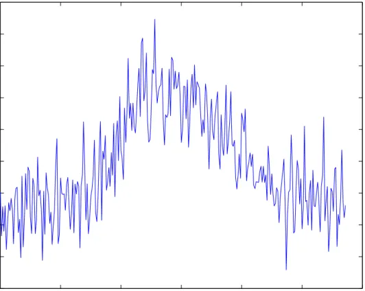
0 50 100 150 200 250 300 0.8 1 1.2 1.4 1.6 1.8 2 2.2 2.4 2.6x 10 8 Time (minutes)

Data rate in bits/sec

Data set II (24 hrs)

Figure 3.1: Time Series plot of Data set II

our prediction with the actual traﬃc. The time series of the data set II is given in Figure 3.1.

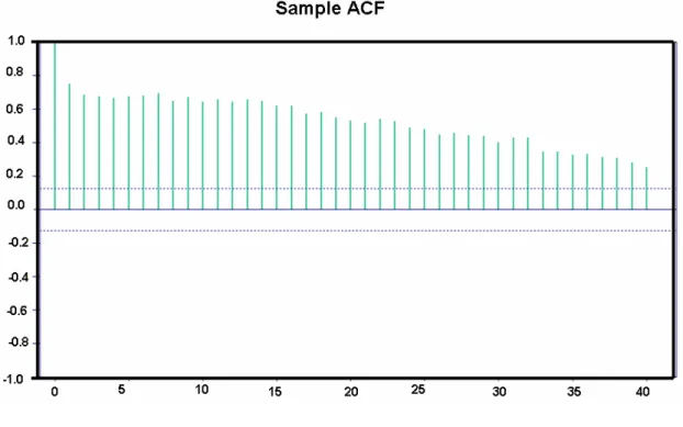
The sample ACF plot of Data set II is given in Figures 3.2. The sample ACF plot sug-gest that the data is non-stationary. In order to remove the non-stationarity and trend in the data, we need to pre-process the data. The aggregated time series is transformed using Box-Cox transformation and diﬀerencing it once. The plot of the transformed data for the data set II is given in Figure 3.3.

(34)

(35)

.60 .40 .20 .00 -.20 -.40 -.60 0 50 100 150 200 250 Series

(36)

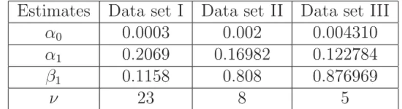
Estimates Data set I Data set II Data set III

α0 0.0003 0.002 0.004310

α1 0.2069 0.16982 0.122784

β1 0.1158 0.808 0.876969

ν 23 8 5

Table 3.1: Parameter Estimates for Data sets I, II and III

3.5.2 Model Identiﬁcation

In order to select the orders p and q we used the modiﬁed Akaike Information Criterion (AICC)33. An exhaustive search is done for various combinations of p and q, using ITSM tool and the model with the minimum AICC is chosen as the best candidate model. The reason for the choice of AICC is because of the fact that metrics like AIC and BIC not only evaluate the ﬁt between values predicted by the model and actual measurements, but also penalize models with larger number of parameters. The best minimum order ofp and q for our model is (1,1).

Once the data is preprocessed, we fitted a GARCH(1,1) model. The unknown parameters of the model, α0, α1, β1 and ν are estimated using the maximum likelihood function. The estimates of all the parameters along with theν-value for data sets I, II and III are listed in Table 3.1. It can be noted that the estimates ofα0, α1, β1 and ν are statistically significant from zero, justifying the GARCH model and its heavy-tailedness of the innovations process. To evaluate the goodness of fit for the GARCH model, we plotted the Q-Q (t-distributed) plot of the GARCH residuals.

3.5.3 Prediction Methodology

For prediction, we have used a one-step prediction recursively to obtain the subsequent values. The ﬁrst 24 hrs of the data set are used as the training part to model the traﬃc; the next 24 hrs are used for performing the forecast and the comparison. In our prediction methodology, we set our forecast step to one. Based on the parameters estimated from the time series using the GARCH model and also on the information obtained from the last

(37)

time instant of the time series data, we proceed to forecast the traffic for the next time instant. We update the traffic data each time the actual traffic is available to us; and this process is recursively performed for the next 24 hrs. This forecasted traffic is compared with the actual traffic data and we compare the performance based on the prediction error. The prediction methodology used is also simple to be performed in real time.

3.6 Results

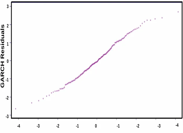
We observed that GARCH model fitted the traffic data very well and this is confirmed by the goodness of fit test which is given by the Q-Q plot with the squared correlation R2 close to 1 as shown in Fig 3.4. Such a well-fitted statistical evidence is a solid empirical foundation for the forecasting and the bandwidth provisioning.

Once the goodness of fit test is done, we did the prediction for the next 24 hrs. In Figure 3.5, we observe that the forecast closely follow the actual traffic. Our forecast technique shows few cases of slight overforecast and rare cases of underforecast, which is a positive point. In order to validate the efficiency of our model, we did a comparative study with other models such as ARIMA(1,1,1), ARCH(1) and ARIMA(1,1,1)-ARCH(1). We used the traffic data to fit all the four models ARIMA, ARCH, ARIMA-ARCH and GARCH and it was observed that GARCH has the best fit. In fact, if there is an under forecasting, this is a concern as there will be underallocation of bandwidth, which can lead to loss of information as a result of the bandwidth restriction. In order to validate the efficiency and complexity of our model, we did a comparative study with other models such as ARIMA, ARCH and ARIMA-ARCH. An analysis of this comparative study is given in the following sections.

3.6.1 Performance

In this section we present comparative forecasting performance results of GARCH with ARIMA, ARCH and ARIMA-ARCH. We used the traﬃc data to ﬁt all the four models

(38)

3 2 1 0 -1 -2 -3 -4 -3 -2 -1 0 -1 -2 -3 -4

Q-Q(t-distribution df = 7.203)GARCH Residuals R^2 = 0.985023

GARCH Residuals

Data Residuals

(39)

0 50 100 150 200 250 300 0.8 1 1.2 1.4 1.6 1.8 2 2.2 2.4 2.6x 10 8 Time (minutes) bps Data set II Predicted Traffic Actual Traffic (a) 0 10 20 30 40 50 60 0.9 1 1.1 1.2 1.3 1.4 1.5 1.6 1.7 1.8x 10 8 Time (minutes) bps Data set II Predicted Traffic Actual Traffic ((b)

Figure 3.5: Predicted Traﬃc for Data set II (a) 24 hrs interval (5 min aggregation) (b) Enlarged view of (a) from interval 0-60

(40)

1.00 .80 .60 .40 .20 .00 -.20 -.40 -.60 -.80 1.00 0 5 10 15 20 25 30 35 40 1.00 .80 .60 .40 .20 .00 -.20 -.40 -.60 -.80 -1.00 0 5 10 15 20 25 30 35 40

Residual ACF: Absolute values Residual ACF: Squares

Figure 3.6: ACF plot of absolute value and squares of ARIMA model for data set I

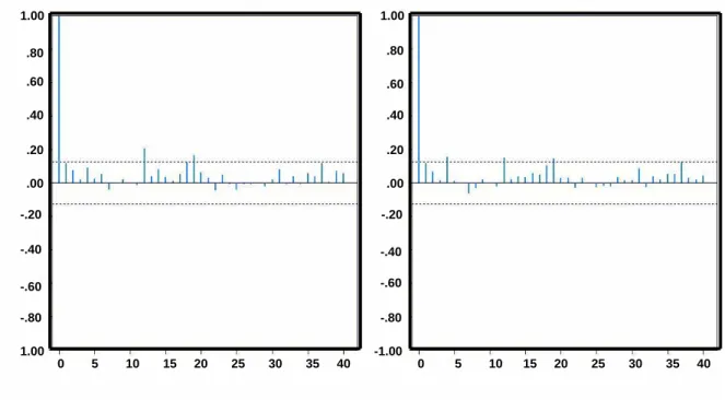
ARIMA, ARCH, ARIMA-ARCH and GARCH and observe how well these fitted models work. To check the goodness of fit for these models we observed the sample ACF/PACF of the residuals of the fitted model.

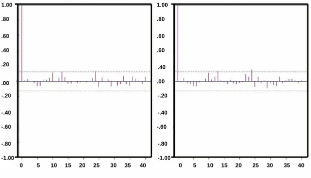
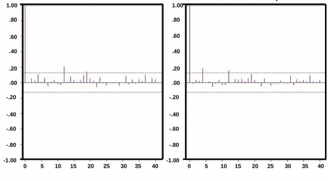
As we can observe from the Figures 3.6, 3.7 and 3.8, the residuals of ARIMA, ARCH and ARIMA-ARCH for all the three data sets are significantly different from zero, while in the case of GARCH as in Figure 3.9, the sample ACF have residual significantly close to zero. These results clearly shows the good performance capability of our model. Our model is able to fit the traffic data accurately as compared to the other model. To further check on the performance of our model we did a more elaborate comparative study on the forecasting behavior of our model and ARIMA-ARCH. In Fig 3.10 (b), we observe that

(41)

1.00 .80 .60 .40 .20 .00 -.20 -.40 -.60 -.80 -1.00 1.00 .80 .60 .60 .40 .00 -.20 -.40 -.60 -.80 -1.00 0 5 10 15 20 25 30 35 40 0 5 10 15 20 25 30 35 40

ARCH residual ACF: Absolute values ARCH residual ACF: Squares

Figure 3.7: ACF plot of absolute value and squares of residuals of ARCH model for data

(42)

1.00 .80 .60 .40 .20 .00 -.20 -.40 -.60 -.80 -1.00 1.00 .80 .60 .40 .20 .00 -.20 -.40 -.60 -.80 -1.00 0 5 10 15 20 25 30 35 40 0 5 10 15 20 25 30 35 40

Arima-Arch residuals ACF: Abs values Arima-Arch residuals: Squares

(43)

1.00 .80 .60 .40 .20 .00 -.20 -40 -.60 -.80 -1.00 1.00 .80 .60 .40 .20 .00 -.20 -.40 -.60 -.80 -1.00 0 5 10 15 20 25 30 35 40 0 5 10 15 20 25 30 35 40

GARCH Residuals ACF: Abs Values _{GARCH Residuals ACF: Squares}

(44)

the forecasting behavior of ARIMA-ARCH though closely follows that of the actual traffic, it underforecast the actual traffic in some cases. This is disadvantageous when it comes to bandwidth allocation as this can lead to a stringent bandwidth allocation. Our model neither underforecast nor excessively overforecast, which is just appropriate for a proper bandwidth allocation. But in the case of GARCH in almost all the three data sets that we studied, the forecasting is a little over the actual traffic. Our model neither under forecast nor excessively over forecast, which is just appropriate for a proper bandwidth allocation. We also did a more elaborative study to compare the performance quantitatively considering the accuracy of the prediction and the complexity of parameter estimation. To measure the accuracy, we have used the following metrics:

• GARCH Forecast Error EG=

N

i=1(Xi−XiG)2

N

i=1Xi2

• ARCH Forecast Error E_A=

N

i=1(Xi−XiA)2

N

i=1Xi2

where Xi−X_iG is the prediction error for GARCH model and Xi−X_iA is the prediction error for ARCH model.

To measure the complexity we have considered the number of parameters to be estimated in each model.

3.6.2 Evaluation

In this section we evaluate the performance and complexity of our model using the above metrics. For each data set, we use the first 24 hours data for developing the time series model and consider the next 24 hrs for evaluating the effectiveness of our approach. To check the performance on a longer time interval, we applied the forecasting algorithm for a period of 7 days. As can be seen from Figure 3.11, we observed that the predicted traffic closely follows the actual traffic. This is a very good indication that GARCH model is able to perform well even for longer time intervals.

To evaluate the forecast accuracy of GARCH model, we did a comparative study with the existing model ARIMA-ARCH. As seen from Table 3.2, we observed that the forecast

(45)

0 50 100 150 200 250 300 0.8 1 1.2 1.4 1.6 1.8 2 2.2 2.4 2.6 2.8x 10 8 Time (minutes) bps Data set II GARCH Actual Traffic ARIMA−ARCH (a) 60 80 100 120 140 160 180 0.8 1 1.2 1.4 1.6 1.8 2 2.2 2.4 2.6 2.8x 10 8 Time (minutes) bps Data set II GARCH Actual Traffic ARIMA−ARCH ((b)

Figure 3.10: Forecasting analysis of GARCH and ARIMA-ARCH (a) 24 hrs interval (5

min aggregation) (b) Enlarged view of (a) from interval 60-180

error of GARCH model is signiﬁcantly smaller than ARIMA-ARCH model, which clearly states the forecast eﬃciency of GARCH.

(46)

Error Data set I Data set II Data set III Garch 7.2652 x 10−13 3.3393 x 10−12 1.759 x 10−10 ARCH 1.1818 x 10−4 1.8501 x 10−5 2.0413 x 10−4

Table 3.2: Prediction errors of GARCH and ARCH for Data sets I, II and III

0 200 400 600 800 1000 1200 1400 1600 1800 0 0.5 1 1.5 2 2.5 3x 10 8 time(minutes) bps

Data set II (7days)

predicted traffic actual traffic

(47)

parameters to be estimated, since the selected GARCH model has order (1,1), while the selected ARIMA-ARCH model has order (1,1,1).

3.7 Conclusion

In our study, we introduced GARCH - a non-linear time series model, which is capable of capturing specific characteristics of Internet traffic data which the traditional linear time series failed to accommodate. Our model can capture the bursty nature of Internet traffic with its variable variance. Statistically, if the traffic has a bursty behavior, this means that it has a variance changing with time. The GARCH model is a non-linear time series model which can capture the conditional variance effectively, because of its dependence on variance at every time instant. Our model is able to forecast aggregated traffic but further investigation need to be conducted on a less aggregated traffic. Since we could forecast the traffic data successfully using a simple prediction methodology based on our GARCH model, we also intend to develop a dynamic bandwidth allocation algorithm as a future work.

(48)

Chapter 4 Conclusion and Future Work

The objective of this thesis is to come up with a model and a forecasting algorithm which can best represent the Internet traffic data and its characteristics. We developed a model using non linear time series model, Generalized Autoregressive Conditional Heteroskedasticity (GARCH) model of order (1,1). GARCH model fitted the data very well and the bursty nature of the Internet traffic is also taken care of by the conditional variance of GARCH model. Our goodness of fit test is able to determine that the model fitted the data well.

We have used a simple forecasting algorithm based on model used. The comparision with the actual traffic clearly showed that the forecast algorithm is accurate. The predicted traffic clearly followed the actual traffic. From the comparision with other models we can conclude that GARCH has better performance. Since our model is of order (1,1), it is less complex compared to other model. So from performance and complexity point of view GARCH is found to be a good model from our study. However, the forecast algorithm is developed based on the model fitting of aggregated traffic and further investigation need to be carried out on a less aggregated traffic.

We see dynamic bandwidth provisioning scheme as a potential future work. Based on the GARCH model and the forecasting algorithm developed, we can develop a dynamic bandwidth provisioning methodology.

(49)

Bibliography

[1] W. E. Leland, M. S. Taqqu, W. Willinger, and D. V. Wilson, On the Self-Similar Nature of Ethernet Traﬃc, in Proceedings of ACM SIGCOMM’ 93, pages 183–193, 1993.

[2] T. Karagiannis, M. Molle, and M. Faloutsos, A Nonstationary Poisson View of Internet Traﬃc, in IEEE INFOCOM 2004, volume 3, pages 1558–1569, Hong Kong, 2004.

[3] A. Feldmann, A.C.Gilbert, W. Willinger, and T. Kurtz, The changing nature of network traﬃc: scaling phenomena, in ACM SIGCOMM Computer Communication Review, volume 28, pages 5–39, 1998.

[4] V. Paxson and S. Floyd, Wide-Area traﬃc: The Failure of Poisson Modeling, in IEEE/ACM Transactions on Networking, volume 3, pages 226–244, 1995.

[5] W. E. L. M. S. Taqqu, W. Willinger, and D. V. Wilson, On the Self-Similar Nature of Ethernet Traﬃc(Extended Version), in IEEE/ACM Transactions on Networking, volume 2, pages 1–15, 1994.

[6] T. Kariagianis, M. Molle, and M. Faloutsos, Long Range Dependence - Ten Years of Internet Traﬃc Modeling, in IEEE Internet Computing, 2004.

[7] M. Crovella and A. Bestavros, Self Similarity in World Wide Web Traﬃc: Evidence and Possible Causes, in IEEE/ACM Transactions on Networking, volume 5, pages 835–846, 1997.

[8] M. Zukerman, T. Neame, and R. Addie, Internet Traﬃc Modeling and Future Tech-nology Implications, in IEEE INFOCOM 2003, volume 1, pages 587– 596, 2003.

(50)

[9] A. Sang and S. LiX, A predictability analysis of network traﬃc, in INFOCOM 2000, volume 1, pages 342 – 351, 2000.

[10] S. Basu, A. Mukherjee, and S. Klivansky, Time Series Models for Internet Traﬃc, in IEEE INFOCOM96, California, USA, 1996.

[11] M. Corradi, R. G. Garroppo, s. Giordano, and M. Pagano, Analysis of f-ARIMA processes in the modeling of broadband traﬃc, in ICC’01, volume 3, pages 964–968, 2001.

[12] Y. Shu, M. Yu, J. Liu, O. Yang, and H. Feng, Wireless Traﬃc Modeling and Prediction using Seasonal ARIMA models, in IEICE Transactions on Communications, volume E88-B, pages 3992– 3999, 2005.

[13] C. You and K. Chandra, Time Series Models for Internet Data Traﬃc, in 24th Conf. on Local Computer Networks, LCN’99, 1999.

[14] B. Krithikaivasan, Y. Zeng, K. Deka, and D. Medhi, ARCH-based Traﬃc Forecasting and Dynamic Bandwidth Provisioning for Periodically Measured Nonstationary Traﬃc, in IEEE/ACM Transactions on Networking, volume 10, pages 870–883, 2006.

[15] B. Zhou, D. He, and Z. Shun, Traﬃc Modeling and Perdiction using ARIMA/GARCH Model, inSymposium on Modeling ans Simulation tool for emerging telecommunications networks: needs, trends, challenges and solutions, Meunchen, Germany, 2005.

[16] C. Barakat, P. Thiran, G.Iannaccone, C.Diot, and P. OwezarskiV, A ﬂow-based model for internet backbone traﬃc, inProceedings of the 2nd ACM SIGCOMM Workshop on Internet measurment, pages 35–47, 2002.

[17] B. Chen, S. Peng, and K. Wang, Traﬃc Modeling, Prediction, and Congestion Control for High-Speed Networks: A Fuzzy AR Approach., in IEEE/ACM Transactions on Fuzzy Systems, volume 8, 2000.

(51)

[18] A. D. Doulamis, N. D. Doulamis, and S. D. Kollias, An Adaptable Neural Net-work Model for Recursive Nonlinear Traﬃc Prediction and Modeling of MPEG Video Sources, in IEEE Transactions on Neural Networks, volume 14, pages 150–166, 2003.

[19] X. Tian, H. Wu, and C. Ji, A uniﬁed framework for understanding network traﬃc using independent wavelet models, in INFOCOM 2002, volume 1, pages 446–454, 2002.

[20] C. Bruni, P. Andrea, U. Mocci, and C. Scoglio, Optimal Capacity Management of Virtual Paths in ATM Networks, in GLOBECOM 94, pages 207–211, 1994.

[21] S. Ohta and K. Sato, Dynamic Bandwidth Control of the Virtual Path in an Asyn-chronous Transfer Mode Network, in IEEE/ACM Transactions on Communications, volume 40, pages 1239–1247, 1992.

[22] A. Orda, G. Paciﬁci, and D. Pendarakis, An Adaptive virtual Path Allocation Policy for Broadband Networks, in IEEE INFOCOM 96, pages 329–336, 1996.

[23] Y. Afek, M. Cohen, E. Haalman, and Y. Mansour, Dynamic bandwidth allocation policies, in IEEE INFOCOM96, pages 880–887, 1996.

[24] K. Papagiannaki, N. Taft, Z. Zhang, and C. Diot, Long-Term Forecasting of Internet Backnone Traﬃc: Observations and Initial Models, in IEEE INFOCOM 03, pages 1178–1788, 2003.

[25] B. Krishnamurthy, S. Sen, Y. Zhang, and Y. Chen, Sketch-based Change detection: Methods, Evaluation, and Applications, inInternet Measurement Conference(IMC 03), Miami, USA, 2003.

[26] J. Jiang and S. Papavassiliou, Detecting Network Attacks in the Internet via Statistical Network Traﬃc Normality Prediction., in Journal of Network and Systems Manage-ment, volume 12, pages 51–72, 2004.

(52)

[27] N. Feamster, L. Gao, and J. Rexford, CABO: Concurrent Architectures are Better Than One, in FIND Project, 2006.

[28] B. Krithikaivasan, K. Deka, and D. Medhi, Adaptive Bandwidth Provisioning based on Discrete Temporal Network Measurements, in IEEE INFOCOM04, pages 1786–1796, Hong Kong, China, 2004.

[29] P. Chemouil and J. Filipiak, Modeling and Prediction of Traﬃc Fluctuations in Tele-phone networks., in IEEE/ACM Transactions on Communications, volume 35, pages 931–941, 1987.

[30] N. K. Groschwitz and G. C. Polyzos, A Times Series Model of Long-Term NSFNET Backbone Traﬃc, in ICC 94, pages 1400–1404, 1994.

[31] P. Cortez, M. Rio, M. Rocha, and P. Sousa, Internet Traﬃc Forecasting using Neural Networks, in IEEE IJCNN, 2006, pages 2635–2642, 2006.

[32] http://abilene.internet2.edu/.

[33] P. J. Brockwell and R. A. Davis, Introduction to Time Series and Forecasting, Springer, New York, 2002.

[34] J. Beran, Statistics for Long-Memory Processes, Chapman and Hall, 1994.

Internet traffic modeling and forecasting using non-linear time series model GARCH