DIFFERENTIATION MATRICES FOR MEROMORPHIC FUNCTIONS

(1)

DIFFERENTIATION MATRICES FOR MEROMORPHIC FUNCTIONS

RAFAEL G. CAMPOS AND CLAUDIO MENESES

Abstract. A procedure for obtaining differentiation matrices is extended straightforwardly to yield new differentiation matrices useful for derivatives of complex rational functions. Such matrices can be used to obtain numer-ical solutions of some singular differential problems defined in the complex domain. The potential use of these matrices is illustrated with the case of elliptic functions.

1. Introduction

In a series of papers ([4]-[6] and references therein), a Galerkin-type method has been used to solve boundary value problems and to find limit-cycles of nonautonomous dynamical systems. The method is based on the discretization of the differential problem by using differentiation matrices that are projec-tions of the derivative in spaces of algebraic polynomials or trigonometric poly-nomials. This kind of matrices arise naturally in the context of interpolation of functions and yield exact values for the derivative of polynomial functions at certain points selected as nodes. The class of functions that defines the do-main of the differential operator determines the kind of differentiation matrix to be used. Thus, to get a discrete form of an operator acting on real functions that drop off rapidly to zero at large distances, we can use the skew-symmetric differentiation matrix (1.1) Djk =          0, i=j, (−1)j+k xj−xk , i6=j,

constructed with theN zerosxj of the Hermite polynomialHN(x) as lattice points1_{. On the other hand, to get a discrete form of an operator acting on} periodic functions [7], the differentiation matrix

(1.2) Djk=          0, j=k, (−1)j+k 2 sin(xj−xk) 2 , j6=k,

2000Mathematics Subject Classification: 65D25, 41A05, 42A15.

Keywords and phrases: numerical differentiation, complex interpolation, meromorphic func-tions, trigonometric polynomials.

1_{Equation (1.1) gives an asymptotic expression for}_D x. 121

(2)

should be used. In this case the lattice points can be chosen as theN equidis-tant points

(1.3) xj=−π+ 2πj/N, j= 1,2,· · ·, N.

Discrete forms of multidimensional differential operators can be obtained by using direct products of suitable one-dimensional differentiation matrices (see [5] for instance).

Other approaches to obtaining differentiation matrices can be found in [10]. The purpose of this paper is to use the complex Hermite interpolation for-mula to find new differentiation matrices on the complex domain that produce an exact formula for the derivatives of complex rational functions and that can be used to approximate the solution of a singular differential equation in the complex domain. As examples, the derivatives of meromorphic two-periodic functions such as Jacobi elliptic functions and Weierstrass elliptic functions will be used to show the potential of this technique.

2. Interpolatory differentiation matrices

In order to illustrate the procedure for generating differentiation matrices, an already known matrix [3], which gives the derivative of algebraic polyno-mials of the complex variablezis obtained by using the Hermite interpolation formula.

(2.1) Algebraic polynomials. Letf(z) be an analytic function on a domain

Gcontaining a closed rectifiable Jordan curveγand letzkbeNdifferent points ofI(γ) defining the polynomial

ω(z) = N

Y

k=1

(z−zk).

Then the unique polynomial p(z) interpolating f(z) associated to the set of pointszkis given by ([8], [9]) (2.1.1) p(z) = 1 2πi Z γ f(ζ) ω(ζ) ω(ζ)−ω(z) ζ−z dζ.

The residual functionR(z) =f(z)−p(z),z∈I(γ) vanishes atzk, yielding that f(zk) =p(zk). To see this, writeR(z) as

(2.1.2) R(z) =ω(z) 2πi Z γ f(ζ) (ζ−z)ω(ζ)dζ.

Since the integral of the right-hand side of this equation represents an analytic function onI(γ) we have thatR(zk) = 0.

To obtain the form ofp(z), the integral in equation (2.1.1) can be calculated by the residue theorem. Sinceω(ζ)−ω(z) is divisible byζ−z, the integrand has simple poles only atz1, . . . , zN. Thus the residue theorem yields the well-known Lagrange interpolation formula

(2.1.3) p(z) = N X j=1 f(zj) QN k6=j(z−zk) QN k6=j(zj−zk) , z∈G.

(3)

The differentiation matrixDassociated to this formula can be obtained if the derivative of (2.1.3) is evaluated atziand written as

(2.1.4) dp(zi) dz = N X j=1 Dijf(zj). Since d dz   N Y k6=j (z−zk)/ N Y k6=j (zj−zk)   z=zi =                  QN k6=i,j(zi−zk) QN k6=j(zj−zk) , i6=j, N X k6=i 1 (zi−zk) , i=j,

we get that the differentiation matrix for algebraic polynomials is given by

(2.1.5) Dij=                N X k6=i 1 (zi−zk) , i=j, ω0₍_z i) (zi−zj)ω0(zj) , i6=j.

Iff(z) is a polynomial of degree at mostN−1,f(z) is given identically byp(z) and therefore formula (2.1.4) gives the exact derivative off(z). Sincef0₍_z_{) is} another polynomial in this class, the derivatives of higher order can be obtained by applying successively the matrixDto the vector of valuesf(zj), i.e., (2.1.6) f(n) =Dnf, n= 0,1,2, . . . .

Here, f(n) _{is the vector whose entries are} _dn_f₍_z

i)/dzn, Dn is the nth power ofD andf is just the vector whose entries aref(zi). The functional form of f(n)₍_z_{) can be obtained through an interpolation of the values yielded by (2.1.6).} Since any set ofNdifferent complex numbers belonging toGyields the same polynomialf(z), this result is independent of the pointszk. On the other hand, iff(z) is not a polynomial of degree at mostN−1 a residual vector should be added to the right-hand side of (2.1.4) to getf0₍_z

i). However, such a formula yields an good approximation tof0₍_z

i) if the absolute value of theM-th term of the Taylor series off(z) goes to zero rapidly asM is increased.

(2.2) Trigonometric polynomials. The preceding arguments can be modi-fied to consider the interpolation of periodic functions in terms of trigonometric polynomials. Letf(z) be a one-periodic analytic function with period 2πand letGbe a domain of the open strip−π <<z < π,−∞<=z <∞, containing a closed rectifiable Jordan curveγ.

Since any trigonometric polynomialτ(z) =a0+Pmk=1(akcoskz+bksinkz) of degree at mostmcan be written in the form ˜τ(s) =s−m_q₍_s_{) under the the} mappings=ϕ(z) =eiz_where_q₍_s_{) is a polynomial of degree at most 2}_m_in_s_, we need to take an odd numberN = 2m+ 1 of different pointssk ∈ϕ(I(γ)), i.e, 2m+ 1 different pointszk∈I(γ), to yield an exact interpolation formula in

(4)

the case in whichf(z) is a trigonometric polynomial of degree at mostm. This fact can be shown as follows.

Let us takeN= 2m+ 1. The set of pointssk,k= 1,2, . . . , Ndefine the poly-nomial ˜ω(s) =QN

k=1(s−sk). The interpolant function ˜p(s) to ˜f(s) =f(ϕ−1(s)) corresponding to the set ofNpointsskis given by

(2.2.1) p˜(s) = s −m 2πi Z ˜ γ ˜ f(ζ) ˜ ω(ζ) sm_ω_˜₍_ζ₎₋_ζm_ω_˜₍_s₎ ζ−s dζ,

where ˜γ=ϕ(γ). Since [sm_ω_˜₍_ζ₎₋_ζm_ω_˜₍_s_)]_/₍_ζ₋_s_{) is a polynomial in}_s_{of degree} N−1 = 2m, ˜p(s) has the required forms−m_q₍_s_{), where}_q₍_s_{) is a polynomial of} degree at most 2m, to represent a trigonometric polynomialτ(z).

To show that ˜f(sk) = ˜p(sk), let us consider the residual function ˜R(s) = ˜ f(s)−p˜(s) which is now ˜ R(s) = 1 2πi ˜ ω(s) sm Z ˜ γ ˜ f(ζ)ζm (ζ−s) ˜ω(ζ)dζ.

By definition, ˜G = ϕ(G) does not contains points sk(mod 2π) other than sk; therefore, the integral of the right-hand side of this equation represents an analytic function inI( ˜γ) and we have that ˜R(sk) = 0.

Since sm_ω_˜₍_ζ₎₋_ζm_ω_˜₍_s_{) is divisible by}_ζ₋_s_{, the poles of the integrand are} simple and located atsk. The residue theorem yields now

(2.2.2) p˜(s) = N X j=1 ˜ f(sj) s_j s m Q N k6=j(s−sk) QN k6=j(sj−sk) , s∈G˜

and the trigonometric polynomial of degreem= (N−1)/2 that interpolates

f(z) is (2.2.3) p(z) = N X j=1 f(zj)ei(N−1)(zj−z)/2 QN k6=j(eiz−eizk) QN k6=j(eizj−eizk) , z∈G. Since ei(N−1)(zj−z)/2 QN k6=j(eiz−eizk) QN k6=j(eizj−eizk) = QN k6=jsin z−zk 2 QN k6=jsin _z j−zk 2 , we obtain from (2.2.3) the Gauss interpolation formula

(2.2.4) p(z) = N X j=1 f(zj) QN k6=jsin z−zk 2 QN k6=jsin _z j−zk 2 , N = 2m+ 1, z∈G.

By writing the derivative of this formula in the form given by (2.1.4) we can obtain the differentiation matrix for trigonometric polynomials. Thus the

(5)

matrixDwhose entries are given by (2.2.5) Dij =                      1 2 N X k6=j cot _z j−zk 2 , i=j, 1 2csc zi−zj 2 QN k6=isin( zi−zk 2 ) QN k6=jsin( zj−zk 2 ) , i6=j,

in terms ofN = 2m+ 1 different pointszk ∈G, is a projection ofd/dzin the subspace of trigonometric polynomials of degree at most (N−1)/2. Therefore, iff(z) belongs to this space,p(z)≡f(z), andf(n)₍_z_{) satisfies again an equation} like (2.1.6) but in this caseDn _{is the}_n_{th power of (2.2.5). The form of}_f(n)₍_z₎ can be obtained from the set of valuesf(n)₍_z

i) through an interpolation. For a general one-periodic analytic function with period 2πa residual vector should be added to (2.2.4).

It is worth to notice that in the case in which the set of pointszk are real numbers, the matrix (2.2.5) becomes the matrix used previously in [6], [7]. However, if the points lay on a straight line which is parallel to the imaginary axis,Dtakes the form

Dij =                      −i 2 N X k6=i coth _y i−yk 2 , i=j, −i 2csch _y i−yj 2 QN k6=jsinh( yi−yk 2 ) QN k6=isinh( yj−yk 2 ) , i6=j,

whereyk==zk, at the same time that the polynomial to differentiate becomes a linear combination of real hyperbolic functions.

(2.3) Rational functions. Equation (2.2.1) suggests the form of a interpolant rational function in the case in whichf(z) is a meromorphic function.

LetGbe a domain that contains a closed rectifiable Jordan curveγand let

f(z) be a meromorphic function with only one pole atz =α 6∈ Gof orderm. Let us chooseNdifferent pointszkofI(γ) and construct the polynomialω(z) =

QN

k=1(z−zk). Thus the rational function interpolating f(z) corresponding to the set of pointszkis given by

(2.3.1) p(z) =(z−α) −m 2πi Z γ f(ζ) ω(ζ) (z−α)m_ω₍_ζ₎₋₍_ζ₋_α₎m_ω₍_z₎ ζ−z dζ.

This can be shown by the same arguments used in the previous case. Again, (z−α)m_ω₍_ζ₎₋₍_ζ₋_α₎m_ω₍_z_{) is divisible by}_ζ_−z_{. Let}_Km N(z, ζ) be such a quotient, i.e., K_Nm(z, ζ) = (z−α) m_ω₍_ζ₎₋₍_ζ₋_α₎m_ω₍_z₎ ζ−z . SinceKm

N(z, ζ) is a polynomial of degreeN−1 inz,p(z) is a rational function of formq(z)/(z−α)m_{that interpolates to}_f₍_z_{) at}_z

(6)

of degree at mostN−1. The residual function R(z) = 1 2πi ω(z) (z−α)m Z γ f(ζ)(ζ−α)m (ζ−z)ω(ζ) dζ.

vanish atzk because the integral is an analytic function inI(γ) andα 6∈ G. Therefore,p(zk) =f(zk). The residue theorem yields now

(2.3.2) p(z) = N X j=1 f(zj) _z j−α z−α m QN k6=j(z−zk) QN k6=j(zj−zk) , z∈G.

The derivative of this equation atzican be written in the form (2.1.4) where we have now (2.3.3) Dij =                N X k6=i 1 (zi−zk) − m zi−α , i=j, (zj−α)m/(zi−α)m zi−zj ω0₍_z i) ω0₍_z j) , i6=j.

Obviously, iff(z) is a rational function of the formq(z)/(z−α)m whereq(z) is a polynomial of degree at mostN−1,f(z)≡p(z) and formula (2.1.4) becomes

(2.3.4) df(zi) dz = N X j=1 Dijf(zj).

However, the powers ofDdo not give the derivatives of higher order as in the previous cases sincef0₍_z_{) does not has the required form: it has a pole of order}

m+ 1 atz=α. Despite this, it is possible to obtain the value off(n)₍_z_{) at}_z kby using the matrix

(2.3.5) Dn(m) =Dm+n−1Dm+n−2· · ·Dm.

Each matrixDkis defined by (2.3.3) where the parameterm, defining the order of the pole, is substituted by each value of the indexk. Thus, it should be clear that iff(z) has the form given above, (2.1.6) becomes

(2.3.6) f(n)=Dn(m)f, n= 0,1,2, . . . .

This equation can be generalized to the case in whichf(z) is a rational function of form

(2.3.7) f(z) =

PM

k=0akzk

(z−α1)m1(z−α₂)m2· · ·(z−α_r)mr

whereαl6∈G,l= 1,2,· · ·, r. A straightforward calculation gives the general-ized form of (2.3.6)

(2.3.8) f(n)=Dn(m1, m2, . . . , mr)f, n= 0,1,2, . . . , where nowDn(m1, m2, . . . , mr) stands for the ordered matrix product (2.3.9) Dn(m1, m2, . . . , mr) =

0

Y

k=n−1

(7)

andDµ1,µ2,...,µris the matrix whose entries are given by (2.3.10) (Dµ1,µ2,...,µr)ij=                  N X k6=i 1 (zi−zk) − r X k=1 µk zi−αk , i=j, 1 zi−zj ω0₍_z i) ω0₍_z j) r Y k=1 _z j−αk zi−αk µk , i6=j.

It should be noticed that (2.3.8) is an exact formula wheneverN ≥M+nr−1, where M is the degree of the polynomial in the numerator of (2.3.7). The reason is that after each differentiation the numerator of the derivatives of

f(z) is a polynomial whose degree grows byr. If the functionf(z) to differ-entiate has poles at α1, . . . , αr of orders n1, . . . , nr instead m1, . . . , mr, with n1 < m1, . . . , nr < mr, formula (2.3.8) is still exact wheneverN ≥M +nr− 1 +Pr

k=1(mk −nk). The reason for this is that in such a case f(z) can be writen in the form (2.3.7) where the numerator is now a polynomial of degree

M+Pr

k=1(mk−nk). Obviously, in this case is much better to use the differ-entiation matrix Dn(n1, n2, . . . , nr) instead Dn(m1, m2, . . . , mr) for numerical purposes.

3. Applications

As stated before, the numerical solution of differential problems can be ac-complished by the use of differentiation matrices, and in the case of a differ-ential problem in the complex domain, the differentiation matrices introduced in this paper may be useful. To illustrate the potential of their use, we choose two meromorphic cases which are important in applications: Jacobi elliptic functions and Weierstrass elliptic functions. In both cases it is possible to es-tablish the numerical convergence of the results since the derivatives of these functions are known. We also obtain approximate solutions of a differential equation with a regular singularity atz= 0. Before beginning these examples is convenient to alert the reader to the fact that the numerical implementation of the matrices for rational functions given above may need a high-precision code: in most cases, the usual 16-digit precision is not enough to obtain accu-rate results.

(3.1) A rational function. Let us consider the function

(3.1.1) f(z) =z

7₊_z_{+ 1} z10 .

According to the results of the last section, to obtain the exact value of then-th derivative of (3.1.1), [cf. Eq. (2.3.6)], it is necessary to chooseN >7 different pointszk6= 0 in the complex plane to build the matrix (2.3.5) where obviously, α= 0 andm= 10.

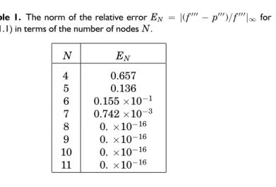
As an example, let us take the third derivative of (3.1.1). Table 3.1 shows the max-norm of the vector whose entries are

|[f(3)₍_z

j)−PNk=1(D3(10))jkf(zk)]/f(3)(zj)|(the relative error) in terms ofN. The nodes were chosen to be as evenly spaced on the rayz= (1 +i)t, 1/2< t≤1, i.e.,zk = (1 +i)(1 +k/N)/2,k = 1, . . . , N, and the computations were made

(8)

Table 1. The norm of the relative errorEN = |(f000−p000)/f000|∞ for

(3.1.1) in terms of the number of nodesN.

N EN 4 0.657 5 0.136 6 0.155×10−1 7 0.742×10−3 8 0. ×10−16 9 0. ×10−16 10 0. ×10−16 11 0. ×10−16

with the standard 16-digit precision. As it can be seen from Table 3.1, the error vanishes for values ofNgreater than 7, as expected.

(3.2) Elliptic functions. As is known, an elliptic function is a doubly periodic function which is analytic except at poles [2]-[1] and one of the two simplest cases of elliptic functions corresponds to Jacobi’s functions; the other corre-sponds to Weierstrass’℘-function.

The differentiation matrices given above do not apply to functions like these; however, it is possible to build a matrix which is expected to provide approx-imate values off(n)₍_z

k) along straight lines inside the fundamental paralelo-grams and near the poles. Since an elliptic functionf(z) becomes a one-periodic function ifzis constrained to move along a straight line defined by one of the periods, such a matrix can be constructed by using trigonometric polynomials divided by an algebraic polynomial with zeros of suitable orders taken at the poles off(z). This procedure is equivalent to taking apart the matrix (2.3.10) and incorporating only the singular terms in (2.2.5) to yield the new matrices (3.2.1) D˜n(m1, m2, . . . , mr) = 0 Y k=n−1 ˜ Dm1+k,m2+k,...,mr+k, where (3.2.2) ( ˜Dµ1,µ2,...,µr)ij =                  N X k6=i cot zj−zk 2 − r X k=1 µk zi−αk , i=j, 1 2csc zi−zj 2 N Y k6=i sin(zi−zk)/2 sin(zj−zk)/2 r Y k=1 zj−αk zi−αk µk , i6=j.

To test the numerical performance of this matrix we choose two numerical examples. The first one corresponds to Jacobi’s functionf(z) = sn(z|1

(9)

has two periods 4Kand 2iK0_{and two simple poles at}_iK0_{and 2}_K₊_iK0_{, where} K= Z π/2 0 dθ q 1−(sin2θ)/2 , K0 =K ≈1.854.

Therefore, to build the differentiation matrix we take 2π-periodic trigonomet-ric polynomials,r = 2,µ1 =µ2 = 1,α1=iK0, andα2= 2K+iK0 in (3.2.2), and to measure the approximation off0(zj) byp0(zj) =PNk=1( ˜D1(1,1))jkf(zk) we use the max norm. Here, f0₍_z_{) = cn(}_z|1

2) dn(z| 1

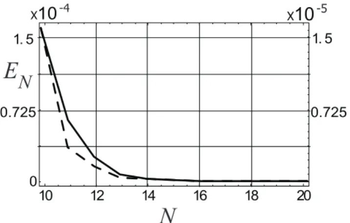
2). The results are dis-played in Figure 1, where the max-norm of the errorf0₍_z

j)−p0(zj) is plotted against the number of nodes showing numerical convergence. The number of digits of precision used in the calculations is 16 and the nodes are chosen to be evenly spaced on the rayz= (2 +i)t, 1/2< t≤1, i.e.,zk= (2 +i)(1 +k/N)/2, k = 1, . . . , N. The norm of the error is 1.6×10−4_for_N _{= 10 and 1}_.₀_×₁₀−8 forN= 20.

Our second example is the Weierstrass℘-function, which has a double pole at the origin and two periodsω1andω2. The derivative of℘(z) satisfies

(℘0(z))2= 4(℘(z))3−g2℘(z)−g3,

whereg2andg3are the elliptic invariants which are related to bothω1andω2 [1].

To approximate the first derivative of℘(z) at the nodes, we need to take

n = 1 and r = 1 in (3.2.1) and µ1 = 2 and α1 = 0 in (3.2.2). The precision of the calculations, the nodes, and the kind of trigonometric polynomials used to construct the differentiation matrix are the same as above. The numerical results are displayed in Figure 1 and show again numerical convergence with a small number of nodes. ForN = 10 the norm of the error is 1.5×10−5_and 1.0×10−8_for_N _{= 20.}

Figure 1: The norm of the errorEN = |f0−p0|∞against the number of nodes for the

Jacobian elliptic function (solid line) and Weierstrass’℘-function (broken line). The vertical axes are scaled according to Jacobi’s case (the left-hand axis) or Weierstrass’ case (the right-hand axis).

(10)

(3.3) Krummer’s equation. As a final example, we consider the Krummer differential equation, written as an eigenvalue problem

(3.3.1) zd

2_f₍_z₎

dz2 + (b−z) df(z)

dz =af(z),

which has a regular singularity atz = 0 and an irregular singularity at∞. As is well known, the single-valued solution of this equation is the confluent hypergeometric functionM(a, b, z) =1F1(a, b, z). Since this function can be ap-proximated by algebraic polynomials forb6=−n(na positive integer), we can obtain approximate solutions of this differential equation by using the differ-entiation matrixDgiven by (2.2.5) to approximate the derivative ofM(a, b, z) and solving theN-dimensional eigenvalue problem

(3.3.2) Lfλ=λfλ, L=ZD2+ (b1N−Z)D

whereZis a diagonal matrix whose nonzero elements are the nodesz1, . . . , zN, bis a complex number (b6=−n), 1N is the identity matrix of dimensionNand the eigenvalueλis the value ofaat whichM(a, b, zk) is to be approximated by (fλ)k. Let us denote byMa the vector whosekth component isM(a, b, zk). Since thenth coefficient of the power series ofM(a, b, z) is given by

a(a+ 1)(a+ 2). . .(a+n−1)

b(b+ 1)(b+ 2). . .(b+n−1)n!,

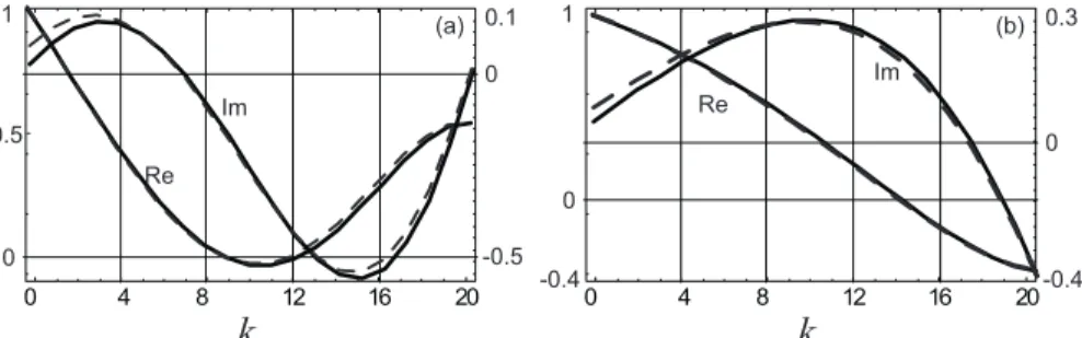
the best approximation obtained for a given set of parametersb,N,zk, is given by the eigenvector fλ (λ = a) corresponding to the eigenvalue with lowest absolute valueλm. To construct the matrixLin (3.3.2) we chooseN = 21 and zk= 5(1 +i)k/N,k= 1, . . . N. Forbwe take the casesb= 5/2 andb= 3 + 2i. In order to compare the approximate and exact results, we normalize both vectorsMλmandfλmwith the max-norm. The calculations were made with 16 digits of precision and the results are displayed in Fig. 2. The absolute errror

kMλm−fλmk0is 0.0675659 forb= 5/2 and 0.0426948 forb= 3 + 2i.

Figure 2: Normalized real (Re) and imaginary (Im) parts offλmplotted versus their index

(solid lines). Case (a) corresponds tob= 5/2andλm=−0.301513 + 1.00758iand case

(b) tob= 3 + 2iandλm=−0.381925 + 0.527533i. They are compared with the exact

values of the Krummer function (broken lines). The matrixLis constructed with21nodes

zk= 5(1 +i)k/N,k = 1, . . .21. The scale on the left-hand vertical axis corresponds to

(11)

4. Concluding remark

According to the results of section 2, the process of interpolation in vector spaces of polynomials of dimensionNmaps the derivatived/dxinto aN×N

matrixD. The fact that a differential operator acting on a vector space of finite dimension can be written as a matrix is not a surprise of course; however, it should be noted that the matrixDyields the derivative of a function by taking the values of the function atN arbitrary (but different) points including the point where the derivative is to be evaluated, i.e., it acts on a function as a nonlocal operator in spite of the local character of a differential operator as the derivative.

Acknowledgment

The authors are grateful to the referees for their valuable comments to improve this paper.

Received July 02, 2004

Final version received November 21, 2006

Facultad de Ciencias F´ısico-Matem ´aticas Universidad Michoacana 58060 Morelia, Mich. M ´exico [email protected] [email protected] References

[1] _{M. Abramowitz and I. A. Stegun}(eds.), Handbook of mathematical fuctions, Dover Publi-cations, New York, 1972.

[2] _{F. Bowman}, Introduction to elliptic functions with applications, Dover Publications, New York, 1961.

[3] F. Calogero,Matrices, differential operators and polynomials, J. Math. Phys.22(1981), 919-932.

[4] R. G. Campos,Solving nonlinear two point boundary value problems, Bol. Soc. Mat. Mexicana.

3(1997), 279–297.

[5] R. G. Campos and L.O. Pimentel,Hydrogen atom in a finite linear space, J. Comp. Phys.

160(2000), 179–194.

[6] R. G. Campos y Gilberto O. Arciniega,A limit-cycle solver for nonautonomous dynamical systems, Rev. Mex. Fis.52(2006) 267–271.

[7] R. G. Campos and L.O. Pimentel,A finite-dimensional representation of the quantum an-gular momentum operator, Il Nuovo Cimento B116(2001), 31–46.

[8] A. I. Markusevich, Theory of Functions of a Complex Variable, Chelsea Pub. Co., New York, 1985.

[9] J. L. Walsh, Interpolation and Approximation by Rational Functions in the Complex Domain, American Mathematical Society, Colloquium Publications, Vol. XX, Providence, Rhode Island, 1969.

[10] _{B. D. Welfert}, Generation of pseudospectral differentiation matrices I, SIAM J. Numer. Anal.34(1997), 1640–1657