Estimation methods in the errors-in-variables context

(1)

Estimation methods

in the errors-in-variables context

PhD dissertation

Levente Hunyadi

Budapest University of Technology and Economics Department of Automation and Applied Informatics

Advisor:

Dr. István Vajk, DSc

professor, head of department

Budapest University of Technology and Economics Department of Automation and Applied Informatics

Budapest, Hungary 2013

(2)

(3)

Summary

Constructing a computer model from a large set of data, typically contaminated with noise, is a central problem to fields such as computer vision, pattern recognition, data mining, system identification or time series analysis. In these areas our objective is often to capture the internal laws that govern a system with a succinct parametric representation. Despite the amount and high dimensionality of the data, the equation that relates data points is usually expressed in a compact manner. Unfortunately, nonlinearity in the system under study and the presence of noise means that conventional tools in statistics cannot be directly applied to estimate unknown system parameters.

The dissertation explores estimation methods focused on three related areas of errors-in-variables systems: fitting a nonlinear function to data where the fit is subject to constraints; fitting a union of several elementary nonlinear functions to a data set; and estimating the parameters of discrete-time dynamic systems.

Curve and surface fitting is a well-studied problem but the presence of noise and non-linearity in the function that relates data points introduces bias and increases estimation variance, which is typically addressed with costly iterative methods. The thesis introduces non-iterative direct methods that fit data subject to constraints, with emphasis on fitting quadratic curves and surfaces, which are nevertheless close to estimates obtained by maxi-mum likelihood methods.

Partitioning a data set into groups whose members are captured by the same relation-ship in an unsupervised manner is a common task in machine learning, referred to as clus-tering. While most approaches use a single point as a cluster representative, or cluster data into subspaces, less attention has been paid to nonlinear functions, or manifold clustering. The thesis applies constrained and unconstrained fitting and projection methods in the er-rors-in-variables context to construct an iterative and a non-iterative algorithm for manifold clustering, which incurs modest computational cost.

Identification of discrete-time dynamic systems is a well-understood problem but its er-rors-in-variables formulation, when both input and output is polluted by noise, introduces interesting challenges. Several papers discuss system identification of linear errors-in-varia-bles systems but the estimation problem is more difficult in the nonlinear setting. The thesis combines the generalization of the Koopmans–Levin method, an approach to estimate pa-rameters of a linear dynamic system with a scalable balance between accuracy and compu-tational cost, with the nonlinear extension to the original Koopmans method, which gives a non-iterative approach to estimate parameters of a static system described by a polynomial function. The result is an effective system identification method for dynamic errors-in-vari-ables systems with polynomial nonlinearities.

(4)

(5)

Összefoglaló

A számítógépes látás, mintafelismerés, adatbányászat, rendszeridentifikáció és id˝ osorelem-zés egy-egy központi feladata számítógépes modellt alkotni olyan nagyméret ˝u adathalmaz-ból, amely tipikusan zajjal terhelt. Ezeken a területeken a feladatunk gyakran az, hogy egy tömör paraméteres leírással ragadjuk meg azokat a bels˝o törvényszer ˝uségeket, amelyek az adott rendszert irányítják. Az adatok nagy mennyisége és magas dimenziószáma ellenére azonban az adatok közötti összefüggés többnyire tömör formában leírható. Ugyanakkor a vizsgált rendszerekben a nemlinearitás és a zaj jelenléte sajnos ahhoz vezet, hogy a hagyo-mányos statisztikai megközelítések közvetlenül nem alkalmazhatók a rendszer ismeretlen paramétereinek becslésére.

Az értekezés három kapcsolódó területet tárgyal az errors-in-variables rendszerek téma-köréb˝ol: nemlineáris függvények illesztése korlátozások mellett; elemi nemlineáris függvé-nyek sokaságának együttes illesztése; illetve diszkrét idej ˝u dinamikus rendszerek paraméter-becslése.

A görbe- és felületillesztés jól ismert feladat, de a zaj és az illesztett függvényben lév˝o nemlinearitás jelenléte torzítást visz a becslésbe, és növeli a becslés szórását, amit tipiku-san költséges iteratív módszerekkel küszöbölnek ki. Az értekezés olyan közvetlen nemite-ratív módszereket mutat be, különös hangsúllyal másodfokú görbék és felületek illesztésére, amelyek korlátozások mellett végeznek görbe- és felületillesztést, mindazonáltal a maximum likelihood módszerekhez közeli eredményt adva.

A gépi tanulás területén egy gyakori feladat a klaszterezés, azaz egy adathalmazt ellen˝ ori-zetlen módon olyan csoportokra bontani, amelynek tagjait hasonló összefüggés kapcsolja össze. Amíg a legtöbb megközelítés egyetlen pontot használ egy klaszter reprezentatív ele-meként, vagy éppen alterekre bontja a teljes adathalmazt, kevesebb figyelmet kaptak a klasz-terezésben a nemlineáris függvények. Az értekezés korlátozásokkal és korlátozások nélkü-li illesztési és vetítési módszereket errors-in-variables környezetben alkalmazva egy iteratív és nemiteratív algoritmust mutat be nemlineáris klaszterezésre, mérsékelt számítási költség mellett.

A diszkrét idej ˝u dinamikus rendszerek identifikációja klasszikus feladat, de errors-in-variables környezetben való megfogalmazása, amikor mind a bemenet, mind a kimenet zaj-jal terhelt, izgalmas kihívásokat rejt. Számos cikk tárgyalja lineáris errors-in-variables rend-szerek identifikációját, de a becslési feladat nehezebb nemlineáris megfogalmazásban. Az értekezés az általánosított Koopmans–Levin módszer és az eredeti Koopmans módszer nem-lineáris kiterjesztésének egy ötvözetét mutatja be; el˝obbi egy olyan megközelítés lineáris di-namikus rendszerek paraméterbecslésére, amely tetsz˝olegesen skálázható pontosság és szá-mítási költség között, míg utóbbi egy nemiteratív megközelítés olyan statikus rendszerek pa-raméterbecslésére, amelyet polinomiális jelleg ˝u nemlinearitások írnak le. Az eredmény egy hatékony rendszeridentifikációs módszer polinomiális nemlinearitásokból álló dinamikus errors-in-variables rendszerek paraméterbecslésére.

(6)

(7)

Science begins with the world we have to live in, accepting its data and trying to explain its laws. From there, it moves toward the imag-ination: it becomes a mental construct, a model of a possible way of interpreting experience. The further it goes in this direction, the more it tends to speak the language of mathematics, which is really one of the languages of the imagination, along with literature and music. Northrop Frye

(8)

(9)

Statement of authorship

I, Levente Hunyadi, confirm that this doctoral dissertation has been written solely by myself, and I have used only those sources that have been explicitly identified. Every part that has been adopted from external sources, either quoted or rephrased, has been unequivocally referenced, with proper attribution to the source.

Budapest, February 1, 2013

Alulírott Hunyadi Levente kijelentem, hogy ezt a doktori értekezést magam készítettem, és abban csak a megadott forrásokat használtam fel. Minden olyan részt, amelyet szó szerint, vagy azonos tartalomban, de átfogalmazva más forrásból átvettem, egyértelm ˝uen, a forrás megadásával megjelöltem.

Budapest, 2013. február 1.

(10)

(11)

Acknowledgments

While fully individual work, I am grateful to several people who have indirectly contributed to this thesis. First and foremost, fruitful discussions with István Vajk, my scientific advisor, highlighted important aspects of research that I might have easily overlooked, and helped steer work in a most productive direction. I would like to express my thanks to my col-leagues at the Department of Automation and Applied Informatics for the friendly and in-spiring atmosphere, and all interesting ideas our discussions have sparked. I am grateful for my colleagues at the Test Competence Center of Ericsson Research and Development Hun-gary for an open and supportive environment, which helped me harmonize all research and development projects I have been involved in.

This work has been supported by the fund of the Hungarian Academy of Sciences for con-trol research. The results in this work are related to the projectDeveloping quality-oriented coordinated R+D+I strategy and operating model at BME, which is supported by theNew Hungary Development Plan(grant number TÁMOP-4.2.1/B-09/1/KMR-2010-0002). Partially, this work was supported by the European Union and the European Social Fund through the project FuturICT.hu (grant number TÁMOP-4.2.2.C-11/1/KONV-2012-0013).

(12)

(13)

Table of notations

The thesis uses the following general notation for scalars, vectors and matrices, and opera-tions on scalars, vectors and matrices:

w a scalar

w a column vector w> a row vector

W a matrix

ˆ

w an estimate vector quantity ¯

w the unobservable true value of a vector quantity ˜

w the noise component of a vector quantity f(x) a scalar functionf : R→R

f(x) a scalar-valued function that takes a vectorf :Rn→R f(x) a vector-valued function that takes a vectorf :Rn→Rm

∂xf(y) gradient off(y) w.r.t. the vectorx

M† Moore–Penrose pseudo-inverse ⊗ Kronecker product

diagw a diagonal matrix of elements inw

vecW vectorization of matrixW(columns ofWstacked below each other)

Ex expected value of a random variablex

σ2

x variance of a random variablex

σ2

x vector of variances of each component inx

C_σ2

x a diagonal covariance matrix of elements inσ

2

x

(16)

In addition to general notation, certain concepts, variables and indices have a typical com-mon notation throughout the thesis:

g model (system) parameter vector (combined input and output parameters) θ transformed model (system) parameter vector

b input parameters (for dynamic systems) a output parameters (for dynamic systems) i data index for static systems

k data sequence index for dynamic systems (observation at timek) r,s component index

xi vector of coordinates for data pointi (for static systems)

zi transformed vector of coordinates for data pointi (for static systems) uk input observation at timek(for dynamic systems)

yk output observation at timek(for dynamic systems)

fd at a lifting function for the data vector, usuallyfd at a(xi)=zi

fp ar lifting function for the model parameter vector, usuallyfpar

¡ g¢

=θ D covariance matrix built from sample data

(17)

List of Figures

1.1 The standard least-squares vs. the errors-in-variables approach. . . 2 1.2 Identifying the decomposition of a complex curve. . . 4 1.3 A linear dynamic discrete-time errors-in-variables system. . . 5 1.4 An example of a polynomial dynamic discrete-time errors-in-variables system. . . 5 2.1 Iterative maximum likelihood estimation. . . 13 2.2 Comparison of various ellipse fitting methods to a set of 2D coordinates. . . 19 2.3 Comparing the accuracy of various ellipse fit methods. . . 29 2.4 Comparing the accuracy of ellipse fit methods under various noise conditions. . . 30 2.5 Data fitted without constraints, with ellipse-specific and with parabola-specific

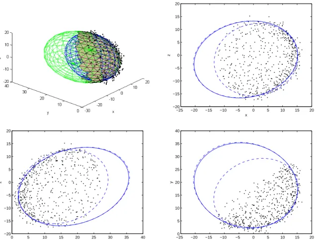
constraints. . . 34 2.6 Fitting an ellipsoid to noisy data. . . 43 3.1 Cluster assignments on some artificial data sets. . . 50 3.2 Data points and their associated foot points obtained by projecting the data points

onto the ellipse, minimizing geometric distance. . . 53 3.3 Comparison of manifold clustering algorithms. . . 56 3.4 Robustness of the proposed non-iterative manifold clustering algorithm in

re-sponse to increasing level of noise. . . 57 3.5 Asymmetric distance with spectral clustering. . . 62 4.1 The first 100 samples of the investigated Mackey–Glass chaotic process. . . 86 4.2 Discovering the input/output noise ratio using the Itakura–Saito matrix divergence. 89 5.1 Points extracted from the laser-scanned model of the Stanford Bunny. . . 92 5.2 Scattered points of the Stanford Bunny captured with at most quadratic 3D shapes. 93 A.1 Projection functionQ(t) for an ellipse. . . 115 A.2 Projection functionQ(t) for a hyperbola. . . 116 A.3 Projection functionQ(t) for a parabola. . . 118

(18)

(19)

C

HAPTER

1 Introduction

A recurring problem in engineering is constructing a computer model from a possibly large set of data. In fields such as computer vision, pattern recognition, image reconstruction, speech and audio processing, signal processing, modal and spectral analysis, data mining, system identification, econometrics or time series analysis, the goal is often to identify or describe the internal laws that govern a system rather than to predict its future behavior. In other words, one is interested in reconstructing how the measured variables are related given a set of observations. The amount and dimensionality of the observed data may be large yet one is often able to express the equation that relates data points in a succinct man-ner. In a system identification context, for instance, one could be interested in the parame-ters of a discrete-time dynamic system model, based on a measured input and output data sequence, contaminated with noise. In a pattern recognition context, on the other hand, one would seek to capture a set of unorganized data points with a number of simple shapes, such as lines, ellipses, parabolas, etc. While these tasks appear to be wildly different, they share some common properties, which outline the characteristics ofparametric errors-in-variablessystems:

• The relationships that characterize the system under investigation admit a structure. Even if the data accumulated may be large, the number of parameters is limited: the system can be explained by a set of relatively simple relationships, each known up to the parameters. A discrete-time dynamic system may be described by a low-order polynomial that relates the output variable with past values of the input and output variables, even if the data sequences may comprise of thousands of observations. Points obtained from a manufactured object by a laser scanner could be modeled with a cou-ple of quadric surfaces.

• There are no distinguished variables in general. The equation that relates data points has the implicit form fi mp(x)=0 rather than an explicit form y = fexp(z), i.e.

errors-in-variables systems have an inherent symmetry regarding the variables. For example, in the parametric description of an ellipseQ(x)=ax₁2+bx2₂−1=0 in canonical form, neither the componentx2, nory2has special significance. Implicit functions can

(20)

typ--6 -4 -2 0 2 4 -6 -4 -2 0 2 4 x x x x x x x x x x x -6 -4 -2 0 2 4 -6 -4 -2 0 2 4 x x x x x x x x x x x

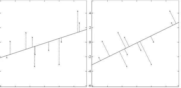
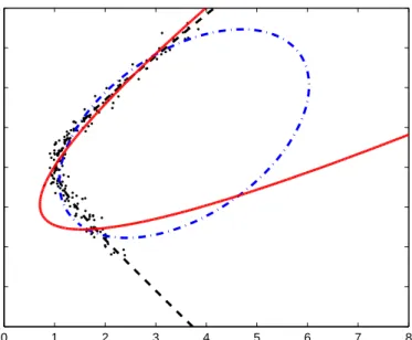
Figure 1.1: Visual comparison between the standard least-squares and the errors-in-variables ap-proach.

ically capture a wider range of systems, and can often result in a more succinct repre-sentation than an equivalent explicit formy=fexp(z) wherex>=

£

y z> ¤

. However, techniques applicable to the explicit representation do not necessarily carry over to the implicit one.

• The underlying data space is usually homogeneous and isotropic with no inherent co-ordinate system. The estimation process should be invariant to changes of the coor-dinate system with respect to which the data are described. For instance, in a three-dimensional scan, there is no special significance of any of the coordinatesx, y orz, data may be rotated and translated.

• Measured data is contaminated with noise. Unlike the usual assumption in statistics, there is in most cases no meaningful distinction between independent (noise-free) and dependent (noisy) variables. In the errors-in-variables context all variables are as-sumed to be measured quantities, hence contaminated with noise. Both the input and the output of the dynamic system is treated as a sequence of noisy measurements, and the points that are captured with a scanner are polluted with noise in all coordinates. Identifying the underlying relationship that governs a system gives us a compact represen-tation that is easier to manipulate and a key to understanding. For instance, a pattern recog-nition algorithm that exploits that an approximated 85% of manufactured objects can be modeled with quadratic surfaces [16], and subsequently reduces to fitting these surfaces, uses far fewer parameters than a primarily non-parametric approach that uses only locality information. Furthermore, the reverse-engineered model lends itself better to future trans-formations such as constructive solid geometry operations.

Figure 1.1 illustrates the difference between the standard least-squares approach in statis-tics and the errors-in-variables approach for linear data-fitting in two dimensions [20]. The

(21)

set of data at our disposal is identical in the two cases. The least-squares approach distin-guishes an independent variable (x-axis) and a dependent variable (y-axis). Any measure-ment error is assumed to concentrate in the dependent variable, hence the optimal solution is to fit a line that minimizes the error w.r.t. the dependent variable. In contrast, the errors-in-variables approach is symmetric: there is no distinction between independent and de-pendent variables. As observations are treated as polluted with noise w.r.t. any variable, the best-fit line can be vastly different from that in the standard least squares case. Apparently, the errors-in-variables approach is more suited to a situation in which we try to understand how a system works using a set of measurements, none of which can be treated as completely accurate. Obviously, the least-squares approach is a special case of the errors-in-variables approach where some variables take no error.

Depending on the structure imposed on the approximated model, multiple different es-timation problems can be outlined. Systems can be classified intostaticordynamicsystems whether observations are independent or coupled in time. The problem can be a pure pa-rameter estimationproblem where the solution is known up to a fixed number of free system parameters or anon-parametric problem where discovering a suitable model structure is part of the problem. In addition, parameter estimation problems can be further classified intolinearornonlinear, both in terms of data and parameters.

When the relationship is linear, standard tools in mathematics and statistics, such as sin-gular value decomposition, can be applied to static systems, and iterative algorithms may be formulated for dynamic systems. Nonlinearity in the system, however, makes it difficult to draw conclusions for the original (noise-free) relationship based on (noisy) measured vari-ables; traditional approaches may lead to substantial bias as additive noise contaminates nonlinear variables of the system. The objective of the thesis is to extend the results for lin-ear errors-in-variables systems to a relatively rich set of the nonlinlin-ear case when the system is captured by polynomial functions. This leads us to the following open questions:

• How can we extend the principles of methods developed with the usual statistical as-sumption to the errors-in-variables context? Moving from the asas-sumption of problem separation into independent (known accurately) and dependent (measured with error) variables to the (inseparable) errors-in-variables domain, a large number of additional unknown quantities are introduced into the model, often repositioning the problem in a more difficult context (e.g. multiple equivalent solutions and necessary normaliza-tion).

• How can we generalize existing methods for linear systems in the errors-in-variables framework to nonlinear systems? Linear systems usually reduce to a non-iterative so-lution but nonlinear systems typically demand an iterative approach where conver-gence and the choice of initial values are important issues.

• How can the errors-in-variables principles help us improve estimation accuracy while imposing only a moderate computational cost?

• How can existing errors-in-variables methods be improved to apply to a wider range of systems? Many existing methods have a limited applicability to general conditions, or demand excessively large samples or obtain reliable results.

(22)

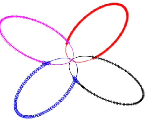
Figure 1.2:Identifying the decomposition of a complex curve.

• How can we incorporate estimation methods for nonlinear parametric errors-in-varia-bles systems in machine learning applications such as model construction from point clouds? Unlike parameter estimation problems where the structure of the problem is a priori known, reconstruction problems must discover a feasible partitioning of the data set into groups that exhibits a specific parametric relationship as well as estimate the unknown parameters for data within a group.

The thesis investigates algorithms related to identification and recognition problems that belong to the domain of nonlinear parametric errors-in-variables systems. We shall look into both static and dynamic (time-dependent) systems, with focus on low-order polynomial functions, and assume the noise that contaminates measurements is Gaussian. Contribu-tions address both the pure parametric case, where the system is known up to the unknown parameters, as well as the machine learning case, where we assume the system is known to comprise of a set of constituents, each captured with a well-known structure defined by a set of unknown parameters.

First, we venture onto the field of static systems where the estimation may be subject to constraints. In a computer vision application, for instance, one may be interested in fitting an ellipse rather than a general quadratic curve to an unorganized point set. Previous work in the computer vision domain showed how to integrate constraints such as the quadratic curve representing an ellipse (rather than e.g. a hyperbola) into the estimation but failed to adequately take into account the nonlinear distortions induced by noise. The method proposed in the thesis takes a step further, and incorporates constraints into parameter es-timation while canceling the effect of noise.

Second, we investigate a machine learning or reverse engineering application, namely clustering, where the system is originally built up of several constituents, each described by a polynomial relationship, more restrictively quadratic curves and surfaces, but only an un-organized set of noisy data is at our disposal, and we aim to discover the original structure of the system and estimate parameters of the constituents. Unlike standard parameter es-timation methods where the model to reconstruct is structured, i.e. is known up to a few free parameters to estimate, the problem is more challenging when structure discovery is part of the problem, i.e. a natural decomposition of the entity under study exists but is not

(23)

¯ uk _/_/ G(q)=B_A(₍q_q−−11)₎ ¯ yk_/_/ ˜ uk // Σ uk // y˜k _/_/ Σ yk _/_/

Figure 1.3:A linear dynamic discrete-time errors-in-variables system.

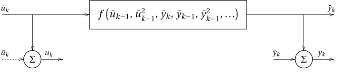
¯ uk _/_/ f ¡u¯k−1, ¯u2_k₋₁, ¯yk, ¯yk−1, ¯y_k2₋₁, . . . ¢ y¯k_/_/ ˜ uk // Σ uk // y˜k _/_/ Σ yk //

Figure 1.4:An example of a polynomial dynamic discrete-time errors-in-variables system.

known to us. Several algorithms exist that can tackle the so-called (multi-)subspace cluster-ing or hybrid linear modelcluster-ing problem, where the objective is to build a model where each partition of the data is captured by a linear relationship and the entire model is a compo-sition of these partitions. Not every data set, however, admits a decompocompo-sition into linear relationships, and applying linear methods to essentially nonlinear relationships loses the simplicity and explanation power of these methods. A natural generalization of subspace clustering is (multi-)manifold clustering, which we explore in this thesis, where each curved manifold is captured by some nonlinear (or more specifically, polynomial) relationship. Fig-ure 1.2 shows such a setup: a combination of points along four ellipses make up a complex curve. Here, the complex curve comprises of four independent quadratic curves, which the complex curve can be seen as a union of.

Finally, we explore dynamic systems, where we consider discrete-time but nonlinear sys-tems that can be re-cast in a linear setting using a lifting function. Figure 1.3 shows how a linear errors-in-variables system compares to a classical dynamic system setup in system identification. In the classical case, only system output is measured with noise, system in-put can be observed noise-free (i.e. no noise contribution by the dashed line), which is a well-understood problem. The case is more subtle when both the system input and output is contaminated with noise but many algorithms exist for the case when the ratio of input and output noise is at our disposal. The thesis takes a step further and deals with dynamic systems where the input and output are no longer related in a linear manner but captured by a polynomial function. Such a system model is shown in Figure 1.4. The thesis combines a generalization of the Koopmans–Levin method [65] with a nonlinear extension to the orig-inal Koopmans method [66]. The generalized Koopmans–Levin method is an approach to estimate parameters of a linear dynamic system with a scalable balance between accuracy

(24)

and computational cost, whereas the nonlinear extension to the Koopmans method gives a non-iterative approach to estimate parameters of a static system described by a polynomial function. The algorithm proposed in the thesis alloys the two approaches, and estimates pa-rameters of dynamic systems whose variables are related with a polynomial function from a set of data polluted with Gaussian noise.

A working implementation with several examples is essential to the popularization of any new methods. The results in this thesis are augmented with source code, which demonstrate the feasibility of the proposed algorithms.

(25)

C

HAPTER

2 Parameter estimation over point

clouds

Fitting a model to measured data that captures the underlying relationship, in particular, fit-ting (a certain a class of ) quadratic curves and surfaces (e.g. ellipses and ellipsoids) occurs frequently in computer vision, computer-aided design, pattern recognition and image pro-cessing applications. Unlike the large mass of scattered data acquired with some measuring device (e.g. a laser scanner), the curves and surfaces fitted to data can be represented with only a few parameters, which lends itself to compact storage and easier manipulation. In particular, low-order implicit curves and surfaces are a practical choice in grasping the rela-tionship since they are closed under several geometric operations (e.g. intersection, union, offset) while they offer a higher degree of smoothness than their counterparts with the same number of variables but cast in an explicit form, and may be preferred especially if the ob-ject under study itself is a composition of geometric shapes. It has been reported that 85% of manufactured objects can be modeled with quadratic surfaces [16], which highlights the significance of methods that can fit such surfaces to measured data.

The general estimation problem we face can be formalized using the notation f(¯xi)=0

where ¯xiis a vector of noise-free data,xi =x¯i+x˜iis a data vectori=1, . . . ,NwithNbeing the

number of data points, ˜xi is a noise contribution, and we seek to capture the relationshipf,

often referred to as a level-set function (or in this particular case, a zero-level set). However, if structural information is available as to the relationship f of the point set, the estimates can be improved by incorporating that information in the estimation procedure. Parametric estimation methods take this approach and come down to choosing an appropriate model and finding values for the model parameters. A general nonlinear parametric system takes the form

f(¯xi,g)=0

where ¯xi is a vector of noise-free data,gis a vector of model parameters (e.g. curve or

sur-face parameters), and f is a nonlinear function that relates data and parameters. From the formulation, it follows that the system is assumed structured, i.e. it is known up to (a few) model parameters. Our goal is to estimategfrom noisy samplesxi.

(26)

The field of parametric estimation methods targeting nonlinear systems is rather broad. Some approaches that do not aim at discovering the internal structure in the data employ techniques that allow sufficient flexibility of an approximating function ˆf to adapt to lo-cal features (using many components ing). A prominent example is spline-like approaches whereby a continuous curve with given order and possibly knot sequence is fit to the data points (gradually pulling the function ˆf towards data points), minimizing an error measure and the associated complexity of the curve. Even while these approaches are suitable for approximating the data but are of little help explaining the data: the spline itself does not facilitate understanding the underlying structure. Thus, we shall explore parameter estima-tion methods where low-order polynomial funcestima-tions such as quadratic curves (for 2D) and surfaces (for 3D) capture the relationship between data points.

Thus, it is natural to restrict our investigation to a narrower scope; we will discuss non-linear systems that assume a polynomial form in terms of data, which are captured by the implicit equation

fd at a(¯xi)>fpar(g)=0

where xi =x¯i+x˜i is a data vector i =1, . . . , N with N being the number of data points,

˜

xi ∼ N(0, C_σ2

x) is a noise contribution, g is a parameter vector. The (polynomial)

func-tion fd at a : Rn → Rm is the lifting function for data, mapping a data vector ¯xi ∈Rn into m-dimensional space, and the (polynomial) functionfp ar : Rp→Rm is the lifting function

for model parameters, mapping a parameter vectorg∈Rp intom-dimensional space. The matrixC_σ2 x=diag ¡ σ2 x ¢

is the noise covariance matrix for the homoskedastic normal (Gaus-sian) noiseN (i.e. noise has the same variance for all data points) whereσ2_x is a vector of variances for each component of an ˜xi.σ2xis assumed to be known up to scale, i.e.σ2x=µσ¯2x

where the vector ¯σ2_xis known but the scalarµis unknown. The noise covariance matrixC_σ2

x

is (in general) of full rank: there is no distinguished variable that we can observe noise-free, which is what we call the errors-in-variables approach.

Example 1. Observations of a static system transformed by a lifting function. Suppose we have a set of noisy data in two dimensions

xi=

£

xi yi 1

¤> and our goal is to fit an ellipse minimizing algebraic distance

e= 1 N N X i=1 ¡ f(xi,g)¢2.

The parameters of the ellipse are

g=£ a b c p q d ¤> where we ideally have

ax2+bx y+c y2+px+q y+d=0 s.t.b2<ac

where the constraint ensures the estimator always produces an ellipse. Our lifting function for data is then

fd at a(xi)=

£

x2_i xiyi y_i2 xi yi 1

(27)

and the lifting function of parameters is the identity mapping fpar(g)=g.

♣ The rest of the chapter is structured as follows. Section 2.1 introduces the unconstrained fitting problem in which the objective is either to minimize a geometric or an algebraic dis-tance, but without any ancillary constraints. Sections 2.1.1 and 2.1.2 cover maximum like-lihood methods, which minimize Euclidean distance of the scattered points to the curve or surface being estimated, whereas Sections 2.1.3, 2.1.4 and 2.1.5 survey related work that are based on simpler and computationally less expensive approaches, which reduce to solving a regular or a generalized eigenvalue problem. Section 2.1.6 discusses the nonlinear Koop-mans method, whose principles are integral to the noise cancellation step part of the con-strained fitting algorithm proposed in this thesis, with numerical improvements that fur-ther reduce computational cost. Section 2.2 concentrates on fitting quadratic curves and surfaces subject to constraints, with a two-stage algorithm comprising of a noise cancella-tion step and a constrained fitting step, which is one of the main results in this thesis. Sec-tion 2.2.1 uses a known numerical technique to reduce matrix dimensions to the size of the nonzero part of the constraint matrix, whereas Sections 2.2.2, 2.2.3 and 2.2.4 describe al-gorithms for fitting various classes of quadratic curves and surfaces. While the alal-gorithms themselves are known results, the context in which they are used, namely, operating on a noise-compensated matrix, is a new contribution of this thesis, and formulated as a single algorithm in Section 2.2.5. The new algorithm in Section 2.2.5 is also a key ingredient to another major result in this thesis covered in Chapter 3, a clustering method fitting at most quadratic curves and surfaces, where an inexpensive yet effective estimation method is in-dispensable.

2.1 Unconstrained fitting

An important class of fitting problems falls into the category of unconstrained fitting where no constraints are imposed other than the implicit equation

fp ar

¡ g¢

fd at a(¯xi)=θ>z¯i=0.

Here, we seek to find the bestgthat minimizes the fitting error using noisy samplesxi=x¯i+x˜i

where ¯xi is noise-free data and ˜xi is a noise contribution, and ¯zi =fd at a(¯xi). For simplicity,

we assume thatfp ar

¡ g¢

is an identity transformation and thusθ=g.

One possible way to estimategfromxi is to use geometric distance, and employ

maxi-mum likelihood methods, and minimize e= 1 N N X i=1 d_i2

wheredi measures the distance from the noisy point xi to the curve or surface f(x,g)=

(28)

C_σ2

x =σ

2_I_{(i.e. all vector components are contaminated with equal amount of noise) or in} general Mahalanobis distance (a scale-invariant distance measure that takes into account correlations inC_σ2

x).

Approaches that aim at minimizing Euclidean or Mahalanobis distance aregeometric fit-ting methods, and include maximum likelihood, approximate likelihood [49, 18] or renor-malization methods [36]. While highly accurate, they lead to an iterative formulation that may converge slowly (or even diverge) in some situations, and always requires a feasible ini-tialization. More substantial levels of noise may impact convergence and have an adverse effect on estimation accuracy.

A more robust approach than geometric fitting is to use algebraic distance e= 1 N N X i=1 ¡ f(xi,g)¢2

where noisy points are substituted into the curve or surface equation. Thealgebraic fit mini-mizes this substitution error, which yields a fast, non-iterative approach that is typically less accurate than geometric fit. With proper compensation for the error induced by noise, how-ever, it is possible to reduce adverse effects, and construct estimation methods, such as the nonlinear Koopmans method [66] or consistent algebraic least squares [42, 48], that achieve accuracy similar to maximum likelihood estimation, at much lower computational cost.

For the purposes of parameter estimation, we assume that the data has zero mean and has been normalized to its root mean square (RMS), which is meant to reduce numerical errors [17]. For each dimensionxof the data set, this means

mx = 1 N N X i=1 xi xi ← xi−mx s σx ← σx s and likewise for all other dimensionsy,z, etc. where

s= s 1 2n n X i=1 n (xi−mx)2+ ¡ yi−my¢2 o

for two dimensions and s= s 1 3n n X i=1 n (xi−mx)2+ ¡ yi−my¢2+(zi−mz)2 o

for three dimensions. Reducing data spread also reduces the additive noise on components ofxi and the noise covariance matrix has to be updated accordingly. Translation and

scal-ing also dilates model parametersg. For instance, when estimating quadratic curves in two dimensions with the lifting function

fd at a(xi)=

£

x2_i xiyi y_i2 xi yi 1

(29)

parameters

g>=£ g1 g2 g3 g4 g5 g6 ¤

in the original space are recovered as follows: g1 ← g1s2 g2 ← g2s2 g3 ← g3s2 g4 ← −2g1s2mx−g2s2my+g4s3 g5 ← −g2s2mx−2g3s2my+g5s3 g6 ← g1s2m2x+g2s2mxmy+g3s2m2y−g4s3mx−g5s3my+g6s4.

2.1.1 Maximum likelihood estimation

Estimating parameters of a linear system where all data points are related by the same func-tion but polluted by Gaussian noise with a known structure is the well-understood and widely-used method of total least-squares fitting [35], solved as either an eigenvalue problem or a computationally more robust singular value problem, which yields maximum likelihood es-timates. Without a priori information (in addition to preliminary structural information), maximum likelihood methods deliver the best possible estimates for the model parameters based on measured data of the system under investigation. In the maximum likelihood con-text, we seek to maximize the (joint) probability (compound probability density function)

p(x|g, ¯x)=

N

Y

i=1

p(xi|g, ¯xi)

over the parameter vectorgwherexis a vector of all (observed) data pointsxi, ¯xis a vector

of all (unknown) noise-free data points ¯xi, and p(xi|g, ¯xi)= 1 r (2π)dim ³ C_σ2 x ´ det ³ C_σ2 x ´ exp µ −1 2(xi−x¯i) >_C−1 σ2 x(xi−x¯i) ¶ (2.1)

in which the noise covariance matrixC_σ2

x (available up to scale) is at our disposal, and we

have assumed that the noise contributions over data pointxi are independent and

identi-cally distributed. (dimC_σ2

x equals the number of components inxi and ¯xi.) While tackled

relatively easily for the linear case, the nonlinear case poses difficulty with the exploding number of unknowns.

Removing the leading constant term in (2.1) we get p(xi|g, ¯xi)∝exp ½ −1 2(xi−x¯i) >_C−1 σ2 x(xi−x¯i) ¾

leading to the log likelihood cost function that takes the form

J= N X i=1 (xi−x¯i)>C−_σ12 x(xi−x¯i) s.t.g >_f d at a(¯xi)=0 (2.2)

(30)

for eachi =1, . . . ,N wherefd at a(¯xi) is a lifting of ¯xi. Minimizing the constrained function

(2.2) (where the constraint enforces the model) is equivalent according to the method of Lagrange multipliers to minimizing the unconstrained function

J = N X i=1 (xi−x¯i)>C−_σ12 x(xi−x¯i) (2.3) + N X i=1 ηig>fd at a(¯xi)

When the lifting functionfd at a is linear, the constraints can be substituted directly into

the constrained equation (2.2) and produce a simpler form. However, this is unfortunately not possible in the nonlinear case and minimizing (2.3) w.r.t. all variables is burdensome. Iterative methods, however, may offer a means to tackle the problem.

On the other hand, the objective function

J= N X i=1 (xi−x¯i)>C−_σ12 x(xi−x¯i) can be interpreted as J= N X i=1 d2 ³ xi−x¯i,C_σ2 x ´ = N X i=1 d_C2(xi−x¯i) (2.4) where d(a−b,C)= q (a−b)>C−1_(a₋_b)

is the so-called Mahalanobis distance between data vectorsaandb(or Euclidean distance if C=I). In the particular case, this means that the distance between observed data pointsxi

and the (unknown) true data points ¯xiis to be minimized, given the constraintg>fd at a(¯xi)=

0.

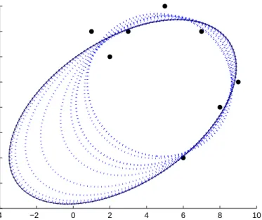
This formulation allows us to set up an iterative procedure whereby the curve or sur-face to be found is pulled towards the observed data points, minimizing the distance metric (Figure 2.1). In fact, we seek the minimum of (2.4), which is a nonlinear least-squares opti-mization problem, since the distance depends on the parametersgin a nonlinear manner. If we compute

∂

∂gdC(xi−x¯i)

we may use gradient-based minimization (e.g. Levenberg–Marquardt algorithm) to find the local minimum. If seeded with an estimate for gthat is close enough to the solution, the value ofgis readily found.

Unfortunately, values of ¯xi are not at our disposal but given a curve or surface defined

with the (current) parameters g, observed data pointsxi can be projected to the curve or

surface to obtain so-called foot points, i.e. points that satisfy the constraintg>fd at a(¯xi)=0,

in each step. The most natural choice for the projection is to minimize geometric distance, i.e. ¯ xi=arg min x dC ¡ xi−x(g) ¢ .

(31)

−4 −2 0 2 4 6 8 10 0 1 2 3 4 5 6 7 8

Figure 2.1:Iterative maximum likelihood estimation. The initial curve that gives a rough parameter estimate is gradually attracted towards the final solution (continuous line).

The expressionx(g) indicates thatxmust satisfyg>fd at a(x)=0 wheregandfd at a are given.

This way, we can compute the objective function valueJ and its gradient _∂∂_gJ in each step. The entire algorithm can be summarized as follows:

g=arg min g J(g)=arg ming N X i=1 dC ³ xi−arg min x dC ¡ xi−x(g) ¢´ .

There are two important implications of this approach:

1. Good-enough initial estimates forgthat are close to the solution are crucial such that the local minimum obtained in the process is also a global minimum.

2. Fast projection algorithms are needed such that ¯ xi=arg min x dC ¡ xi−x(g) ¢

can be obtained in an economical way.

The problem of initialization is tackled with relatively highly accurate but non-iterative meth-ods such as Taubin’s method (see [61] and Section 2.1.4) or consistent algebraic least squares (see [66, 42, 48] and Section 2.1.6). Projection, in general, requires solving polynomial equa-tions but fast algorithms exist for the special case of projecting to at most quadratic curves and surfaces (covered in more depth in Section 3.3). This highlights that despite the accuracy of the maximum likelihood method, non-iterative low-cost methods with similar accuracy are much desired.

(32)

2.1.2 Approximated maximum likelihood estimation

The approximated maximum likelihood (AML) estimation method [18] is one of the various computational schemes that have been proposed for estimating curve or surface parame-ters, with accuracy close to those obtained by maximum likelihood methods. As its name suggests, the method does not minimize the unconstrained maximum log-likelihood func-tion (2.3) but a simplificafunc-tion of it. First, the likelihood funcfunc-tion is formulated in an alter-native way, then functions of unobservable noise-free variables ¯xi are substituted with their

approximations obtained from available noisy dataxi. Finally, an iterative scheme is

em-ployed to yield parameter estimates in a few iterations. Even while the approximated and the true maximum log-likelihood function are seldom minimized at the same objective function variable value, the estimates are close in practice.

The key to simplifying the objective function (2.3) of maximum likelihood estimation is its alternative form, to be developed based on [18].

The method of Lagrange multipliers implies that the gradient (column vector of partial derivatives) of (xi−w)>C−_σ21

x(xi−w) w.r.t.wis proportional to the gradient ofg

>_f

d at a(w)

pro-vided that both these gradients are evaluated at ¯xi. Comparing the gradients, it follows that

C−_σ21

x(xi−x¯i)=λig

>_∂

xfd at a(¯xi) (2.5)

for some scalarλi. Multiplying both sides of the equation byC_σ2

x andg >_∂ xfd at a(¯xi), we find g>∂xfd at a(¯xi) (xi−x¯i)=λig> ³ ∂xfd at a(¯xi)C_σ2 x∂xf > d at a(¯xi) ´ g and hence λi= g>∂xfd at a(¯xi) (xi−x¯i) g>_∂ xfd at a(¯xi)C_σ2 x∂xf > d at a(¯xi)g (2.6) On the other hand, multiplying both sides of (2.5) by (xi−x¯i)>, we obtain

(xi−x¯i)>C−_σ12

x(xi−x¯i)=λi(xi−x¯i)

>_∂

xf>d at a(¯xi)g

Substituting the value ofλi from (2.6) into this equation, we may conclude that

(xi−x¯i)>C−_σ12 x(xi−x¯i)= g>∂xfd at a(¯xi) (xi−x¯i) (xi−x¯i)>∂xf>_{d at a}(¯xi)g g>_∂_x_f d at a(¯xi)C_σ2 x∂xf > d at a(¯xi)g (2.7)

Consider the Taylor expansion of theγth component offd at a(x) about any particularw(the

observation indexi is omitted fromxfor clarity, the subscript is the component index inxor w): f_γ(x1,· · ·,xd)= ∞ X n1=0 · · · ∞ X nd=0 ∂n1 ∂xn1 1 · · · ∂ nd ∂xnd d f_γ(w1,· · ·,wd) n1!· · ·nd! (x1−w1)n1 · · ·(xd−wd)nd

which for a second order approximation simplifies to f_γ(x)≈f_γ(w)+∂xfγ(w)(x−w)+1

2(x−w)

>_∂

(33)

or rearranged ∂xfγ(w)(x−w)=fγ(x)−fγ(w)− 1 2(x−w) >_∂ xxfγ(w)(x−w)

Settingw=x¯i and taking into account thatg>fd at a(¯xi)=0 yields

g>∂xfd at a(¯xi) (xi−x¯i)=g>(fd at a(xi)−r(xi, ¯xi))

wherer is a term encapsulating all second and higher order derivatives. With this, (2.7) can be rewritten as (xi−x¯i)>C−_σ21 x(xi−x¯i)= © g>(fd at a(xi)−r(xi, ¯xi))ª2 g>_∂_x_f_{d at a}_(¯_x_i₎_C σ2 x∂xf > d at a(¯xi)g

leading to the rearranged maximum likelihood objective function

The reformulated maximum likelihood objective function (2.8) easily lends itself to ap-proximations. A primary obstacle to direct minimization of (2.8) is that neither∂xfd at a(¯xi)

norr(xi, ¯xi) can be expressed as they depend on unknown noise-free observations ¯xi. In

contrast, they have to be substituted with∂xfd at a(xi) andr(xi) that are computed from noisy

observations. Formally, this is reflected in the approximated cost function [18]

J= N X i=1 g>(fd at a(xi)−rˆ(xi)) (fd at a(xi)−rˆ(xi))>g g>_∂_xˆ_f_{d at a}_(x_i₎_C σ2 x∂x ˆ_f> d at a(xi)Cσ2xg (2.9)

where ˆfd at a(xi) indicates approximation offd at a(xi) and ˆr(xi) indicates approximation of r(xi).

As compared to the original maximum likelihood function, (2.9) takes the following sim-plifications:

• The gradient∂xfd at a(¯xi) is approximated with the gradient∂xfd at a(xi) computed based

on noisy observations.

• Similarly to gradients, the residual components r(xi, ¯xi) that result from the Taylor

series expansion depend on the unknown true observations ¯xi. If the lifting function

(34)

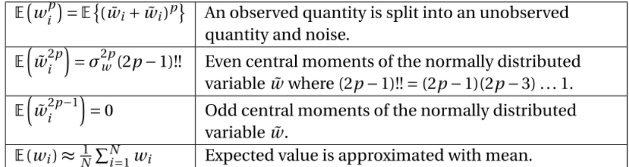
cancel if we apply expected value: r(xi, ¯xi) = 1 2(x−y) >_∂ xxfd at a(y)(x−y) = trace µ 1 2(x−y) >_∂ xxfd at a(y)(x−y) ¶ Er(xi,x0,i) = E ½ trace µ 1 2(x−y) >_∂ xxfd at a(y)(x−y) ¶¾ = 1 2E © trace¡ (x−y)(x−y)>∂xxfd at a(y) ¢ª = 1 2trace ¡ E© (x−y)(x−y)>ª∂xxfd at a(y) ¢ = 1 2trace ¡ C∂xxfd at a(y) ¢

This simplification applies to higher order terms as well, but dependence on the obser-vations will not vanish. As dependence on unknown true obserobser-vations is not desired, they have to be expressed in terms of actual observations, in the same fashion as for gradients.

One way to minimize (2.9) is to employ direct search methods. A more robust technique is to use an iterative scheme. For this end, introduce the compact notation

J= N X i=1 g>Aig g>_B ig

so that for the approximated likelihood function to attain a minimum we need

∂gJ= N X i=1 1 g>_B_i_gAig− N X i=1 g>Aig ¡ g>_B ig¢2 Big=0.

Let us introduce the substitutions

Mg = N X i=1 1 g>_B_i_gAi Ng = N X i=1 g>Aig ¡ g>_B ig¢2 Bi Xg = Mg−Ng so that we have ∂gJ=Mgg−Ngg=Xgg=0. (2.10)

Finally, the solution to (2.10) can be iteratively sought in several ways. One possibility is the so-called fundamental numerical scheme [18], which seeks the solution as the eigenvector corresponding to the smallest eigenvalue in the eigenvalue problem

(35)

This approach is inspired by the fact that a vectorgsatisfies (2.10) if and only if it is a solution to the ordinary eigenvalue problem (2.11) corresponding to the eigenvalueµ=0. Letg(k)be the current approximate solution in iterationk, andXg(k) be computed with the substitution ofg(k). In a single iteration, the updated solutiong(k+1)is chosen from that eigenspace ofXg(k) that most closely approximates the null space ofXg, which corresponds to the eigenvalue

closest to zero in absolute value. In other words, we solve a series of eigenvalue problems Xg(k)g(k+1)=µ(k+1)g(k+1). (2.12) Another possibility is to seek the eigenvalue closest to 1 in the eigenvalue problem as in [49]

Mgξ=µNgξ

leading to a similar series of eigenvalue problems

Mg(k)g(k+1)=µ(k+1)Ng(k)g(k+1). (2.13) Like all iterative schemes, (2.11) and (2.13) require feasible initialization to avoid slow convergence or divergence. Less accurate but non-iterative methods help provide initial es-timates that may already be close to the final solution.

2.1.3 Nonlinear least-squares methods

As previously seen, maximum likelihood methods are solved with a gradient search or an iterative scheme, where the former needs proper initialization and the latter may diverge, especially in the presence of large noise. The principle of nonlinear least-squares methods is to minimize the residual sum of squares (RSS), or in other words, the sum of the squares of errors that result when we substitute data into the estimated objective function:

ˆ g=arg min g N X i=1 ¡ f(xi,g)¢2.

The motivation behind the approach is that standard least-squares optimization methods can be employed to find a minimum, and when true values of data and parameters are sub-stituted into the expression, we get zero error:

N

X

i=1 ¡

f(¯xi,g)¢2=0.

Let a linearization (lifting) of 2D data be

z>_i =£ x_i2 xiyi y_i2 xi yi 1

¤

(2.14) which captures quadratic curves, and a linearization (lifting) of 3D data be

z>_i =£ x_i2 y_i2 z_i2 yizi xizi xiyi xi yi zi 1

¤

(36)

which captures quadratic surfaces wherexi, yi andzi are data point coordinates in two or

three dimensions. (The same principles apply for higher-order polynomials.) The sample covariance matrix is then

D= 1 N X i Ã zi− 1 N X j zj ! Ã zi− 1 N X j zj !> . The least-squares solution then solves the eigenvalue problem

Dg=λg for the minimum eigenvalueλ.

Unfortunately, simple as it is, directly minimizing algebraic error is statistically inaccu-rate and leads to heavily biased estimates. As apparent from (2.14) and (2.15) the effect of noise on various components may nonlinear, such as forx2in (2.14) where

z>_i = h ( ¯xi+x˜i)2 ( ¯xi+x˜i) ¡ ¯ yi+y˜i ¢ ¡ ¯ yi+y˜i¢2 x¯i+x˜i y¯i+y˜i 1 i .

This must be taken into account in devising such estimation schemes. This motivates an approach to maintain the simplicity of least-squares methods yet combat their statistical inaccuracy, which can be accomplished with a noise cancellation scheme that removes the distortion effects of noise (as much as possible).

2.1.4 Estimation using geometric approximation

Estimates obtained with the least-squares approach are statistically inaccurate or biased [73]. A more robust way is to use a linear approximation of the geometric distance and min-imize J= N X i=1 ¡ f(xi,g)¢2 ° °∇f(x_i,g) ° ° 2 (2.16)

where the operator ∇ = h ∂ ∂x ∂∂y i for 2D and ∇ = h ∂ ∂x ∂∂y ∂∂z i for 3D. Unfortunately, (2.16) cannot be solved without iterations but a further simplification of it, called Taubin’s method [61] J= PN i=1 ¡ f(xi,g)¢2 PN i=1 ° °∇f(x_i,g) ° ° 2

lends itself to a non-iterative solution. In two dimensions, for instance,

N X i=1 ¡ f(xi,yi,g)¢2 = g> N X i=1 ³ £ x2 x y y2 x y 1 ¤>£ x2 x y y2 x y 1 ¤´ g N X i=1 ° °∇f(x_i, y_i,g) ° ° 2 = g> N X i=1 Ã · 2x y 0 1 0 0 0 x 2y 0 1 0 ¸>· 2x y 0 1 0 0 0 x 2y 0 1 0 ¸! g

such that the problem can be formulated as J=g

>_Ag

(37)

−4 −2 0 2 4 6 8 10 0 1 2 3 4 5 6 7 8

Figure 2.2: Comparison of maximum likelihood (continuous line), nonlinear least-squares (dotted line) and Taubin’s (dashed line) ellipse fitting methods to a set of two-dimensional coordinates.

with°°g °

°=1 and solved as a generalized eigenvector problem g>Ag=µg>Bg.

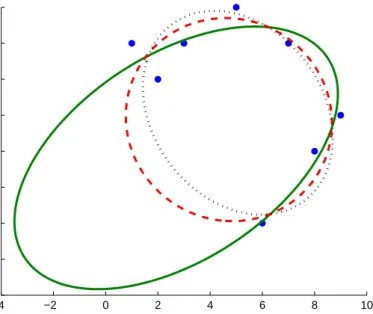
The solution ˆg, as previously seen, is the eigenvector that belongs to the smallest eigenvalue. Figure 2.2 compares various quadratic curve fitting methods to a set of two-dimensional data points with coordinates (1;7), (2;6), (5;8), (7;7), (9;5), (3;7), (6;2) and (8;4). The best-fit ellipse obtained with the maximum likelihood method (Section 2.1.1), which minimizes the sum of squares of (signed) distances to the quadratic curve foot points using the Levenberg– Marquardt method, is shown in continuous line, whereas the iterative methods non-linear least-squares fit (Section 2.1.3) and estimation with geometric approximation using Taubin’s fit (Section 2.1.4), are shown in dotted line and dashed line, respectively. The figure highlights that there might be substantial difference between the fit obtained with geometric distance and algebraic distance minimization.

2.1.5 Hyper-accurate methods

As we have seen, the ordinary least squares method solves the eigenvalue problem Dg=λg

for the minimum eigenvalueλ, effectively minimizing algebraic (substitution) error. How-ever, we may reformulate the above problem as

(38)

introducing a properly chosen normalization matrixQ. For ordinary least squares,Q=Ibut hyper-accurate methods chooseQsuch that higher-order bias terms induced by noise are canceled. This allows these (non-iterative) methods to completely eliminate estimation bias in ˆgand reduce variance [39], even if they do not attain the theoretical lower bound.1

Let

zi =

£

x_i2 2xiyi y_i2 2f0xi 2f0yi f₀2

¤

wheref0is a scaling constant in the order of (mean-free)xi andyi,

D= 1 N N X i=1 ziz>_i , and Vi=4          x x y 0 f0x 0 0 x y x2+y2 x y f0y f0x 0 0 x y y2 0 f0y 0 f0x f0y 0 f₀2 0 0 0 f0x f0y 0 f₀2 0 0 0 0 0 0 0         

which is what Taubin’s method effectively uses as normalization matrix. (For Taubin’s method, Q=_N1PN

i=1Vi.)

The normalization matrix for hyper-accurate fitting [39] is calculated as

Q= 1 N N X i=1 Vi+2S © zce>1,3 ª − 1 N2 N X i=1 ³ trace³D†Vi ´ ziz>_i + ³ z>_i D†zi ´ Vi+2S n ViD†ziz>_i o´ where zc = 1 N X i zi e>_1,3 = £ 1 0 1 0 0 0 ¤ and the symbolS denotes symmetrization

S {A}=1 2 ¡

A+A>¢ .

Hyper-accurate methods are preferred when the noise level is low. For higher noise level, consistent algebraic least squares (introduced in Section 2.1.6), is a more appropriate choice, which also uses fewer matrix operations and is nearly as accurate as hyper-accurate meth-ods.

1_{This theoretical lower bound is called the Kanatani–Cramer–Rao lower bound}_C K C R

¡

ˆ

g¢

and will be covered in more detail in Section 2.1.7. Permitting iterative algorithms with an adaptive choice of the normalization matrixQ, as in [5], it is possible to both entirely eliminate the bias in ˆgand achieve the theoretically lowest varianceCK C R¡gˆ¢.

(39)

2.1.6 Nonlinear Koopmans estimator

As previously seen, estimation strategies may be grouped into two coarse categories. High-accuracymethods, such as maximum likelihood or approximated maximum likelihood esti-mation, are close to the best possible estimate that can be obtained from the measured data but are computationally more expensive and require proper initialization. Low-accuracy methods, such as least squares or Taubin’s method, on the other hand, are easy to com-pute and require no initialization but are not nearly as accurate. A method that alloys the strengths of high-accuracy methods and mitigates the drawbacks of low-accuracy methods, even in the context of large noise level, is therefore much sought after. In particular, non-iterative schemes, even if they are not strictly optimal [39], can still deliver accurate esti-mates, and avoid any possibility of divergence inherent to iterative algorithms, especially in the presence of high levels of noise.

The principle of the nonlinear Koopmans estimator (also known as nonlinear extension to the Koopmans method [66] and consistent algebraic least squares [42, 48]), is to build the sample data covariance matrix from data subject to the lifting functionfd at a and use an

appropriate (pre-computed) noise covariance matrix to cancel the matrix rank-increase in-duced by measurement noise. Loosely speaking, the method tries to match the sample data covariance matrix with the theoretical noise covariance matrix that corresponds to measure-ment noise. Like withAMLin Section 2.1.2, the noise covariance matrix depends on ¯xi, which

are unknown, but can be approximated withxi, which are available.

When the lifting function is an identity mapping, the estimation problem is captured by the simple linear relationship

g>x=0.

The original work of Koopmans [40] addressed this estimation problem, and proposed a non-iterative but fairly inaccurate method to estimate model parameters from second-order statistical characteristics. The estimation method matches the data covariance matrix with the conceptual noise covariance matrix. The underlying assumption is that were it not for the noise present in observationsxi, the data covariance matrix would be a singular

ma-trix. Thus, finding the eigenvector of the data covariance matrix with respect to a noise co-variance matrix with the smallest-magnitude eigenvalue, parameter estimates can be found [66, 42, 48].

For convenience, let us introduce the (sample) data matrix and the (sample) data covari-ance matrix.

Definition 1. Data matrix.

X>=£ x1 x2 x3 . . . xN

¤

■ Definition 2. (Sample) data covariance matrix.