City, University of London Institutional Repository
Citation
:
Mammen, E., Nielsen, J. P. ORCID: 0000-0002-2798-0817, Scholz, M. and
Sperlich, S. (2019). Conditional variance forecasts for long-term stock returns. Risks, 7(4),
113.. doi: 10.3390/risks7040113
This is the published version of the paper.
This version of the publication may differ from the final published
version.
Permanent repository link:
http://openaccess.city.ac.uk/id/eprint/23329/
Link to published version
:
http://dx.doi.org/10.3390/risks7040113
Copyright and reuse:
City Research Online aims to make research
outputs of City, University of London available to a wider audience.
Copyright and Moral Rights remain with the author(s) and/or copyright
holders. URLs from City Research Online may be freely distributed and
linked to.
City Research Online: http://openaccess.city.ac.uk/ [email protected]
Article
Conditional Variance Forecasts for Long-Term
Stock Returns
Enno Mammen1, Jens Perch Nielsen2 , Michael Scholz3,* and Stefan Sperlich4
1 Institute for Applied Mathematics, Heidelberg University, Im Neuenheimer Feld 205, 69120 Heidelberg, Germany; [email protected]
2 Faculty of Actuarial Science and Insurance, Cass Business School, 106 Bunhill Row, London EC1Y 8TZ, UK; [email protected]
3 Department of Economics, University of Graz, Universitätsstraße 15/F4, 8010 Graz, Austria
4 Geneva School of Economics and Management, Université de Genève, Bd du Pont d’Arve 40, 1211 Genève, Switzerland; [email protected]
* Correspondence: [email protected]; Tel.: +43-316-380-7112
Received: 20 August 2019; Accepted: 29 October 2019; Published: 5 November 2019
Abstract:In this paper, we apply machine learning to forecast the conditional variance of long-term stock returns measured in excess of different benchmarks, considering the short- and long-term interest rate, the earnings-by-price ratio, and the inflation rate. In particular, we apply in a two-step procedure a fully nonparametric local-linear smoother and choose the set of covariates as well as the smoothing parameters via cross-validation. We find that volatility forecastability is much less important at longer horizons regardless of the chosen model and that the homoscedastic historical average of the squared return prediction errors gives an adequate approximation of the unobserved realised conditional variance for both the one-year and five-year horizon.
Keywords: benchmark; cross-validation; prediction; stock return volatility; long-term forecasts; overlapping returns; autocorrelation
JEL Classification:C14; C53; C58; G17; G22
1. Introduction
The volatility of financial assets has important implications for the theory and practice of asset pricing, portfolio selection, risk management, and market-timing strategies. Therefore, it is of fundamental interest to measure ex ante, or forecast successfully, the conditional variance of returns. Of course, the evaluation of the latter and the forecasting itself have been complicated by
the unobservability of the realised conditional variance (Galbraith and Kisinbay 2005). An extensive
amount of research is engaged in analysing the distributional and dynamic properties of stock market
volatility; see, for example,Andersen et al.(2001) and citations therein. The standard approaches
applied include parametric (G)ARCH-type or stochastic volatility models and estimate the underlying returns based on specific distributional assumptions. Alternatives, especially for data of higher
frequency, are based on constructing model-free estimates of ex-postrealizedvolatilities by adding up
the squares and cross-products of intraday high-frequency returns (Andersen et al. 2001).
The present paper instead uses annual U.S. stock market data to construct excess stock returns at the one-year and five-year horizon and to examine their model-based variance forecasts. Note that the risk depends on the investment horizon considered and that different horizons are
relevant for different applications (Christoffersen and Diebold 2000). Little is known about the
forecastability of variance at horizons beyond a year. Here, we take the long-term actuarial view
and extend the work ofKyriakou et al.(2019a,2019b). In a two-step procedure, we first apply machine learning (ML) to predict stock returns in excess of different benchmarks, considering the short- and long-term interest rate, the earnings-by-price ratio, and the inflation rate. Second, the squared residuals are used to analyse model-based volatility forecastability. Here, we compare these forecasts with the forecast implicit in the unconditional residual variance, as proposed, for example, byGalbraith and Kisinbay(2005). We find that volatility forecastability is much less important at longer horizons regardless of the chosen model and that the homoscedastic historical average of the squared return prediction errors gives an adequate approximation of the unobserved realised conditional variance for both the one-year and five-year horizon.
Our preferred ML technique applied in this paper is local-linear smoothing in combination with
a leave-k-out cross-validation for the following reasons.1 First, we are interested in longer-horizon
stock returns based on annual observations and their volatility. Thus, we are not in the high-frequency context where the number of observations is huge and the set of possible predictive variable combinations is enormous (and, thus, dimension reduction or shrinkage are indispensable). Our data set is, instead, sparse and a careful imposition of structure to the statistical modelling process is much
more promising, as shown, for example, byNielsen and Sperlich(2003) andScholz et al.(2015,2016).
Second, the evidence of stock return predictability is much stronger once one allows for nonlinear
functions as documented, for example, inLettau and Van Nieuwerburgh(2008),Chen and Hong(2010),
orCheng et al.(2019). Thus, the local-linear smoother is ideally suited as it can estimate a linear function—the classical benchmark in this context—without any bias. Finally, our procedures are analytically well studied, i.e., sound and rigorous, statistical tools which let us operate in a glasshouse,
not in a black box—in contrast to other fancier but less clear ML methods.2
Note further that longer horizons are important to long-term investors, such as pension funds or market participants saving for distant payoffs. These investors are generally willing to take on more risk for higher rewards and, thus, volatility forecastability is for them of fundamental
interest.Rapach and Zhou(2013) show that longer horizons tend to produce better estimates than
shorter horizons, whileMunk and Rangvid(2018) point out that major finance houses today use longer
horizons—up to ten years—to stabilise and improve future predictions. In our paper, we exemplarily
concentrate on the one-year and five-year view.3However, shorter horizons based on monthly, weekly,
or even daily data do not seem to provide the pension saver with good information about future income as a pensioner. Therefore, these type of short-term predictions—sometimes called investment robots—are not suitable when a pensioner should define his or her risk appetite.
The remaining of this paper is organized as follows. Section2presents our framework for the
purpose of conditional variance prediction. We define the underlying financial model, introduce our two-step procedure, and present our validation criterion for model selection. In addition, we review different ways of estimating the conditional variance and discuss bootstrap-tests for the null hypothesis
of no predictability. In Section3, we provide a description of our data set and of our empirical findings
from different validated scenarios: (i) a single benchmarking approach that uses the dependent variable transformed with the benchmark, and (ii) the case where both the independent and dependent variables are transformed with the benchmark (full benchmarking approach). Finally, we take the
1 Our methodology of validating a fully nonparametric structure can be viewed as one of the simplest and therefore also most
transparent version of machine learning; see Section 2 ofKyriakou et al.(2019a) for more details justifying the label machine
learning for our approach.
2 Note that the use of a different ML method would come with the cost of losing interpretability, smoothness, or flexibility
due to restrictions on the functional form. A comparison of different ML techniques in finding that one which gives the best predictions, wins an investment horse-race out-of-sample, or being the most robust method over different periods is out of the scope of our work.
3 The choice of the one-year horizon is related to the frequency of the data. In contrast, the five-year horizon is arbitrary but is
intended to be a starting point for actuarial long-term models for real-income savings. Other horizons and related questions remain for future research.
long-term view and comment on real income pension prediction. Section4summarizes the key points of our analysis and concludes the paper.
2. A Framework for Conditional Variance Prediction
In this section, we focus on nonlinear predictive relationships between squared residuals of
model-based predicted stock returns over the nextT years in excess of a benchmark and a set of
explanatory variables. Our aim is the investigation of different benchmark models and their volatility predictability over return horizons of one year and five years. We consider four different benchmarks: the short- and the long-term interest rate, the earnings-by-price ratio, and the inflation rate.
2.1. One-Year Predictions
LetPt denote the (nominal) stock price at the end of year tand Dt the (nominal) dividends
paid during yeart. We investigate stock returnsSt= (Pt+Dt)/Pt−1in excess (log-scale) of a given
benchmarkBt(−A1):
Yt(A)=ln St
B(t−A1), (1)
whereA∈ {R,L,E,C}with, respectively,
B(tR)=1+ Rt 100, B (L) t =1+ Lt 100, B (E) t =1+ Et Pt, B (C) t = CPIt CPIt−1,
using the short-term interest rate,Rt, the long-term interest rate,Lt, the earnings accruing to the index
in yeart,Et, and the consumer price index for yeart,CPIt. The predictive and fully nonparametric
regression model for a one-year horizon is then given by the location-scale model
Yt(A)=m(Xt−1) +ν(Xt−1)1/2ζt, (2)
where
m(x) =E(Y(A)|X=x)and ν(x) =Var(Y(A)|X=x), x ∈Rq (3)
are unknown smooth functions for the conditional mean and variance, resp.,ζtare serially uncorrelated
zero-conditional-mean random error terms, given the past, with the conditional variance of one, and
Xt−1is aq-dimensional vector of available explanatory variables.4
Our aim is to forecast the conditional variance of excess stock returnsYt(A)based on model (2)
and popular explanatory variables with predictive power reported in the literature, for example,
the dividend-by-price ratio, dt−1 = Dt−1/Pt−1, the earnings-by-price ratio, et−1 = Et−1/Pt−1,
the short-term interest rate,rt−1= Rt−1/100, the long-term interest rate,lt−1= Lt−1/100, inflation,
πt−1= (CPIt−1−CPIt−2)/CPIt−2, the term spread,st−1=lt−1−rt−1, and lagged excess stock return,
Yt(−A1).
Based on (2), in a two-step procedure, we first estimate ˆYt(A) = mˆ(Xt−1) as in
Kyriakou et al.(2019b), and, in a second step, we estimate ˆν(Xt−1)from
ν(x) =E((Y(A)−m(X))2|X=x), x∈Rq, (4)
using the squared residuals ˆε2t := (Yt(A)−mˆ(Xt−1))2as the dependent variable and a local-linear
smoother in both steps. The estimates ˆmand ˆνdepend on smoothing parameters (bandwidths)handg,
respectively. As we are interested in predictions, we take the values which minimize the out-of-sample
prediction error using cross-validation. More details are provided in Section2.4.5
2.2. Longer-Horizon Predictions
For longer horizonsT, we consider the sum of annual continuously compounded returns:
Z(tA)=
T−1
∑
i=0
Yt(+Ai).
Note that we use here overlapping returnsZt(A), which require a careful econometric modelling.
For illustrative purposes, assume a linear relationship in (2) betweenYt(A)andXt−1, as well as the
persistence of the forecasting variable (treating the variables as deviations from their means):
Yt(A)=βXt−1+ξt and Xt=γXt−1+ηt,
with ξt := νθ(Xt−1)1/2ζt similar to the error term in (2) and a parametric specification for the
conditional varianceνθ(·), andηtbeing white noise. TheT-year regression problem that is implied by
this pair of one-year regressions is now
Zt(A) = Yt(A)+. . .+Yt(+AT)−1= (βXt−1+ξt) +. . .+ (βXt+T−2+ξt+T−1) = β T−1
∑
i=0 γiXt−1+β T−1∑
i=0 T−1−i∑
j=0 γjηt+i+ T−1∑
i=0 ξt+i =φXt−1+ψt,i.e., the excess stock return for the yeartover the nextTyears can be decomposed in a predictive part
depending on the variableXt−1and an unpredictable error termψt. In estimating the conditional
mean and variance functions for theT-year returnsZ(tA), we use nonparametric models because they
can capture possible misspecification due to violation of the linear models assumed above. Thus,
we set up our predictive nonparametric regression model in the same fashion as in (2)
Z(tA)=m(Xt−1) +ν(Xt−1)1/2ωt, (5)
where
m(x) =E(Z(A)|X=x)and ν(x) =Var(Z(A)|X=x), x∈Rq (6)
are the unknown smooth conditional mean- and variance-function. The predictive variablesXunder
consideration are the same as for the one-year horizon. The important difference between Equations (2)
and (5) is now that the error processψt:=ν(Xt−1)1/2ωtin Equation (5) will be serially correlated by
5 For a description and statistical properties of the local-linear smoother, see, for example, Section 2.3 inKyriakou et al.(2019b).
construction.6,7For a discussion on asymptotic properties of our nonparametric estimators of model
(5) and (6), see Section 2.3 inKyriakou et al.(2019b).
Based on (5), our two-step procedure consists now of, first, estimating ˆZt(A) = mˆ(Xt−1), and
second, estimating ˆν(Xt−1)from
ν(x) =E((Z(A)−m(X))2|X=x), x∈Rq, (7)
using the squared residuals ˆε2t := (Z(tA)−mˆ(Xt−1))2 as the dependent variable and a local-linear
smoother again in both steps.
2.3. Alternative Ways in Estimating the Conditional Variance Function
For the estimation of the conditional variance or volatility function of a response variableY
in a location-scale model similar to (2) or (5), four different approaches are mainly proposed in the
literature: the direct, the residual-based, the likelihood-based, and the difference-sequence method. (i) The direct method uses the variance expressed as the difference of the first two conditional
moments (see, for example,Härdle and Tsybakov 1997):Var(Y|X=x) =E(Y2|X=x)−E(Y|X=x)2.
Both parts of the right-hand side are separately estimated and, thus, the result is not necessarily
nonnegative and also not fully adaptive to the mean function.8
(ii) The residual-based method consists of two stages—first, estimating the conditional mean
functionm(·) and calculating the squared residuals ˆε2 = (Y−mˆ(X))2. Second, estimating the
conditional variance functionν(·)by regressing ˆε2on a set of explanatory variablesX. There exist
different variants of residual based methods for the second step.9
(iii) The preferred estimators ofYu and Jones(2004) build on a localised normal likelihood and
use a standard local-linear form for estimating the mean, a local log-linear form for estimating the variance, and allow for separating bandwidths for mean and variance estimation.
(iv) Finally, examples for the difference-sequence method in a fixed design can be found for
the homoscedastic case inWang and Yu(2017) and citations therein. Wang et al.(2008) analyse
for the heteroscedastic case the effect of the unknown (smooth) mean function on the estimation of the variance function. They also compare the performance of the residual-based estimators to a first-order-difference-based estimator. Their results indicate that it is not desirable to estimate the variance function based on the residuals from an optimal estimator of the mean in case the
mean function is not smooth.Wang et al.(2008) recommend instead an estimator for the mean with
minimal bias.
6 Our flexible location-scale model in (5), could be easily extended to time-lags of higher order. However, in the
empirical application in Section3, we see that, for example, for real-earnings—the main driver of real-returns—an
AR1-type model is ideally suited. This is in line with findings fromKothari et al. (2006). Note further that one
might expect risk and return to be somehow related (see, for example,Merton 1973). The parametric GARCH-in-Mean
process captures this idea (Linton and Yan 2011). However, the inclusion of an interaction of mean and variance in
a fully nonparametric fashion is out of the scope of this paper. To our knowledge, only semiparametric versions where either the mean or variance function is modeled parametrically can be found in the literature, see, for example,
Linton and Perron(2003);Pagan and Hong(1991);Pagan and Ullah(1988).
7 For possible solutions to the problem of autocorrelation, see, for example, Xiao et al. (2003), Su and Ullah(2006),
Linton and Mammen(2008), or more recentlyGeller and Neumann(2018). The implementation and analysis of these techniques remain for future research. In our approach, we account for autocorrelation in the validation criterion with a
leave-k-out strategy, wherek=2T−1; see Section2.4.
8 It does not estimate the volatility function as efficiently as if the true mean were known.
9 Examples of these variants are: (i) Applying a local-linear kernel smoother in both stages (Fan and Yao 1998). The result is
again not necessarily nonnegative but asymptotically fully adaptive to the unknown mean function. (ii) Using the local
exponential estimator to ensure nonnegativity (Ziegelmann 2002). (iii) Implementing a combined estimator (a multiplicative
bias reduction technique), where a parametric guide captures some roughness features of the unknown variance function (Glad 1998;Mishra et al. 2010). (iv) Utilising a re-weighted local constant estimator maximising the empirical likelihood
In the empirical part of this paper in Section3, we show the results of the residual-based method applying a local-linear kernel smoother in both stages. As a robustness check, we have implemented
in the second step the local-exponential estimator (Ziegelmann 2002) and the combined estimator
(Mishra et al. 2010) getting almost always very similar results.10 We do not consider: (i) the direct method, since it is not fully adaptive to the mean function, (ii) the re-weighted local constant estimator (Xu and Phillips 2011) due to its asymptotic similarity to the local-linear method, (iii) the method based
on the assumption of normal error terms (Yu and Jones 2004), since skewness and excess kurtosis
are common properties of stock returns, and (iv) the difference-sequence method, since it was not convincingly performing in a small sample study, the mean functions are rather smooth in our problem,
and bias reduction is key due to sparsity.11
2.4. The Validation Criterion for the Choice of Smoothing Parameters and Model Selection
For the nonparametric technique applied in this study, we require an adequate measure of
predictive power. In-sample measures, such as the classicalR2or the adjustedR2, are not appropriate
because they either prefer the most complex model or need a degrees of freedom adjustment which is an unclear concept in nonparametric estimation. Furthermore, our focus lies on prediction. Thus, we are interested in the out-of-sample performance of a model and not in how well it explains the variation inside the sample. Therefore, our preferred measure estimates the prediction error directly.
For the purpose of model selection and optimal bandwidth choice, we use the validatedR2V
introduced in the actuarial literature byNielsen and Sperlich(2003) and based on a leave-k-out
cross-validation. Note that this criterion is very similar to the forecast content function of
Galbraith(2003) andGalbraith and Kisinbay(2005) defined as the proportionate reduction in the mean square forecast error achievable relative to the unconditional mean forecast.
Our validation criteria for the first and second step are defined as
R2V,m=1− ∑ t (Z(tA)−m−ˆ t)2 ∑ t (Z(tA)−Z¯−(At))2 and R 2 V,ν=1− ∑ t (εˆ2t−νˆ−t)2 ∑ t (εˆ2t−εˆ2−t)2 . (8)
Note that leave-k-out estimators are used: ˆm−tand ˆν−tfor the nonparametric functionsmandν,
resp., ¯Z−(At)and ˆε2−tfor the unconditional mean ofZ
(A)
t and ˆε2t, resp. These are computed by removing
k= 2T−1 observations: (T−1)before thetth time point,titself, and(T−1)aftert. We need to
excludek=2T−1 data points due to the construction of the dependent variable over a horizon ofT
years, i.e., we use for the one-year horizon the classical leave-one-out estimator, while, for example, for
the five-year horizon the leave-nine-out estimator. Note that the validatedR2Vmeasures the predictive
power of a model in comparison to the predictive power of the cross-validated historical mean. Thus, positive values imply that the regression model based on explanatory variables outperforms the
corresponding historical average overTyears. Negative values in the first step of our approach suggest
that the historical mean return should be preferred over a model-based approach, while negative values in the second step indicate a constant homoscedastic conditional variance forecast. Note further
that the numerator in the ratio ofR2V,mandR2V,νcorresponds to the classical cross-validation criterion.
Thus, choosing the bandwidth which minimizes this criterion for a given set of explanatory variables
is equivalent in maximizing the validatedR2V. This means that we can use the validatedR2Vas a single
criterion for both purposes: model and bandwidth selection.12
10 Those results are available upon request by the authors.
11 There is also a lack of studies using the difference-sequence method in a random design and in multivariate problems as in
our case.
It is well known from the literature that cross-validation often requires to omit more than one observation and, possibly, additional correction when the omitted fraction of data are considerable
(see, for example,Burman et al. 1994). In addition, when serial correlation arises, as in our
longer-horizon application, and the structure of the error terms is ignored, De Brabanter et al. (2011)
show that automatic methods for the choice of smoothing parameters, such as cross-validation or plug-in, fail. The problem is that the chosen bandwidths become smaller for increasing correlations (Opsomer et al. 2001), and the corresponding model fits become progressively more under-smoothed. The bias of the predictor reduces this way and, as it contributes in a squared fashion to the prediction
mean squared error—the numerator of the ratio in (8), R2V increases (not because the fit is good
but due to the ignored correlation structure). A misleading decision on the bandwidth or model specification, as well the set of preferred covariates is the consequence. To overcome those problems,
Chu and Marron(1991) propose the use of bimodal kernel functions. Such functions are known to
remove the correlation structure very effectively, but the estimator ˆmsuffers from increased mean
squared error, as discussed inDe Brabanter et al.(2011). They also propose correlation-corrected
cross-validation that consists of, first, finding the amount of datakto be left out in the estimation
process when a bimodal kernel function is used; and, second, applying the actual choice of the
smoothing parameter using leave-k-out cross-validation with a unimodal kernel function. In our
application, we can skip the first step becausekis known by construction. For example, in the five-year
case, we haveZt(A)=Yt(A)+. . .+Yt(+A4). Now, we want to exclude the complete information included
at timet, i.e., skip allZs(A)that include any ofYt(A), . . . ,Y
(A)
t+4; it is easy to see that this amounts to a
leave-nine-out set ofZt(−A4), . . . ,Z(t+A4)(see, for example,Kyriakou et al. 2019b, Figure 1).
2.5. A Bootstrap-Test: No Predictability vs. Predictability of the Conditional Variance
We test the null of no predictability of the conditional variance applying the tests proposed by
Kreiss et al.(2008) (hereafter KNY-test) andScholz et al.(2015) (hereafter SNS-test). Formally, this is
equivalent to say that, under the null,νis a constant function, which essentially corresponds to the
historical average of the squared residuals, i.e., constant volatility. In particular, letν(·)be the true
volatility function as in (2) or (5) for some specified set of regressorsXt, i.e., (4) or (7) holds. Let ˆε2be
the sample mean of the squared residuals from step one in our approach. The KNY-test is based on the distance Z ν(x)−εˆ 2 2 w(x)dx, (9)
for some weighting functionw, which has been studied by several authors and statistics have been
derived from the above, for example, inHärdle and Mammen(1993) orKreiss et al.(2008). We use the
statistic derived in Equation 2.3 ofKreiss et al.(2008)
hq/2T Z 1 T T
∑
t=1 Kh(x−Xt) ˆ ε2t−εˆ2 2 w(x)dx, (10)whereKh(x)is a symmetric kernel smoother with bandwidthh. The bandwidth is selected usingR2Vfor
the Nadaraya–Watson kernel estimator rather than a local-linear one. We choosewto be proportional
to the uniform density with support in the range of the sample data and replace integration by the
mean over uniform independent observationsX10,X20, . . . ,X0Nin the range of the data:
τ:= h q/2T N N
∑
i=1 1 T T∑
t=1 Kh X0i−Xt ˆ ε2t−εˆ2 2 . (11)Then, the error in the integral isON−1/2 (Geweke 1996). Under the null, the above test
Härdle and Mammen(1993) due to some implicit over-smoothing resulting in the weight functionw
(see comment inKreiss et al. 2008, just after their Equation 2.5). Power may also improve by using
a local-linear smoother in the test. However, the theory for this has not been developed yet, so we refrain from such extension.
Critical values forτare best derived via wild bootstrap (Härdle and Mammen 1993). For the
bootstrap critical values to be consistent, the procedure needs to be independent of whether the null is
true or not. Hence, in correspondence with Equation 2.10 inKreiss et al.(2008), forb=1, . . . ,B,
τb:= h q/2T N N
∑
i=1 1 T T∑
t=1 Kh Xi0−Xt h ubt ˆ ε2t−νˆ(Xt) i 2 , (12) where theubt’s are independent and identically distributed random variables with a mean of zero and
a variance of one, for example,ubt ∼N(0, 1). To decide if we reject or not, we use as critical values the
corresponding quantiles of the empirical distribution13,
F∗(τ) = 1
B
∑
b 1I{τb≤τ}. (13)The consistency of the procedure for stationary sequences is given inKreiss et al.(2008).
An alternative version for a wild bootstrap test is the SNS-test proposed inScholz et al.(2015).
There theBbootstrap samples are constructed using the residuals under the null,ι0t :=ˆε2t−εˆ2, and
ubt’s as above, such that
ˆ
ε2,tb=εˆ2+ι0t·ubt.
Then, in each bootstrap repetitionb, the cross-validated mean is calculated of the ˆε2,tb,t=1, . . . ,T,
as well the estimates of the predictor-based model ˆν−btin order to getR2,Vb,νlike in (8). Critical values
are chosen from corresponding quantiles of the empirical distribution function similar to (13).
Both tests have their own merits. We expect the KNY-test to be more conservative and potentially with less power in comparison to the SNS-test but with clear and well-established asymptotic theory. For more discussion on standard smoothing based tests and other examples for tests of the variance
function, see, for example, the survey ofGonzales-Manteiga and Crujeiras(2013).
3. Empirical Application: Conditional Variance Prediction for Stock Returns in Excess of Different Benchmarks
3.1. The Data
In this paper, we extend the analysis ofKyriakou et al.(2019b), who considered the forecasting
of long-term stock returns, to conditional variance predictions. Thus, we base our predictions on the same annual US data set which is provided by Robert Shiller and can be downloaded from
http://www.econ.yale.edu/~shiller/data.htm. It includes, among other variables, the Standard and Poor’s (S&P) Composite Stock Price Index, the consumer price index, and interest rate data
from 1872 to 2019. We use here an updated and revised version ofShiller(1989, chp. 26), which
provides a detailed description of the data. Note that the risk-free rate in this data set (based on the six-month commercial paper rate until 1997 and afterwards on the six-month certificate of deposit rate,
secondary market) was discontinued in 2013. We follow the strategy ofWelch and Goyal(2008) and
replace it by an annual yield that is based on the six-month Treasury-bill rate, secondary market, from
https://fred.stlouisfed.org/series/TB6MS. This new series is only available from 1958 to 2019. In the
13 The symbol 1I
absence of information prior to 1958, we had to estimate it. To this end, we regressed the Treasury-bill rate on the risk-free rate from Shiller’s data for the overlapping period 1958 to 2013, which yielded
Treasury-bill rate=0.0961+0.8648×commercial paper rate
with anR2of 98.6%. Therefore, we instrumented the risk-free rate from 1872 to 1957 with the predicted
regression equation. The correlation between the actual Treasury-bill rate and the predictions for the
estimation period is 99.3%. Table1displays standard descriptive statistics for one-year and five-year
returns as well as the available covariates.
Table 1.US market data (1872–2019).
Max Min Mean Sd Skew Exc. kurt
S&P stock price indexP 2789.80 3.25 277.58 558.13 2.43 5.50 Dividend accruing to indexD 53.75 0.18 6.04 10.56 2.45 6.00 Earnings accruing to indexE 132.39 0.16 13.96 26.31 2.43 5.35
Dividend-by-priced 9.88 1.17 4.31 1.71 0.46 0.25
Earnings-by-pricee 17.75 1.72 7.28 2.75 1.05 1.39
Short-term interest rater 14.93 0.07 3.97 2.50 0.96 2.34 Long-term interest ratel 14.59 1.88 4.53 2.27 1.81 3.63
Inflationπ 20.69 −15.65 2.23 5.96 0.26 1.60
Spreads 3.64 −3.71 0.56 1.32 −0.05 0.02
One-year excess stock returnsY(R) 42.39 −58.26 4.58 17.28 −0.57 0.68 One-year excess stock returnsY(C) 54.04 −48.81 6.41 18.05 −0.40 0.64 Five-year excess stock returnsZ(R) 107.27 −78.54 23.49 36.69 −0.14 −0.37 Five-year excess stock returnsZ(C) 122.96 −57.34 32.34 36.42 −0.05 −0.40
3.2. Single Benchmarking Approach
In this section, we consider a single benchmarking approach as inKyriakou et al.(2019a,2019b),
i.e., only the dependent variableStis benchmark adjusted, as shown in (1), while the independent
variable(s) is (are) measured on the original (nominal) scale. The models (2) and (5) are estimated in
both steps with a local-linear kernel smoother using the quartic kernel. The optimal bandwidths are
chosen by cross-validation, i.e., by maximizing the corresponding validation measure given by (8).
Given that we apply a local-linear smoother, it should be kept in mind that the nonparametric method can estimate linear functions without any bias. Thus, the linear model is automatically embedded in our approach. This is an important observation as the linear model is the usual benchmark in financial applications. In addition, in case that the true (but in advance) unknown function is really linear, our approach would exactly pick the line against all other functional alternatives. We study
theR2V,ν values based on different validated scenarios shown for the one-year horizon in Table2
and the five-year horizon in Table3. Here, the same predictive variablesXt−1are used in both steps
of our approach. Note that we have only about 150 observations in our records. The small sample size clearly limits the complexity of our analysis in the sense of using higher dimensional vectors of explanatory variables. In what follows, we consider only one- and two-dimensional models. For a discussion on sparsely distributed annual observations in higher dimensions and ways to circumvent
the curse-of-dimensionality, see, for example,Kyriakou et al.(2019a).
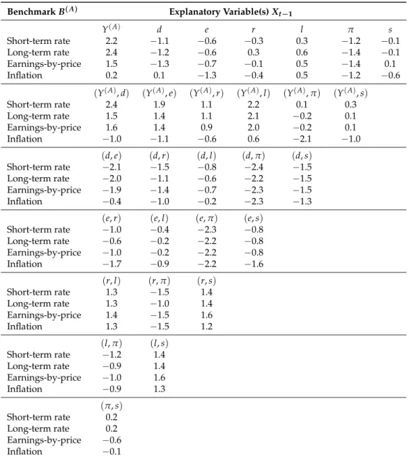
Overall, we find for the one-year horizon that only a few variables have small positive validated
R2V,ν’s and thus possibly some low explanatory power. For example, for the benchmarksB(R),B(L),
andB(E), the excess stock return has the largest validatedR2V,νvalues for one-dimensional models
(2.2%, 2.4%, and 1.5%). This finding would support an ARCH-type variance structure. For the inflation
benchmarkB(C), the model with the long-term interest rate produces the largest validatedR2V,νof
0.5%. When we apply the bootstrap tests introduced in Section2.5, the KNY-test does not reject the
covariate under the benchmarksB(R),B(L)andB(E)at the 5%-level.14 Note that the two-dimensional
models do not add predictive power as the validatedR2V,νvalues remain in the same low range.
Table 2. Predictive power for the variance of one-year excess stock returns Yt(A): the single benchmarking approach. The prediction problem is defined in (2). The same predictive variablesXt−1 are used in the predictions for the conditional mean and variance function. The predictive power (%) is measured byR2V,νas defined in (8). The benchmarksB(A)considered are based on the short-term interest rate (A≡R), long-term interest rate (A≡L), earnings-by-price ratio (A≡E), and consumer price index (A≡C). The predictive variables used areXt−1, given by the dividend-by-price ratiodt−1, earnings-by-price ratioet−1, short-term interest ratert−1, long-term interest ratelt−1, inflationπt−1, term spreadst−1, excess stock returnYt(−A1), or the possible different pairwise combinations as indicated.
BenchmarkB(A) Explanatory Variable(s)X t−1 Y(A) d e r l π s Short-term rate 2.2 −1.1 −0.6 −0.3 0.3 −1.2 −0.1 Long-term rate 2.4 −1.2 −0.6 0.3 0.6 −1.4 −0.1 Earnings-by-price 1.5 −1.3 −0.7 −0.1 0.5 −1.4 0.1 Inflation 0.2 0.1 −1.3 −0.4 0.5 −1.2 −0.6 (Y(A),d) (Y(A),e) (Y(A),r) (Y(A),l) (Y(A),π) (Y(A),s) Short-term rate 2.4 1.9 1.1 2.2 0.1 0.3 Long-term rate 1.5 1.4 1.1 2.1 −0.2 0.1 Earnings-by-price 1.6 1.4 0.9 2.0 −0.2 0.1 Inflation −1.0 −1.1 −0.6 0.6 −2.1 −1.0 (d,e) (d,r) (d,l) (d,π) (d,s) Short-term rate −2.1 −1.5 −0.8 −2.4 −1.5 Long-term rate −2.0 −1.1 −0.6 −2.2 −1.5 Earnings-by-price −1.9 −1.4 −0.7 −2.3 −1.5 Inflation −0.4 −1.0 −0.2 −2.3 −1.3 (e,r) (e,l) (e,π) (e,s) Short-term rate −1.0 −0.4 −2.3 −0.8 Long-term rate −0.6 −0.2 −2.2 −0.8 Earnings-by-price −1.0 −0.2 −2.2 −0.8 Inflation −1.7 −0.9 −2.2 −1.6 (r,l) (r,π) (r,s) Short-term rate 1.3 −1.5 1.4 Long-term rate 1.3 −1.0 1.4 Earnings-by-price 1.4 −1.5 1.6 Inflation 1.3 −1.5 1.2 (l,π) (l,s) Short-term rate −1.2 1.4 Long-term rate −0.9 1.4 Earnings-by-price −1.0 1.6 Inflation −0.9 1.3 (π,s) Short-term rate 0.2 Long-term rate 0.2 Earnings-by-price −0.6 Inflation −0.1
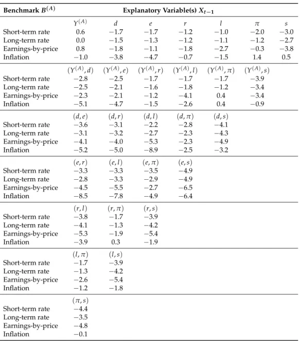
Contrary to the mean prediction, whereKyriakou et al.(2019b) find that five-year predictability
improves over the one-year case, we observe that the majority of predictor based volatility models do
14 The tests were conducted with 1000 repetitions at the 5% significance level for a selected number of cases. We do not present
not surpass the constant volatility alternative for the five-year horizon. Even though some models
produce small positiveR2V,νvalues, this time both the SNS- and the KNY-test do not reject the null of
no predictability. Note that our results are in line withChristoffersen and Diebold(2000) who conclude
that volatility forecastability may be much less important at longer horizons.
Table 3.Predictive power for the variance of five-year excess stock returnsZ(tA): the single benchmarking approach. The prediction problem is defined in (5). The same predictive variablesXt−1are used in the predictions for the conditional mean and variance function. Additional notes: see Table2.
BenchmarkB(A) Explanatory Variable(s)Xt−1
Y(A) d e r l π s Short-term rate 0.6 −1.7 −1.7 −1.2 −1.0 −2.0 −3.0 Long-term rate 0.0 −1.5 −1.3 −1.2 −1.1 −1.2 −2.7 Earnings-by-price 0.8 −1.8 −1.1 −1.8 −2.7 −0.3 −3.8 Inflation −1.0 −3.8 −4.7 −0.7 −1.5 1.4 0.5 (Y(A),d) (Y(A),e) (Y(A),r) (Y(A),l) (Y(A), π) (Y(A),s) Short-term rate −2.8 −2.5 −1.7 −1.7 −1.7 −3.9 Long-term rate −2.5 −2.1 −1.6 −1.8 −1.2 −3.4 Earnings-by-price −2.3 −2.1 −1.2 −4.1 0.4 −3.4 Inflation −5.1 −4.7 −1.5 −2.6 0.4 −0.9 (d,e) (d,r) (d,l) (d,π) (d,s) Short-term rate −3.6 −3.1 −2.2 −2.8 −4.1 Long-term rate −3.1 −3.2 −2.7 −2.3 −4.3 Earnings-by-price −4.1 −4.0 −5.3 −2.3 −4.9 Inflation −5.2 −5.0 −8.9 −2.5 −3.2 (e,r) (e,l) (e,π) (e,s) Short-term rate −3.3 −3.3 −3.5 −4.9 Long-term rate −2.8 −3.3 −2.9 −4.9 Earnings-by-price −4.5 −5.5 −2.7 −6.5 Inflation −8.5 −7.8 −4.9 −6.4 (r,l) (r,π) (r,s) Short-term rate −3.8 −1.7 −3.9 Long-term rate −4.1 −1.3 −4.2 Earnings-by-price −5.3 −1.9 −5.4 Inflation −3.9 0.3 −1.9 (l,π) (l,s) Short-term rate −1.7 −3.9 Long-term rate −1.3 −4.2 Earnings-by-price −2.6 −5.4 Inflation −1.2 −1.8 (π,s) Short-term rate −4.4 Long-term rate −3.5 Earnings-by-price −4.8 Inflation −0.1
3.3. Full Benchmarking Approach
In the next step, we consider the double benchmarking approach ofKyriakou et al.(2019a,2019b)
to analyze now whether transforming the explanatory variables can improve the predictions for the volatility function. Recall that fully nonparametric models suffer in general by the curse of dimensionality. Problems with sparsely distributed annual observations in higher dimensions, as in our framework, could be reduced or circumvented by importing more structure in the estimation process.
Here, we extend the study presented in Section 3.2 transforming both the dependent and independent variables according to the same benchmark. To this end, in our full (double) benchmarking approach, the prediction problems are reformulated as
Yt(A)=m(X(t−A1)) +ν(Xt(−A1))1/2ζt, (14)
Z(tA)=m(X(t−A1)) +ν(Xt(−A1))1/2ωt, (15)
where we use transformed predictive variables
X(t−A1)= 1+Xt−1 B(t−A1) , X∈ {d,e,r,l,π} st−1 B(t−A1) = lt−1−rt−1 B(t−A)1 Yt(−A1) , A∈ {R,L,E,C}. (16)
This approach can be interpreted as a simple way of reducing the dimensionality of the estimation
procedure. The adjusted variableXt(−A1)includes now an additional predictive variable, the benchmark
itself. Results of this empirical study are presented for the one-year horizon in Table4and for the
five-year horizon in Table5.
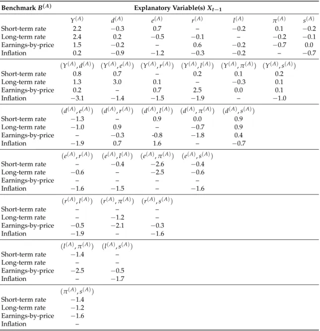
We find that, in comparison to the single-benchmarking approach in the one-year case, the double benchmarking improves in 15 out of 82 models (in the sense of producing a positive and higher
R2V,νas before). However, predictability is still questionable. The best model under the long-term
interest rate benchmarkB(L)uses the pair(Yt(−L)1,e(t−L)1)and yieldsR2V,ν =3.0, while the best model
underB(E)uses the pair(Yt(−E1),lt(−E)1)and yieldsR2V,ν=2.5. The SNS-test rejects for both the null of no
predictability, while the KNY-test does not. For the rest of the new combinations of predictive variables in all benchmarks, both tests again do not reject.
For the five-year case, we find that in comparison to the single-benchmarking the double
benchmarking improves in 11 out of 82 models. The best model underB(E) usesd(t−E)1and yields
RV2,ν=1.8, while underB(C)the covariatesdt(−C)1andlt(−C)1both yieldR2V,ν=1.6. Nevertheless, we do
Table 4.Predictive power for the variance of one-year excess stock returnsYt(A): the double benchmarking approach. The prediction problem is defined in (14). The same predictive variablesXt(−A1)are used in the predictions for the conditional mean and variance. The predictive power (%) is measured byR2
V,ν as defined in (8). The benchmarksB(A)considered are based on the short-term interest rate (A≡R), long-term interest rate (A≡L), earnings-by-price ratio (A≡E), and consumer price index (A≡C). The predictive variables used areX(t−A1)using the indicated benchmarkBt(−A1) as shown in (16). Xt−1 are given by the dividend-by-price ratiodt−1, earnings-by-price ratioet−1, short-term interest rate rt−1, long-term interest ratelt−1, inflationπt−1, term spreadst−1, excess stock returnYt(−A1), or the possible different pairwise combinations as indicated. “–” are not applicable cases of matched covariate with benchmark. Note: s(R) andl(R) (and their combinations withY,d,e,π) have the sameR2V by construction of the transformed spread according to (16). For example,s(t−R)1 = (lt−1−rt−1)/B(t−R)1 =
(1+lt−1)/(1+rt−1)−1 andlt(−R)1= (1+lt−1)/(1+rt−1). The case ofs(L)andr(L)is similar.
BenchmarkB(A) Explanatory Variable(s)X t−1 Y(A) d(A) e(A) r(A) l(A) π(A) s(A) Short-term rate 2.2 −0.3 0.7 – −0.2 0.1 −0.2 Long-term rate 2.4 0.2 −0.5 −0.1 – −0.2 −0.1 Earnings-by-price 1.5 −0.2 – 0.6 −0.2 −0.7 0.0 Inflation 0.2 −0.9 −1.2 −0.3 −0.2 – −0.7 (Y(A),d(A)) (Y(A),e(A)) (Y(A),r(A)) (Y(A),l(A)) (Y(A),π(A)) (Y(A),s(A)) Short-term rate 0.8 0.7 – 0.2 0.1 0.2 Long-term rate 1.3 3.0 0.1 – −0.3 0.1 Earnings-by-price 0.2 – 0.7 2.5 0.0 0.1 Inflation −3.1 −1.4 −1.5 −1.9 – −1.0 (d(A),e(A)) (d(A),r(A)) (d(A),l(A)) (d(A),π(A)) (d(A),s(A)) Short-term rate −1.3 – 0.9 0.0 0.9 Long-term rate −1.0 0.9 – −0.7 0.9 Earnings-by-price – −0.3 -0.8 −1.8 0.4 Inflation −1.9 0.7 1.6 – −0.7 (e(A),r(A)) (e(A),l(A)) (e(A), π(A)) (e(A),s(A)) Short-term rate – −0.4 −2.6 −0.4 Long-term rate −0.6 – −2.5 −0.6 Earnings-by-price – – – – Inflation −1.6 −1.5 – −1.6 (r(A),l(A)) (r(A),π(A)) (r(A),s(A)) Short-term rate – – – Long-term rate – −1.2 – Earnings-by-price −0.5 −2.1 −0.3 Inflation −1.9 – −1.6 (l(A),π(A)) (l(A),s(A)) Short-term rate −1.4 – Long-term rate – – Earnings-by-price −2.5 −0.5 Inflation – −1.7 (π(A),s(A)) Short-term rate −1.4 Long-term rate −1.2 Earnings-by-price −1.6 Inflation –
Table 5. Predictive power for the variance of five-year excess stock returns Zt(A): the double benchmarking approach. The prediction problem is defined in (15). The same predictive variablesX(t−A1) are used in the predictions for the conditional mean and variance. Additional notes: see Table4.
BenchmarkB(A) Explanatory Variable(s)X t−1 Y(A) d(A) e(A) r(A) l(A) π(A) s(A) Short-term rate 0.6 −2.2 −3.2 – −3.1 −3.2 −3.1 Long-term rate 0.0 −3.4 −2.8 −2.8 – −1.3 −2.8 Earnings-by-price 0.8 1.8 – −2.3 −3.2 0.6 −3.8 Inflation −1.0 1.6 0.3 0.6 1.6 – 0.3 (Y(A),d(A)) (Y(A),e(A)) (Y(A),r(A)) (Y(A),l(A)) (Y(A),π(A)) (Y(A),s(A)) Short-term rate −2.1 −4.3 – −4.0 −1.2 −4.0 Long-term rate −3.8 −3.2 −3.6 – −1.1 −3.6 Earnings-by-price 1.1 – −2.8 −3.8 −0.5 −3.4 Inflation 0.3 −0.8 −0.3 0.4 – −1.0 (d(A),e(A)) (d(A),r(A)) (d(A),l(A)) (d(A), π(A)) (d(A),s(A)) Short-term rate −3.7 – −5.4 −2.1 −5.4 Long-term rate −4.2 −5.8 – −3.3 −5.8 Earnings-by-price – −0.4 −2.6 0.3 −3.3 Inflation −4.3 −0.2 −0.8 – −0.8 (e(A),r(A)) (e(A),l(A)) (e(A),π(A)) (e(A),s(A)) Short-term rate – −5.9 −4.9 −5.9 Long-term rate −6.1 – −4.1 −6.1 Earnings-by-price – – – – Inflation −4.8 −4.1 – −2.1 (r(A),l(A)) (r(A),π(A)) (r(A),s(A)) Short-term rate – – – Long-term rate – −2.3 – Earnings-by-price −6.3 −3.2 −6.1 Inflation −1.0 – 0.5 (l(A),π(A)) (l(A),s(A)) Short-term rate −3.4 – Long-term rate – – Earnings-by-price −3.6 −6.2 Inflation – 0.5 (π(A),s(A)) Short-term rate −3.4 Long-term rate −2.3 Earnings-by-price −4.6 Inflation –
3.4. Real-Income Long-Term Pension Prediction
In long-term pension planning or other asset allocation problems optimized with regard to
real-income protection (Gerrard et al.(2019a,2019b); (Merton 2014)), the econometric models should
reflect those needs and use covariates net-of-inflation. Therefore, we take the inflation benchmark
B(C)and analyse in more detail the best model found byKyriakou et al.(2019b), which uses the
earnings-by-price variable for the mean prediction and produced a R2V,m = 12.2 for the one-year
horizon andR2V,m = 12.4 for the five-year horizon (seeKyriakou et al. 2019b, Tables 4 and 5) in
covariates that best predicts the conditional variance.15,16 The empirical findings in terms ofR2V,ν
are shown for the one-year horizon in Table6and the five-year horizon in Table7. For the one-year
horizon, we find in the double benchmarking approach when inflation is the benchmark,B(C)that
the dividend-by-priced(C)together with the short-term interest-rater(C)or the long-term interest-rate
l(C)are chosen as best predictive variables in terms ofR2V,ν(2.9% and 2.0%). Note that these values
are rather low and that the SNS-test does reject the null of no predictability for both models, while the KNY-test does not reject. For all other combinations and also the five-year case, we do not find evidence for statistical significant predictability of the conditional variance. Therefore, we conclude that the constant volatility model is appropriate for practical purposes.
Note further that the ratio in our validation criterion for the mean prediction, R2
V,m, in (8)
compares the sample variance of the estimated residuals from our model based on earnings-by-price (the numerator) with the sample variance of the benchmarked stock returns (the denominator). For
the one-year case, we find from Table1the latter to be equal to 0.18052=0.03258. A simple calculation
using the correspondingRV,m = 12.2% leads then to 0.03258(1−0.122) = 0.02861 or a standard
deviation of 16.91% for returns based on the earnings-model. This means that the linear expression of
real stock returns in terms of real earnings-by-price presented inKyriakou et al.(2019b) as
Real one-year stock return=0.004875+1.119×real earnings-by-price (17)
gives on average 2.4% higher returns at the same risk as the historical mean ¯Y(C).17 Similarly, for the
five-year case, we get from Table1that 0.36422 = 0.1326. From theRV,m = 12.4%, we obtain then
0.1326(1−0.122) =0.1162 or a standard deviation of 34.08% for returns based on the earnings-model.
Thus, the linear expression of real stock returns in terms of real earnings-by-price presented in
Kyriakou et al.(2019b) as
Real five-year stock return=0.2068+2.264×real earnings-by-price (18)
gives on average 6.1% higher returns at the same risk as the historical mean ¯Y(C).18Figure1shows the
estimated nonparametric function ˆm(red solid line) for the one-year horizon (left) and the five-year
horizon (right) under the double inflation benchmark for the earnings-by-price covariate together
with the corresponding historical mean (dashed green line). Figure2depicts histograms and a kernel
density estimate (red solid line) of the standardized predicted returns for the one-year horizon (left) and the five-year horizon (right). The similarity for both horizons is striking and driven by the fact that
the ratio of the slope of the regression lines in (17) and (18) with the corresponding standard deviation
given above yields almost the same value of 6.63.
15 Note that until now we have used the same set of covariates in both steps of our analysis to reduce the overwhelming
number of models. It is also clear that not all combinations of variables are practically relevant. Now, we relax this restriction for the model with the highest predictive power for the returns.
16 Tables6and7also present the results for the short- and long-term interest benchmarksB(R)
andB(L). However, it is again
hard to find predictability at all in these cases. Note that the benchmark using the earnings-by-price variableB(E)is not
applicable since it matches the covariate and the benchmark in the first step.
17 Here, we use the Sharpe-ratio for the comparison. From Table1, we get ¯Y(C)=
6.41% and divide it either by 18.05% or by 16.91%. We obtain 0.355 and 0.379, which corresponds to a difference of 2.4% points.
18 Here, we use again the Sharpe-ratio for the comparison. From Table1, we get ¯Y(C)=
32.34% and divide it either by 36.42% or by 34.08%. We obtain 0.888 and 0.949, which corresponds to a difference of 6.1% points.
Finally, we consider a simple mean-reverting autoregressive model of order one for the real
earnings-by-price—the main drivers of real returns in Equations (17) and (18)—and estimate it
with ordinary least squares (OLS)19:
Change in real earnings-by-price
=−0.715×(real earnings-by-price−mean of real earnings-by-price). (19)
Note that, for the whole sample period (1872–2019), the mean and standard deviation of real earnings-by-price are 0.0524 and 0.0595, resp. Moreover, using the current (30/09/2019) value of
real earnings-by-price of 0.0278, model (19) predicts a change in real earnings-by-price of 0.0176,
i.e., an expected value of real earnings-by-price of 0.0454 for 2020Q3, which is still below the
long-term average.20
We subsequently calculate the correlation between the estimated residuals of models (17) and (19)
to be −0.014. A standard stationary block-bootstrap (Politis and Romano 1994) based on 10,000
repetitions and a block-length of 12 suggests that this correlation is not statistically significantly different from zero. The correlation structure between returns and their drivers is important while
searching for optimal investment strategies in a dynamic market, see Kim and Omberg (1996).
Gerrard et al.(2019c) follow the approach ofKim and Omberg(1996) in a long-term return setting and show that the above correlation is very hard to estimate with precision. Sometimes, it is negative and, with a slight change of data, it is positive, and a test would almost always provide that zero correlation cannot be rejected. When this added insight is provided that zero correlation significantly simplifies that technical calculation of the optimal dynamic strategy while significantly reducing parameter uncertainty, the conclusion seems clear: we should work with zero correlation unless there is a strong argument not to do that. In our case—which is a discrete analogue to the continuous models considered inGerrard et al.(2019c) andKim and Omberg(1996)—it is, therefore, comforting that we can provide a simple zero-correlation econometric model to guide the market dynamics. In further work, we expect the simple econometric model of this paper to be used while generalizing the non-dynamic new
approach to pension products ofGerrard et al.(2019a,2019b).
19 The estimated coefficient is significant at the 0.1%-level (with a corresponding standard error of 0.08), the residual standard
error of the regression is 0.0572, and itsR2has a value of 0.357.
20 The following values are used for the calculation of the current real earnings-by-price: P = 2976.74,E = 135.53,
Table 6. Predictive power for the variance of one-year excess stock returns Yt(A): the double benchmarking approach for the conditional mean model with earnings-by price as single covariate. The prediction problem is defined in (14). The predictive power (%) is measured byR2V,νas defined in (8). The benchmarksB(A)considered are based on the short-term interest rate (A≡R), long-term interest rate (A ≡ L), and consumer price index (A ≡ C). The predictive variables used areX(t−A1) using the indicated benchmarkB(t−A1)as shown in (16).Xt−1are given by the dividend-by-price ratio dt−1, earnings-by-price ratioet−1, short-term interest ratert−1, long-term interest ratelt−1, inflation πt−1, term spreadst−1, excess stock returnYt(−A1), or the possible different pairwise combinations as indicated. “–” are not applicable cases of matched covariate with benchmark. Note: s(R) and l(R)(and their combinations withY,d,e,π) have the sameR2V,νby construction of the transformed spread according to (16). For example,s(t−R)1 = (lt−1−rt−1)/Bt(−R)1 = (1+lt−1)/(1+rt−1)−1 and l(t−R)1= (1+lt−1)/(1+rt−1). Similar is the case ofs(L)andr(L).
BenchmarkB(A) Explanatory Variable(s)Xt−1
Y(A) d(A) e(A) r(A) l(A) π(A) s(A) Short-term rate 1.0 0.3 0.7 – 0.1 −0.4 0.1 Long-term rate 1.4 0.1 −0.5 0.9 – −0.1 0.9 Inflation 0.4 −0.6 −1.2 −0.4 −0.1 – 0.8 (Y(A),d(A)) (Y(A),e(A)) (Y(A),r(A)) (Y(A),l(A)) (Y(A), π(A)) (Y(A),s(A)) Short-term rate 0.6 0.7 – 0.2 −0.5 0.2 Long-term rate 0.7 2.0 0.7 – −0.6 0.7 Inflation −1.7 −1.6 −1.5 −1.7 – −0.4 (d(A),e(A)) (d(A),r(A)) (d(A),l(A)) (d(A),π(A)) (d(A),s(A)) Short-term rate 0.0 – −0.5 −0.4 −0.5 Long-term rate −1.0 0.3 – −1.4 0.3 Inflation −1.9 2.9 2.0 – 1.5 (e(A),r(A)) (e(A),l(A)) (e(A),π(A)) (e(A),s(A)) Short-term rate – 0.5 −2.2 0.5 Long-term rate −0.7 – −2.5 −0.7 Inflation −0.9 −1.7 – −0.3 (r(A),l(A)) (r(A),π(A)) (r(A),s(A)) Short-term rate – – – Long-term rate – −0.4 – Inflation −0.5 – 0.7 (l(A),π(A)) (l(A),s(A)) Short-term rate 0.1 – Long-term rate – – Inflation – −0.2 (π(A),s(A)) Short-term rate 0.1 Long-term rate −0.4 Inflation –
Table 7. Predictive power for the variance of five-year excess stock returns Zt(A): the double benchmarking approach for the conditional mean model with earnings-by price as single covariate. The prediction problem is defined in (15). Additional notes: see Table6.
BenchmarkB(A) Explanatory Variable(s)X t−1 Y(A) d(A) e(A) r(A) l(A) π(A) s(A) Short-term rate 0.1 −1.8 −3.2 – −4.5 −2.5 −4.5 Long-term rate 0.6 −3.9 −2.8 −4.2 – −1.1 −4.2 Inflation 0.0 −0.1 0.3 −0.4 −0.1 – −2.6 (Y(A),d(A)) (Y(A),e(A)) (Y(A),r(A)) (Y(A),l(A)) (Y(A),π(A)) (Y(A),s(A)) Short-term rate −1.7 −4.6 – −5.7 −3.7 −5.7 Long-term rate −4.5 −4.5 −4.2 – −2.5 −4.2 Inflation −1.9 −1.8 −1.9 −1.7 – −3.9 (d(A),e(A)) (d(A),r(A)) (d(A),l(A)) (d(A), π(A)) (d(A),s(A)) Short-term rate −6.2 – −7.1 −4.3 −7.1 Long-term rate −4.5 −7.9 – −5.2 −7.9 Inflation −3.9 −2.1 −3.2 – −2.8 (e(A),r(A)) (e(A),l(A)) (e(A),π(A)) (e(A),s(A)) Short-term rate – −8.1 −5.8 −8.1 Long-term rate −6.6 – −4.9 −6.6 Inflation −2.8 −3.4 – −2.6 (r(A),l(A)) (r(A),π(A)) (r(A),s(A)) Short-term rate – – – Long-term rate – −5.7 – Inflation −3.0 – −3.1 (l(A),π(A)) (l(A),s(A)) Short-term rate −6.5 – Long-term rate – – Inflation – −3.0 (π(A),s(A)) Short-term rate −6.5 Long-term rate −5.7 Inflation – ● ● ● ● ● ● ● ● ● ● ● ● ● ● ● ● ● ● ● ● ● ● ● ● ● ● ● ● ● ● ● ● ● ● ● ● ● ● ● ● ● ● ● ● ● ● ● ● ● ● ● ● ● ● ● ● ● ● ● ● ● ● ● ● ● ● ● ● ● ● ● ● ● ● ● ● ● ● ● ● ● ● ● ● ● ● ●● ● ● ● ● ● ● ● ● ● ● ● ● ● ● ● ● ● ● ● ● ● ● ● ● ● ● ● ● ● ● ● ● ● ● ● ● ● ● ● ● ● ● ● ● ● ● ● ● ● ● ● ● ● ● ● ● ● ● −0.1 0.0 0.1 0.2 0.3 −0.4 −0.2 0.0 0.2 0.4 earnings one−y ear e
xcess stock retur
n nonpar hist. avg ● ● ● ● ● ● ● ● ● ● ● ● ● ● ● ● ● ● ● ● ● ● ● ● ● ● ● ● ● ● ● ● ● ● ● ● ● ● ● ● ● ● ● ● ● ● ● ● ● ● ● ● ● ● ● ● ● ● ● ● ● ● ● ● ● ● ● ● ● ● ● ● ● ● ● ● ● ● ● ● ● ● ● ● ● ● ● ● ● ● ● ● ● ● ● ● ● ● ● ● ● ● ● ● ● ● ● ● ● ● ● ● ● ● ● ● ● ● ●● ● ● ● ● ● ● ● ● ● ● ● ● ● ● ● ● ● ● ● ● ● ● −0.1 0.0 0.1 0.2 0.3 −0.5 0.0 0.5 1.0 earnings fiv e−y ear e
xcess stock retur
n
nonpar hist. avg
Figure 1.Double inflation benchmark. Relation between real stock returns and real earnings-by-price. Estimated nonparametric function ˆm (red solid line) and historical average (dashed green line).
standardized predicted one−year excess stock return Density −1.0 −0.5 0.0 0.5 1.0 1.5 0.0 0.5 1.0 1.5 density estimate normal distribution
standardized predicted five−year excess stock return
Density −1.0 −0.5 0.0 0.5 1.0 1.5 0.0 0.5 1.0 1.5 density estimate normal distribution
Figure 2.Standardized predicted stock returns in excess of the inflation benchmark (based on the model using earnings-by-price as covariate for mean-prediction; double benchmarking). Histogram, kernel density estimate (red), and fitted normal distribution (green).Left: one-year horizon.Right: five-year horizon. Period: 1872–2019. Data: annual S&P 500.
4. Conclusions
In this paper, we extend the original working framework ofKyriakou et al.(2019a,2019b) of
forecasting stock returns to modelling their conditional variance and test for predictability in this context. We consider returns of one-year and five-year horizons in excess of different benchmarks, considering the short- and long-term rate, the earnings-by-price ratio, and the inflation rate. We use popular explanatory variables with predictive power such as the dividend-by-price ratio, the earnings-by-price ratio, the short- and long-term interest rates, the term spread, the inflation rate, as well as the lagged excess stock return, in one- and two-dimensional settings, with the returns benchmarked or also the covariates used to predict them.
In our analysis, we find only little to no evidence of model-based volatility predictability for the one-year and five-year horizon. Only for a few of the models considered under different benchmarks, we get validation measures that are positive and significantly different from zero but of a rather small magnitude. We thus conclude that volatility forecastability is much less important at longer horizons regardless of the chosen combination of explanatory variables. The homoscedastic historical average of the squared return prediction errors gives an adequate approximation of the unobserved realised conditional variance for both the one-year and five-year horizon.
In the practically important double inflation benchmarking case, we find that the model with the largest predictive power is not only of linear functional form based on real earnings-by-price but also has a constant variance for both horizons. A simple mean-reverting linear AR1-model for the real-earnings-by-price allows then to analyse the correlation structure between returns and their main drivers. We find zero correlation which significantly simplifies the econometric modelling to guide market dynamics. This is an important observation and a relatively simple starting point when constructing forecasting models for real-value pension prognoses for long-term saving strategies.
Author Contributions:All authors contributed equally to this work.
Funding:The authors thank: (i) the Institute and Faculty of Actuaries in the UK for funding this research through the grant “Minimizing Longevity and Investment Risk while Optimizing Future Pension Plans”, and (ii) the University of Graz for the Open Access Funding.
Conflicts of Interest:The authors declare no conflict of interest.
References
Andersen, Torben G., Tim Bollerslev, Francis X. Diebold, and Heiko Ebens. 2001. The distribution of realized stock return volatility. Journal of Finacial Economics61: 43–76. [CrossRef]
Burman, Prabir, Edmond Chow, and Deborah Nolan. 1994. A cross-validatory method for dependent data.
Biometrika81: 351–58. [CrossRef]
Chen, Qingqing, and Yongmiao Hong. 2010. Predictability of Equity Returns Over Different Time Horizons:
A Nonparametric Approach. Working Paper. Ithaca: Cornell University/Department of Economics.
Cheng, Tingting, Jiti Gao, and Oliver Linton. 2019. Nonparametric Predictive Regressions for Stock Return Predictions. Cambridge Working Papers in Economics: 1932. Cambridge: Faculty of Economics, University of Cambridge. Christoffersen, Peter F., and Francis X. Diebold. 2000. How relevant is volatility forecasting for financial risk
management?Review of Economics and Statistics82: 12–22. [CrossRef]
Chu, C. K., and J. S. Marron. 1991. Comparison of two bandwidth selectors with dependent errors. The Annals of
Statistics19: 1906–18. [CrossRef]
De Brabanter, Kris, Jos De Brabanter, Johan A.K. Suykens, and Bart De Moor. 2011. Kernel regression in the presence of correlated errors. Journal of Machine Learning Research12: 1955–76.
Fan, Jianqing, and Qiwei Yao. 1998. Efficient estimation of conditional variance functions in stochastic regression.
Biometrika85: 645–60. [CrossRef]
Galbraith, John W. 2003. Content horizons for univariate time-series forecasts. International Journal of Forecasting 19: 43–55. [CrossRef]
Galbraith, John W., and Turgut Kisinbay. 2005. Content horizons for conditional variance forecasts. International
Journal of Forecasting21: 249–60. [CrossRef]
Geller, Juliane, and Michael H. Neumann. 2018. Improved local polynomial estimation in time series regression.
Journal of Nonparametric Statistics30: 1–27. [CrossRef]
Gerrard, Russell, Munir Hiabu, Ioannis Kyriakou, and Jens Perch Nielsen. 2019a. Communication and personal selection of pension saver’s financial risk.European Journal of Operational Research274: 1102–11. [CrossRef] Gerrard, Russell, Munir Hiabu, Ioannis Kyriakou, and Jens Perch Nielsen. 2019b. Self-selection and risk sharing
in a modern world of life-long annuities. British Actuarial Journal23: e30. [CrossRef]
Gerrard, Russell, Munir Hiabu, Jens Perch Nielsen, and Peter Vodicka. 2019c. Long-Term Real Dynamic Investment
Planning. Working Paper. London: Cass Business School.
Geweke, John F. 1996. Monte carlo simulation and numerical integration. InHandbook of Computational Economics. Edited by Hans M. Amman, David A. Kendrick and John Rust. Amsterdam: Elsevier, vol. I, pp. 731–800. Glad, Ingrid K. 1998. Parametrically guided non-parametric regression. Scandinavian Journal of Statistics25: 649–68.
[CrossRef]
Gonzales-Manteiga, Wenceslao, and Rosa M. Crujeiras. 2013. An updated review of goodness-of-fit tests for regression models. Test22: 361–411. [CrossRef]
Härdle, Wolfgang K., and Enno Mammen. 1993. Comparing nonparametric versus parametric regression fits.
Annals of Statistics21: 1926–47. [CrossRef]
Härdle, Wolfgang K., and Alexandre B. Tsybakov. 1997. Local polynomial estimators of the volatility function in nonparametric autoregression. Journal of Econometrics81: 223–42. [CrossRef]
Kim, Tong Suk, and Edward Omberg. 1996. Dynamic nonmyopic portfolio behavior. The Review of Financial
Studies9: 141–61. [CrossRef]
Kothari, S. P., Jonathan Lewellen, and Jerold B. Warner. 2006. Stock returns, aggregate earnings surprises, and behavioral finance. Journal of Financial Economics79: 537–68. [CrossRef]
Kreiss, Jens-Peter, Michael H. Neumann, and Qiwei Yao. 2008. Bootstrap tests for simple structures in nonparametric time series regression. Statistics and Its Interfaces1: 367–80. [CrossRef]