A fixed-point algorithm for blind source separation with nonlinear autocorrelation

(1)

Contents lists available atScienceDirect

Journal of Computational and Applied

Mathematics

journal homepage:www.elsevier.com/locate/cam

A fixed-point algorithm for blind source separation with nonlinear

autocorrelation

I

Zhenwei Shi

∗

_{, Zhiguo Jiang, Fugen Zhou}

Image Processing Center, School of Astronautics, Beijing University of Aeronautics and Astronautics, Beijing 100083, PR China

a r t i c l e i n f o

Article history:

Received 8 December 2007

Received in revised form 8 March 2008 Keywords:

Blind source separation (BSS) Independent component analysis (ICA) Nonlinear autocorrelation

Fixed-point algorithm

a b s t r a c t

This paper addresses blind source separation (BSS) problem when source signals have the temporal structure with nonlinear autocorrelation. Using the temporal characteristics of sources, we develop an objective function based on the nonlinear autocorrelation of sources. Maximizing the objective function, we propose a fixed-point source separation algorithm. Furthermore, we give some mathematical properties of the algorithm. Computer simulations for sources with square temporal autocorrelation and the real-world applications in the analysis of the magnetoencephalographic recordings (MEG) illustrate the efficiency of the proposed approach. Thus, the presented BSS algorithm, which is based on the nonlinear measure of temporal autocorrelation, provides a novel statistical property to perform BSS.

1. Introduction

Recently, blind source separation (BSS) [6,11], as an increasingly popular data analysis technique, has received wide attention in various fields such as biomedical signal processing and analysis, speech and image processing, wireless telecommunication systems, data mining, etc. The main task of BSS is to recover original sources from their mixtures using some statistical properties of original sources.

The blind source separation problem has been studied by researchers in applied mathematics, neural networks and statistical signal processing. Several methods for BSS using the statistical properties of original sources have been proposed, such as non-Gaussianity (or equivalently, independent component analysis, ICA) [1,3,5–8,11–13,24,

34], linear predictability or smoothness [2,6], linear autocorrelation [4,19,31], coding complexity [9,26,27,29], temporal predictability [23], nonstationarity [10,18,21], sparsity [14,15,25,35], energy predictability [28], nonlinear innovation [30] and nonnegativity [20,22], etc.

In this paper, we present a way using nonlinear autocorrelation of source signals for BSS. We propose a fixed-point algo-rithm for BSS based on nonlinear autocorrelation and analyze its stability conditions. We show that the BSS problem can be solved by maximizing nonlinear temporal autocorrelation of the sources. When sources have square temporal autocorrela-tion, we demonstrate that the efficient implementation of the method. Also, the proposed algorithm can extract the most in-teresting and meaningful sources in brain magnetoencephalography (MEG) data analysis. Thus, the presented BSS algorithm, which is based on the nonlinear measure of temporal autocorrelation, provides a new statistical property to perform BSS.

The structure of the paper is as follows. The objective function based on the nonlinear autocorrelation of the desired source signals, and a fixed-point algorithm for optimizing the objective function are proposed in Section2. Furthermore, we analyze the stability conditions of the fixed-point algorithm in Section3. In Section4, experiments on different datasets are presented. Some conclusions are drawn in Section5.

I_{The work was supported by the National Science Foundation of China (60605002, 60776793, 10571018).}

∗_{Corresponding author. Tel.: +86 10 627 96 872; fax: +86 10 627 86 911.} E-mail address:[email protected](Z. Shi).

(2)

2. Proposed algorithm 2.1. Objective function

We observe sensor signalsx

(

t

)

=

(

x1

(

t

), . . . ,

xn

(

t

))

Tdescribed in the matrix notation:

x

(

t

)

=As

(

t

),

(1)

whereAis ann×nunknown mixing matrix,s

(

t

)

=

(

s1

(

t

), . . . ,

sn

(

t

))

Tis a vector of unknown zero-mean and unit-variance

primary sources.

The basic problem of BSS is then to estimate both the mixing matrixAand the source signalssi

(

t

)

using only observations

of the mixturesxi

(

t

)(

i=1

, . . . ,

n

)

, i.e., to find ann×nseparating matrixW=

(

w1

, . . . ,

wN

)

Tsuch that the unmixed signals

y

(

t

)

=

(

y₁

(

t

), . . . ,

yN

(

t

))

T,

y

(

t

)

=Wx

(

t

)

(2)

are the estimated source signals. The sources are recovered up to scaling and permutation.

A useful preprocessing strategy in BSS is to first whiten the observed variables [11]. This means that we transform the observed vectorxlinearly so that we obtain a new vectorx˜which is white, i.e., its components are uncorrelated and their variances equal unity. In other words,xis linearly transformed into a vector

˜

x

(

t

)

=Vx

(

t

)

=VAs

(

t

)

(3)

whose covariance matrix equals the identity matrix:E{ ˜x

(

t

)

x˜

(

t

)

T_{} =}_I_{, where}_V_{is a whitening matrix.}

If we want to estimate a desired source signal, for this purpose we design a single processing unit described as

˜

yi

(

t

)

=wTix˜

(

t

),

(4)

˜

yi

(

t−

τ

k

)

=wTix˜

(

t−

τ

k

),

(5)

wherewi =

(

wi1

, . . . ,

win

)

Tis the weight vector which corresponds to the estimate of one row of

(

VA

)

−1, andy˜i

(

t

)

is the

output signal which corresponds to the estimate of the source signalsi

(

t

)

, and

τ

kis a certain time delay.

We present the following constrained maximization problem based on several time delay nonlinear autocorrelation function of the desired source:

max kwik=1 Ψ1

(

wi

)

= M X k=1 E{G

(

˜yi

(

t

))

G

(

y˜i

(

t−

τ

k

))

} = M X k=1 E{G

(

wT ix˜

(

t

))

G

(

w T ix˜

(

t−

τ

k

))

}

.

(6)

Gis a differentiable nonlinear function, which measures the nonlinear autocorrelation degree of the desired source. Examples of choices areG

(

u

)

=u2orG

(

u

)

=log cosh

(

u

)

.

Sometimes, we could use only one time lagged nonlinear autocorrelation to obtain the desired source signal: max

kwik=1

Ψ2

(

wi

)

=E{G

(

y˜i

(

t

))

G

(

y˜i

(

t−

τ

k

))

}

=E{G

(

wT_ix˜

(

t

))

G

(

wT_ix˜

(

t−

τ

k

))

}

.

(7)

Thus, the constrained maximization problem(7)is a special case of the problem(6)when only one time delay can be used. In Section3, we give some theoretical properties about the maximization problems(6)and(7).

2.2. Learning algorithms

Maximizing the objective function in(6), we derive a fixed-point blind source separation (BSS) algorithm. The gradient ofΨ1

(

wi

)

with respect towican be obtained as

∂

Ψ1

(

wi

)

∂

wi = M X k=1 E{g

(

˜yi

(

t

))

G

(

y˜i

(

t−

τ

k

))

x˜

(

t

)

+G

(

y˜i

(

t

))

g

(

y˜i

(

t−

τ

k

))

x˜

(

t−

τ

k

)

}

.

(8)

The functiongis the derivative ofG. According to the Kuhn–Tucker conditions [17], we note that at a stable point of the optimization problem(6), the gradient ofΨ1

(

wi

)

atwimust point in the direction ofwi, thus we can optimize the objective

function in(6)by a fixed-point algorithm [11]. This means that we have

wi ← M X k=1 E{g

(

y˜i

(

t

))

G

(

y˜i

(

t−

τ

k

))

x˜

(

t

)

+G

(

y˜i

(

t

))

g

(

y˜i

(

t−

τ

k

))

x˜

(

t−

τ

k

)

}

,

wi ←wi

/

kwik

.

(9)

(3)

If only one time delay can be used, i.e. maximizing the objective function in(7), we have

wi ←E{g

(

y˜i

(

t

))

G

(

y˜i

(

t−

τ

k

))

x˜

(

t

)

+G

(

y˜i

(

t

))

g

(

y˜i

(

t−

τ

k

))

x˜

(

t−

τ

k

)

}

,

wi ←wi

/

kwik

.

(10)

To estimate several source signals, one can simply use a deflation scheme (Gram-Schmidt orthogonalization scheme) or the symmetric orthogonalization [11].

Thus, the fixed-point BSS algorithm (FixNA- BSS using the Fixed-point algorithm for maximizing the Nonlinear

Autocorrelation) is obtained as follows:

Algorithm outline: FixNA (estimating one source)

(1) Center the data to make its mean zero and whiten the data to givex˜

(

t

)

. Choose random initial values forwi,

τ

k, andM.

(2) Update the weight vector by

wi ← M X k=1 E{g

(

y˜i

(

t

))

G

(

˜yi

(

t−

τ

k

))

x˜

(

t

)

+G

(

y˜i

(

t

))

g

(

y˜i

(

t−

τ

k

))

x˜

(

t−

τ

k

)

}

,

wi ←wi

/

kwik

.

(11)

(3) If not converged, go back to step (2).

Note that convergence of the fixed-point algorithm means that the old and new values ofwipoint in the same direction, as

the well-know fixed-point ICA algorithms [8,11].

To estimate the separating matrixW=

(

w1

, . . . ,

wn

)

Tor estimate all the source signals, one can simply use a deflation

scheme (one-by-one estimation) or the symmetric orthogonalization [11].

3. Theoretical properties of the FixNA

We analyze the stability conditions about the FixNA in this section.1

Theorem 1. Assume that the input data follows the model(1)with whitened datax˜ =VAswhereVis the whitening matrix, and Ψ1

(

w

)

is a sufficiently smooth even function. Furthermore, assume that{si

,

si,τk}and{sj

,

sj,τk}

(

∀j6=i

)

are mutually independent.

Then the local maxima ofΨ1

(

w

)

under the constraintkwk =1include one row of the inverse of the mixing matrixVAsuch that

the corresponding desired source signalsisatisfy

M X k=1 E{g0

₍

_s i

)

G

(

si,τk

)

+g 0

₍

_s i,τk

)

G

(

si

)

+2sjsj,τkg

(

si

)

g

(

si,τk

)

−sig

(

si

)

G

(

si,τk

)

−siτg

(

si,τk

)

G

(

si

)

}

<

0

, (

∀j6=i

),

(12)

wheregis the derivative ofG, andg0_{is the derivative of}_g_.

Proof. Assume that{si

,

si,τk}and{sj

,

sj,τk}

(

∀j6=i

)

are mutually independent, and the vectorx˜is white, we have:

E{ ˜xx˜T} =VAE{ssT}ATVT=

(

VA

)(

VA

)

T=I

,

(13) which means the matrixVAis orthogonal. Make the change of coordinatesp =

(

p1

, . . . ,

pn

)

T = ATVTwand note that

wT_x_˜₌_wT_VAs_{, we have:} Ψ1

(

p

)

= M X k=1 E{G

(

pT_s

₎

_G

₍

_pT_s τk

)

}

.

(14)

It is enough to analyze the stability of the pointp=e1, wheree1=

(

1

,

0

,

0

, . . .)

T(becauseΨ1

(

w

)

is even, nothing changes

for

(

−1

,

0

,

0

, . . .)

T_{). Evaluating the gradient and the Hessian at point}_p₌_e

1and using the independency assumptions, and

making a small perturbation

ε

=

(

ε

₁

,

ε

₂

, . . .)

T, we obtain:

Ψ1

(

e1+

ε

)

= Ψ1

(

e1

)

+

ε

T

∂

Ψ1

(

e1

)

∂

p + 1 2

ε

T

∂

2Ψ1

(

e1

)

∂

p2

ε

+o

(

k

ε

k 2

₎

= Ψ1

(

e1

)

+ M X k=1 E{s1g

(

s1

)

G

(

s1,τk

)

+s1τg

(

s1,τk

)

G

(

s1

)

}

ε

1 + M X k=1 1 2[E{s 2 1g 0

₍

s1

)

G

(

s1,τk

)

+s 2 1,τkg 0

₍

s1,τk

)

G

(

s1

)

+2s1s1,τkg

(

s1

)

g

(

s1,τk

)

}]

ε

2 1 +1 2 M X k=1 X j>1 [E{g0

(

s1

)

G

(

s1,τk

)

+g 0

₍

s1,τk

)

G

(

s1

)

+2sjsj,τkg

(

s1

)

g

(

s1,τk

)

}

ε

2 j] +o

(

k

ε

k 2

_).

₍₁₅₎

(4)

Due to the constraintkwk = 1 and the matrixVAis orthogonal, we havekpk = kAT_VT_w_{k =} _{1. Thus, we get}

_ε

1 =

q

1−

ε

2₂−

ε

2₃− · · · −1. Due to the fact that√1−

α

=1−α

2+o

(

α

)

, the term of order

ε

2

1iso

(

k

ε

k2

)

, i.e., of higher order, and

can be neglected [11]. Using the first-order approximation for

ε

1, we obtain

ε

1 = −Pj>1

ε2 j 2 +o

(

k

ε

k2

)

[11], which finally gives Ψ1

(

e1+

ε

)

= Ψ1

(

e1

)

+ 1 2 M X k=1 X j>1 E{g0

(

s1

)

G

(

s1,τk

)

+g 0

₍

s1,τk

)

G

(

s1

)

+2sjsj,τkg

(

s1

)

g

(

s1,τk

)

−s1g

(

s1

)

G

(

s1,τk

)

−s1,τkg

(

s1,τk

)

G

(

s1

)

}

ε

2 j +o

(

k

ε

k2

)

(16)

which clearly provesp=e1is an extremum, and of the type implied by the condition of the theorem.

If we choose only one time delay, we can similarly prove the following corollary.

Corollary 1. Assume that the input data follows the model(1)with whitened datax˜ =VAswhereVis the whitening matrix, and Ψ2

(

w

)

is a sufficiently smooth even function. Furthermore, assume that{si

,

si,τk}and{sj

,

sj,τk}

(

∀j6=i

)

are mutually independent.

Then the local maxima ofΨ2

(

w

)

under the constraintkwk =1include one row of the inverse of the mixing matrixVAsuch that

the corresponding desired source signalsisatisfy

E{g0

(

si

)

G

(

si,τk

)

+g 0

₍

si,τk

)

G

(

si

)

+2sjsj,τkg

(

si

)

g

(

si,τk

)

−sig

(

si

)

G

(

si,τk

)

−siτg

(

si,τk

)

G

(

si

)

}

<

0

, (

∀j6=i

),

(17)

wheregis the derivative ofG, andg0_{is the derivative of} _g_.

Remark 1. Assume that the following conditions are satisfied

(

∀j6=i

)

: (a){si

,

si,τk}and{sj

,

sj,τk}are mutually independent;

(b)E{sjsj,τk} =0, from(12), we have the further stability condition:

M X k=1 E{g0

(

si

)

G

(

si,τk

)

+g 0

₍

si,τk

)

G

(

si

)

−sig

(

si

)

G

(

si,τk

)

−si,τkg

(

si,τk

)

G

(

si

)

}

<

0

, (

∀j6=i

).

(18)

Particularly, assume that the square functionG

(

u

)

=u2is chosen, we have the stability conditionPM

k=1cov

(

s2i

,

s2i,τk

)

>

0. Remark 2. Assume that the signal has no time dependencies andG

(

si,τk

)

=1, from the stability condition(17), we obtain:

E{g0

₍

_s

i

)

−sig

(

si

)

}

<

0

.

(19)

This is in fact the well-known stability condition of independent component analysis (ICA) [11].

4. Experimental results

4.1. Experimental results about source signals with square temporal autocorrelations

We demonstrate that when we chooseG

(

u

)

=u2_and_G

₍

_u

₎

₌_log

₍

_cosh

₍

_u

₎₎

_{, the two FixNA algorithms}2_{can separate the}

source signals with square temporal autocorrelations.

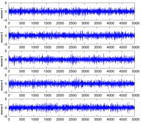
We create five artificial signals which have square temporal autocorrelations as follows (with Gaussian marginal distributions, zero linear autocorrelations)3_[₁₀_{]: first, we create five signals using a first-order autoregressive model with}

constant variances of the innovations, with 5000 time points. The signals are created with Gaussian innovations and have identical autoregressive coefficients (0.8). All these innovations have constant unit variance. Then, the signs of the signals are completely randomized by multiplying each signal by a binary i.i.d. signal that takes the values±1 with equal probabilities. The five source signals are shown inFig. 1. The source signals are mixed with 5×5 random matrices. The FixNA algorithms with the nonlinear functions (G

(

u

)

=u2andG

(

u

)

=log

(

cosh

(

u

))

) with the symmetric orthogonalization are used to estimate the separating matrix. For comparison, we also run the cumulant-based fixed-point approach using the nonstationarity of variance (FPNSV) (

τ

k=1) [10]. In order to measure the accuracy of separation, we calculate the performance index [1,16,

28,30] PI= 1 n2 ( _n X i=1 rPIi+ n X j=1 cPIj ) = 1 n2    n X i=1   n X j=1 |pij| max k |pik| −1  + n X j=1   n X i=1 |pij| max k |pkj| −1     

,

(20)

2 We choose the initial valuesτk=1 andM=1 for the two FixNA algorithms, which are to be suitable for the all experiments.

3 Thus, source signals of this kind could not be separated by ordinary source separation methods based on non-Gaussianity, such as FastICA [11], linear correlation method such as AMUSE [31] and SOBI [4].

(5)

Fig. 1. Five sources with square temporal autocorrelation. whererPIi=Pnj=1 |pij| maxk|pik|−1 andcPIj= Pn i=1 |pij|

maxk|pkj|−1 in whichpijis theijth element ofn×nmatrixP=WVA. The term rPIigives the error of the separation of the output componentyiwith respect to the sources andcPIjmeasures the degree

of the sourcecjappearing multiple times at the output. The larger the valuePIis, the poorer the statistical performance of

a BSS algorithm [1,16,28,30].

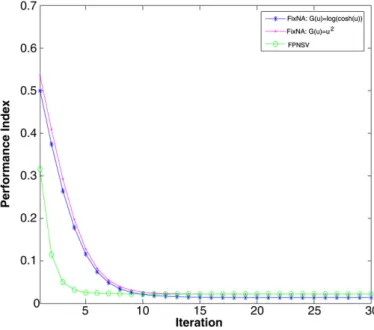
Fig. 2 shows the average performance indexes over 100 independent trials against iteration numbers by the three

algorithms. The FixNA algorithm usingG

(

u

)

=u2performs similarly to the FPNSV algorithm in the sense of the separation accuracy. The FastNA algorithm usingG

(

u

)

=log

(

cosh

(

u

))

has a slightly better performance than the other two algorithms. To investigate the robustness of algorithms, we randomly add 30 outliers whose values are 10 in each source signal.

Fig. 3shows the average performance indexes over 100 independent trials against iteration numbers. Obviously, the FixNA

algorithm usingG

(

u

)

= log

(

cosh

(

u

))

outperforms the two other algorithms when the outliers are introduced. In fact, the FPNSV algorithm and the FixNA algorithm usingG

(

u

)

= u2are both sensitive to the outliers and degrade in performance. Thus, the FixNA algorithm with the nonlinearG

(

u

)

=log

(

cosh

(

u

))

could have better convergence in practice.

4.2. Applications in magnetoencephalography (MEG) data analysis

Magnetoencephalography (MEG) is a passive functional brain imaging technique which, under ideal conditions, can monitor the activation of a neuronal population with a spatial resolution of a few mm and with millisecond temporal resolution. When performing MEG measurements, physicians often have to deal with considerable amounts of artifacts that may render impossible the extraction of valuable information therein. The presence of artifacts, such as eye and muscle activity, the activity of heart and environment electric, digital watch and magnetic disturbances, may render impossible the extraction of useful information from MEG data. If the magnitude of artifacts is larger than that of brain signals, it may become hard to distinguish and interpret the actual and valuable brain activity [32,33]. It is challenging to identify and remove the artifacts from the signals and analyze/explain the brain signals themselves.

Independent component analysis (ICA) has been shown effective to extract and eliminate the artifacts [32,33]. Unlike ICA which assumes that the source signals are non-Gaussian, we use the nonlinear autocorrelation to capture the statistical character of sources. Several artifact structures are evident, such as eye and muscle activity. Thus, the nonlinear temporal autocorrelation is also likely a strong feature of MEG data sets.

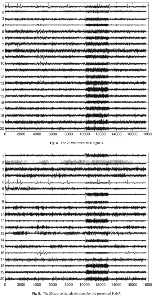
The MEG data set studied in this section consists of preprocessed signals originating from 122-channel whole-scalp MEG measurements from the brain [32,33]. The original signals are band-pass filtered between 0.5 and 45 Hz, and the data dimension is reduced from 122 to 20 using the principal component analysis (PCA) whitening approach to reduce noise and over-learning. The record lasts 2 min and includes 17730 samples and the 20 whitened signals are illustrated inFig. 4.

(6)

Fig. 2. Average performance indexes over 100 independent runs for 5 sources with square temporal autocorrelation.

Fig. 3. Average performance indexes over 100 independent runs for 5 sources with square temporal autocorrelation when the outliers are introduced.

Fig. 5shows the extracted 20 nonlinear autocorrelation source signals with the proposed FixNA approach (usingG

(

u

)

=

log

(

cosh

(

u

))

). It is known that some of extracted source signals have clear physical or physiological interpretation [32,33], i.e. the extracted source signals 5 and 16 correspond to eye movements, 7 and 8 are related to the muscular activities, the signal 2 corresponds to the heart beating, and 17 shows clearly the artifact originated from the digital watch.

5. Conclusions

We have proposed the FixNA algorithm for blind source separation based on the nonlinear autocorrelation of source signals and have analyzed its stability conditions. We show that the BSS problem can be solved by maximizing the nonlinear temporal autocorrelation of sources. When sources have square temporal autocorrelation, we demonstrated the efficient implementation of the method. Also, the proposed FixNA can extract the artifacts in brain MEG data analysis. Thus, the FixNA algorithm, which is based on the nonlinear measure of temporal autocorrelations of sources, provides a novel statistical property to perform BSS.

(7)

Fig. 4. The 20 whitened MEG signals.

(8)

Acknowledgments

The authors wish to gratefully thank all anonymous reviewers who provided insightful and helpful comments.

References

[1] S.I. Amari, A. Cichocki, H. Yang, A new learning algorithm for blind source separation, in: Advances in Neural Information Processing Systems, vol. 8, 1996, pp. 757–763.

[2] A.K. Barros, A. Cichocki, Extraction of specific signals with temporal structure, Neural Computation 13 (9) (2001) 1995–2003.

[3] A. Bell, T. Sejnowski, An information-maximization approach to blind separation and blind deconvolution, Neural Computation 7 (6) (1995) 1129–1159.

[4] A. Belouchrani, K.A. Meraim, J.-F. Cardoso, E. Moulines, A blind source separation technique based on second order statistics, IEEE Transactions on Signal Processing 45 (2) (1997) 434–444.

[5] J.-F. Cardoso, B.H. Laheld, Equivariant adaptive source separation, IEEE Transactions on Signal Processing 44 (12) (1996) 3017–3030. [6] A. Cichocki, S.-I. Amari, Adaptive Blind Signal and Image Processing: Learning Algorithms and Applications, Wiley, New York, 2002. [7] P. Comon, Independent component analysis—a new concept? Signal Processing 36 (1994) 287–314.

[8] A. Hyvärinen, Fast and robust fixed-point algorithms for independent component analysis, IEEE Transactions on Neural Networks 10 (3) (1999) 626–634.

[9] A. Hyvärinen, Complexity pursuit: Separating interesting components from time-series, Neural Computation 13 (4) (2001) 883–898.

[10] A. Hyvärinen, Blind source separation by nonstationarity of variance: A cumulant-based approach, IEEE Transactions on Neural Networks 12 (6) (2001) 1471–1474.

[11] A. Hyvärinen, J. Karhunen, E. Oja, Independent Component Analysis, Wiley, New York, 2001.

[12] C. Jutten, J. Herault, Blind separation of sources, part I: An adaptive algoritnm based on neuromimetic architecture, Signal Processing 24 (1991) 1–10. [13] T.-W. Lee, M. Girolami, T. Sejnowski, Independent component analysis using an extended infomax algorithm for mixed subgaussian and supergaussian

sources, Neural Computation 11 (2) (1999) 417–441.

[14] M.S. Lewicki, T.J. Sejnowski, Learning overcomplete representations, Neural Computation 12 (2) (2000) 337–365.

[15] Y.Q. Li, A. Cichocki, S.I. Amari, Analysis of sparse representation and blind source separation, Neural Computation 16 (6) (2004) 1193–1234. [16] W. Lu, J.C. Rajapakse, Eliminating indeterminacy in ICA, Neurocomputing 50 (2003) 271–290.

[17] D.G. Luenberger, Optimization by Vector Space Methods, John Wiley, New York, 1969.

[18] K. Matsuoka, M. Ohya, M. Kawamoto, A neural net for blind separation of nonstationary signals, Neural Networks 8 (3) (1995) 411–419.

[19] L. Molgedey, H.G. Schuster, Separation of a mixture of independent signals using time delayed correlations, Physical Review Letters 72 (23) (1994) 3634–3637.

[20] E. Oja, M.D. Plumbley, Blind separation of positive sources by globally convergent gradient search, Neural Computation 16 (9) (2004) 1811–1825. [21] D.-T. Pham, J.-F. Cardoso, Blind separation of instantaneous mixtures of non stationary sources, IEEE Transactions on Signal Processing 49 (9) (2001)

1837–1848.

[22] M.D. Plumbley, E. Oja, A “non-negative PCA” algorithm for independent component analysis, IEEE Transactions on Neural Networks 15 (1) (2004) 66–76.

[23] J.V. Stone, Blind source separation using temporal predictability, Neural Computation 13 (2001) 1559–1574.

[24] Z. Shi, H. Tang, Y. Tang, A new fixed-point algorithm for independent component analysis, Neurocomputing 56 (2004) 467–473.

[25] Z. Shi, H. Tang, Y. Tang, Blind source separation of more sources than mixtures using sparse mixture models, Pattern Recognition Letters 26 (16) (2005) 2491–2499.

[26] Z. Shi, H. Tang, Y. Tang, A fast fixed-point algorithm for complexity pursuit, Neurocomputing 64 (2005) 529–536. [27] Z. Shi, C. Zhang, Gaussian moments for noisy complexity pursuit, Neurocomputing 69 (7–9) (2006) 917–921. [28] Z. Shi, C. Zhang, Energy predictability to blind source separation, Electronics Letters 42 (17) (2006) 1006–1008.

[29] Z. Shi, C. Zhang, Semi-blind source extraction for fetal electrocardiogram extraction by combining non-Gaussianity and time-correlation, Neurocomputing 70 (2007) 1574–1581.

[30] Z. Shi, C. Zhang, Nonlinear innovation to blind source separation, Neurocomputing 71 (2007) 406–410.

[31] L. Tong, R.-W. Liu, V. Soon, Y.-F. Huang, Indeterminacy and identifiability of blind identification, IEEE Transactions on Circuits and Systems 38 (5) (1991) 499–509.

[32] R. Vigário, V. Jousmaäki, M. Hämäläinen, R. Hari, E. Oja, Independent component analysis for identification of artifacts in magnetoencephalographic recordings, Advances in Neural Information Processing Systems 10 (1998) 229–235.

[33] R. Vigário, J. Särelä, V. Jousmaäki, M. Hämäläinen, E. Oja, Independent component approach to the analysis of EEG and MEG recordings, IEEE Transactions on Biomedical Engineering 47 (5) (2000) 589–593.

[34] H. Zhang, C. Guo, Z. Shi, E. Feng, A new constrained fixed-point algorithm for ordering independent components, Journal of Computational and Applied Mathematics, in press (doi:10.1016/j.cam.2007.09.010).