Net present value analysis of the economic production quantity

(1)

IMA Journal of Management Mathematics(2013) Page 1 of 13 doi:10.1093/imaman/dpt002

Net present value analysis of the economic production quantity

Stephen M. Disney∗

Logistics Systems Dynamics Group, Cardiff Business School, Cardiff University, Cardiff CF10 3EU, UK

∗_{Corresponding author: [email protected]} Roger D. H. Warburton

Department of Administrative Sciences, Metropolitan College, Boston University, Boston, MA 02215, USA

[email protected] and

Qing Chang Zhong

Department of Automatic Control and Systems Engineering, University of Sheffield, Mappin Street, Sheffield S1 3JD, UK

[email protected]

[Received on 25 December 2011; accepted on 22 January 2013]

Using Laplace transforms we extend the economic production quantity (EPQ) model by analysing cash flows from a net present value (NPV) viewpoint. We obtain an exact expression for the present value of the cash flows in the EPQ problem. From this, we are able to derive the optimal batch size. We obtain insights into the monotonicity and convexity of the present value of each of the cash flows, and show that there is a unique minimum in the present value of the sum of the cash flows in the extended EPQ model. We also obtain exact point solutions at several values in the parameter space. We compare the exact solution to a Maclaurin series expansion and show that serious errors exist with the first-order approximation when the production rate is close to the demand rate. Finally, we consider an alternative formulation of the EPQ model when the opportunity cost of the inventory investment is made explicit. Keywords: economic production quantity; net present value; Lambert W function; Maclaurin series expansion.

1. Introduction

It is 100 years since the introduction of the economic order quantity (EOQ) formula by Ford Whitman Harris in 1913.Erlenkotter (1990) provides an excellent historical review of its early development. While some authors question the relevance of this approach in the current ‘lean’ environment (see, for example,Voss,2010), it is our experience that the EOQ philosophy is still important today, especially in process industries where expensive production capacity is required to produce several similar products. Indeed, both American (see, for example,Blackburn & Scudder,2009;Grubbström & Kingsman,2004) and European (see,Beullens & Janssens,2011;Disney & Warburton,2012) academic outlets are still regularly publishing papers on the subject. Furthermore, it is our experience that industry still finds this a valuable managerial tool.

c

at Cardiff University on February 25, 2013

http://imaman.oxfordjournals.org/

(2)

Shortly after Harris introduced the EOQ solution,Taft(1918) generalized the approach in what is now known as the economic production quantity (EPQ) problem. The main difference between the EPQ model and the EOQ model is that the EPQ model assumes that it takes time to produce the batch quantity, whereas the EOQ model assumes that the entire batch arrives instantaneously, all in one go.

There are many variations and extensions to both the EOQ and EPQ models in the literature. Many of these problems have exact explicit solutions, but most of the more complicated variations require heuristic approaches or exploit approximations. It appears that the first paper to consider the time value of money in an EOQ/EPQ inventory model isHadley(1964), where a numerical approach was taken. The contribution ofGrubbström(1980) makes the link between net present value (NPV) and the Laplace transform of the cash flows in the EPQ model. Here, an expression for the NPV of the cash flows in the EPQ model and its equivalent Annuity Stream is derived, but no attempt is made to identify the exact optimal batch quantity, rather a Maclaurin expansion is used to obtain an approximate solution.

Grubbström & Kingsman (2004) consider the NPV of an EOQ decision when it is known that there will be a future price increase. An interesting feature of that problem is that the batch size is dynamic in time, with large orders placed in the final moment before the price increase.

Recently,Warburton(2009) noticed that some EOQ problems that were thought not to have exact, explicit solutions can be solved by employing the Lambert W function. Disney & Warburton(2012) integrated the Laplace transform and the Lambert W function in an investigation of two different EOQ problems: an EOQ problem with perishable inventory and the NPV of an EOQ problem with yield loss. They are able to obtain exact, explicit solutions for the optimal batch size in both these problems, and it is this approach that we follow here to study the NPV of the cash flows in the EPQ problem.

In Section 2, we define the EPQ problem from an average cost perspective. Section 3 considers the EPQ problem from the NPV perspective and Section 4 undertakes a numerical investigation to demonstrate the validity and practical utility of the theoretical model. Here, we also compare the exact solution to an approximation based on the Maclaurin expansion. Section 5 provides some conclusions.

2. The economic production quantity

We briefly review the classical EPQ model and its derivation. Traditionally, the total annual cost (TC) is to be minimized. The cost is minimized by selecting a production batch size,Q∈ >0, whereQis the decision variable. The total cost is assumed to be made up of the cost of holding inventory (the cost of holding one unit of inventory for 1 year ish∈ 0); the cost of a production set-up isk∈ 0 (a change-over cost between one product and another) and the direct cost of production per unit is c∈ >0 (not including the holding or the set-up cost).

The external, and hence uncontrollable (at least not easily), variables are the demand rate,D∈ >0, and the production rate,P∈ D. It is usual to consider the EPQ operating on an annual basis, soD is the demand per year, and Pis the production per year that could be achieved if the product were manufactured continuously.PD, as otherwise the production would never be able to keep up with demand. WhenP>D, the product is manufactured intermittently, and it is this situation that is typically considered in an EPQ analysis. WhenP=Dwe produce continuously and never conduct a change-over. In the interval when we are not producing the product, we assume that the manufacturing equipment either lays idle or is used to manufacture another product. Access to production capacity is available instantly and at any time.

(3)

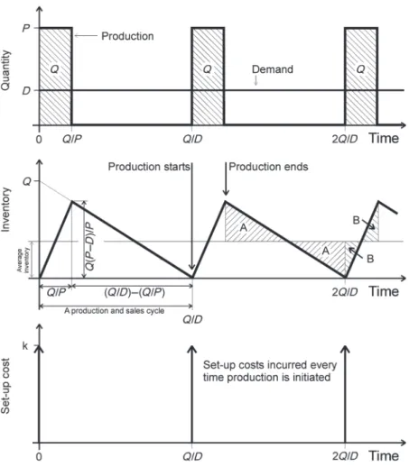
Fig. 1. The production, inventory, and set-up costs over time in the EPQ problem.

2.1 Time-based evolution of the costs

The direct production costs (cper unit) are incurred during the period when manufacturing product. As product is manufactured at a rate ofP, direct costs are incurred at a rate ofcP. AfterQitems have been made, the production is turned off (afterQ/Punits of time since production was started). During the period when production is running, asP>D, inventory has been building up (at a rate ofP−D). When production ceases, the inventory level is atQ(P−D)/Pand the inventory thereafter is depleted at a rate of−D. At the instant that inventory falls to zero (atQ/Dunits of time after the last set-up was conducted), we assume production starts again and inventory builds up. The average inventory being held at any point in the year isQ(P−D)/2P. Every time the production is started up, a production set-up cost ofkis incurred. There areD/Qsetups per year. Figure1sketches the time evolution of the three components of the EPQ costs.

(4)

Fig. 2. Block diagram of the cash flows in the EPQ problem.

From the above description, it is easy to obtain the following expression for the TC. TC=Dk

Q +

Qh(P−D)

2P +cD. (1)

Taking the derivative with respect toQyields the following equation: dTC dQ = Dk Q2 + h(P−D) 2P . (2)

Setting the derivative to zero and solving for the optimal batch quantity,Q∗, gives Q∗= 2PDk h(P−D)= 2Dk h P P−D. (3)

It is easy to verify thatQ∗ in (3) is indeed a minimum by taking the second derivative(d2_TC_/_d_Q2₌ 2Dk/Q3₎_{and noting that it is always positive when}_{_Q_,_D_,_k_{} ∈}_>_{0. We notice in (}₃_{) that the}_Q∗_{, given} by the EPQ model is always bigger than the EOQQ∗ as√P/(P−D) >1 whenP>D. Furthermore, increasing the production ratePresults in a smallerQ∗, and indeed, whenP→ ∞we regain the EOQ result. As in the EOQ case, reducing the set-up cost,k, results in smaller optimal order quantities. 3. Net present value analysis of the EPQ problem

Grubbström(1967) showed that if a Laplace transform is used to describe a cash flow over time and the Laplace operator,s, has been replaced by the continuous discount rater, then the Laplace transform, F(s), of the cash flow,f(t), yields the present value (PV) of the cash flow. This fundamental relationship is formalized as follows: PV= F(s)= _∞ 0 e−stf(t)dt s=r . (4)

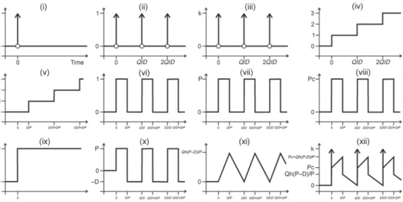
Using some rather basic control engineering knowledge (seeNise,1995;Buck & Hill,1971) we may develop a block diagram to describe the cash flows in the EPQ system, see Fig.2. From this we will later obtain the Laplace transform of the cash flows in the EPQ model. Figure3illustrates the time-based evolution of each of the signals in the EPQ problem showing how the cash flows are constructed.

(5)

Fig. 3. Time evolution of the signals that generate the cash flows in the EPQ problem.

Grubbström (1980) argued that the inventory holding costs are unnecessary in the EPQ case, as they have already been accounted for in the production cost cash flow. IndeedHarris (1913) defined inventory holding costs as an opportunity cost related to the production cost. We have elected to include them as we note that, besides the capital inventory cost, there may be other out-of-pocket expenses such as storage, spoilage, shrinkage and insurance to be accounted for. However, if these out-of-pocket costs can indeed be ignored as advocated byGrubbström(1980), this can easily be modelled by settingh=0. The block diagram in Fig.2may be manipulated to obtain the following Laplace transform transfer function that also describes the PV of the cash flows in the EPQ decision.

PVCosts=K(Q)+C(Q)+H(Q), (5) where K(Q)= k 1−e−Qs_/D; C(Q)= cP(1−e−Qs/P) s(1−e−Qs_/D₎ ; H(Q)= hP(1−e−Qs/P) s2₍₁₋_e−Qs_/D₎ − hD s2 . (6) Equation (5) can be reduced to

PVCosts=

e−Qs_/P₍_eQs_/P₍_Dh₊_eQs_/D₍_h₍_P₋_D₎₊_s₍_cP₊_ks₎₎₎₋_eQs_/D_P₍_h₊_cs₎₎

(eQs_/D₋₁_)s2 . (7)

We first study the PV of each of the costs individually. The PV of the set-up costs,K(Q), is shown in the first term in (5) and they are

• monotonically decreasing in Qas the first derivative, dK(Q)/dQ= −e−Qs/D_ks/D(₁₋_e−Qs/D₎2 0∀{s,k,Q,D}>0;

(6)

• strictly convex inQas d2_K₍_Q₎

dQ2 =

eQs_/D₍₁₊_eQs_/D₎_ks2

D2₍_eQs_/D₋₁₎3 >0 ∀{s,k,Q,D}>0; • infinite whenQ=0; and

• kwhenQ→ ∞.

The PV of the production costs,C(Q):

• are monotonically increasing inQas the first derivative, dC(Q)

dQ =ce

Qs(1/D−1/P)_(D(

eQs/D−1)+P(1−eQs/P))D(eQs/D−1)20 ∀{s,c,Q,D,P}>0, a relationship that is more obvious to determine from

C(Q)=cP s 1−e−Qs/P 1−e−Qs_/D ,

as both the numerator and denominator of the bracketed term are non-decreasing functions ofQ in the range(0, 1);

• are not concave inQas the second derivative d2_C(Q) dQ2 Q₌0 =cs(D(2D−3P)+P2) 6DP2

is positive whenDP2D. WhenP>2Dthe PV of the production costs appear to be concave inQ; • C(Q)=cD s and dC(Q) dQ Q=0 =c(P−D) 2P whenQ=0; • C(Q)=cP s and dC(Q) dQ Q_→∞ = d2C(Q) dQ2 Q_→∞ =0 whenQ→ ∞. The PV of the inventory costs,H(Q), (the third component of (5)):

• are monotonically increasing inQas the first derivative dH(Q)

dQ =

heQs(1/D−1/P)_(D(_eQs/D₋₁₎₊_P(₁₋_eQs/P₎₎

Ds(eQs/D−₁)2 0 ∀{s,h,Q,D,P}>0. Again this relationship is more obvious to determine from

H(Q)=hP s2 1−e−Qs/P 1−e−Qs/D −hD s2

as both numerator and denominator of the bracketed term are non-decreasing functions ofQin the range(0, 1);

(7)

• are not concave inQas the second derivative d2_H₍_Q₎ dQ2 Q=0 =h(D(2D−3P)+P2) 6DP2

is positive whenDP2D. WhenP>2Dthe PV inventory costs appear to be concave inQ;

• H(Q)=0 and dH(Q) dQ Q=0 =h(P−D) 2Ps whenQ=0; • H(Q)=h(P−D) s2 and dH(Q) dQ Q→∞ = d2H(Q) dQ2 Q→∞ =0 whenQ→ ∞.

As both the PV of the production and inventory costs are monotonically increasing functions ofQ, their sum is also a monotonically increasing function ofQ. The PV of the set-up costs are monotonically decreasing inQ. It then follows that the PV of the sum of all three costs in the EPQ model has a unique minimum inQ.

Taking the derivative of (5) with respect toQyields dPVCosts

dQ =

e(1/D−1/P)Qs₍₍_D₍_eQs/D₋₁₎₊_P₎₍_h₊_cs₎₋_eQs/P₍_hP₊_s₍_cP₊_ks₎₎₎

Ds(eQs_/D₋₁₎2 , (8)

from which the following characteristic equation can be obtained that describes the optimal batch size Q∗_NPV:

(D(eQ∗NPVs/D−₁)+P)(h+cs)−_eQ∗NPVs/P(hP+s(cP+ks))=_0. ₍₉₎ Equation (9) can be rearranged into the following formAeaQ∗_NPV₊_B_ebQ∗_NPV₊_C₌_{0 where}

a= s D; A=D(h+cs); b= s P; B=P(cs+h)+ks2; C=P(cs+h)−D(h+cs). (10)

In (9), while all the variables are real, there is no known general solution to this equation. However, we are able to obtain solutions at specific points in the parameter space. When the production rate,P, is less than (or equal to) the demand rateD, then it is best to produce continuously, forever (as the production rate cannot keep up with demand), so,

Q∗|PD= ∞ (11)

holds. This can also be verified by letting P→D in (5) and simplifying to yield PVCosts=k+ k/(eQs/D₋₁₎₊_(cD/s)_{, which is clearly minimized when}_Q_{→ ∞}_.

(8)

Although (9) has no general solution, point solutions can be obtained whenP/D= {1, 2, 3. . .}. For example, the solution atP=2Dis

Q∗_NPV|P₌2D= P s Log hP+cPs+ks2+4D(D−P)(h+cs)2₊_(hP₊_s(cP₊_ks))2 2D(h+cs) , (12)

and the solution atP=3Dis

Q∗_NPV|P=3D= P sLog ⎡ ⎢ ⎢ ⎢ ⎢ ⎣ 231/3_D₍_h₊_cs₎₍_hP₊_s₍_cP₊_ks₎₎₊√3 23 [9D3₍_h₊_cs₎3₋₉_D2_P₍_h₊_cs₎3₊√₃ D3₍_h₊_cs₎3₍₂₇_D₍_D₋_P₎2₍_h₊_cs₎3₋₄₍_hP₊_s₍_cP₊_ks₎₎3_)]2 3 √ 62_D₍_h₊_cs₎3 9D3₍_h₊_cs₎3₋₉_D2_P₍_h₊_cs₎3₊√₃_D3₍_h₊_cs₎3₍₂₇_D₍_D₋_P₎2₍_h₊_cs₎3₋₄₍_hP₊_s₍_cP₊_ks₎₎3₎ ⎤ ⎥ ⎥ ⎥ ⎥ ⎦. (13) This approach can be exploited further and solutions found atP=4Detc., but the equations become rather lengthy, so we will not present them. When the production rate,P, is infinite, the batch is delivered instantaneously, all at once. The solution in the limit whereP→ ∞is

Q∗_NPV|P_↑∞= − ks h+cs− D s 1+W₋1 −exp −1− ks 2 D(h+cs) , (14)

whereW₋1[x] is the LambertW function, evaluated on the alternative branch. We note that this is the solution for the EOQ problem given byWarburton(2009).Disney & Warburton(2012) provide some pedagogical insights on how to use the Lambert W function for EOQ problems in classroom settings. 4. Numerical investigations

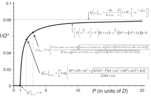
It is interesting to numerically investigate the impact ofPon the optimal batch sizeQ∗_NPV. Consider the industrially relevant case detailed inDisney & Warburton(2012) of annual demandD=18, discount rates=0.2, order placement costk=27, direct costc=10 and inventory holding costh=4.

This is illustrated in Fig.4, where we have plotted 1/Q∗_NPV for convenience. Here asP becomes much greater thanD,Q∗_NPVapproaches the EOQ solution asymptotically. Furthermore whenPis only just greater thanD,Q∗_NPVis rather large.

Figure5shows the PV of the costs whenQ=Q∗_NPV. We can see that in our numerical example the PV ranges from 917 to 1300 and is increasing inP. If the NPV EOQQ∗is used (14) instead ofQ∗_NPV then the percentage increase in the PV of the costs falls quite rapidly from 28.7% atP=Dto 9% when P=2D, 5.7% atP=3D, 3.3% atP=5D, 2% atP=8Dand less than 1% whenP>16D. So although the error is significant in practical situation whenPis close toD, (14) provides a useful near-optimal solution whenPD, when there is no appetite to calculateQ∗_NPV from (9). However, we note that (9) is quite easily determined with the help of a good scientific calculator or with the Microsoft Excel Solver function.

4.1 Approximations to the optimal batch size

The first-order Maclaurin expansion of (7) yields the following power series for the PV of the costs PVCosts≈ k 2+ D(k+cQ) sQ + kPs2+6D(h+cs)(PQ−D) 12sDP +O[Q] 2_. ₍₁₅₎

(9)

Fig. 4. The optimal order quantity in the NPV EPQ problem.

Fig. 5. Cost performance of the NPV EPQ model and the NPV EOQ solution.

Taking the derivative of (15) with respect toQand solving for the first-order conditions yieldsQ∗₂, an approximate value ofQ∗_NPV, the optimal batch quantity when the NPV of the cash flow is accounted for

Q∗₂= 2D

√

3kP

kPs2₋₆_D2_(h₊_cs)₊₆_DP(h₊_cs). (16) Figure6shows the percentage error between the Maclaurin expansion and the optimal batch quantity for minimizing the of the costs in the EPQ decision,Q∗_NPV. The numerical example chosen in this figure

(10)

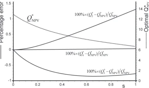
Fig. 6. Accuracy of the Maclaurin expansion for determining the optimal batch quantity.

isD=10,P=25,k=20,c=10,h=4. Here, we have plotted the errors for the first-,Q∗₂, second-,Q∗₃ and third-order,Q∗₄, Maclaurin expansions. The second- and third-order Maclaurin expansions for the PV of the costs are

PVCosts≈ k 2+ D(k+cQ) sQ + kPs2₊₆_D(h₊_cs)(PQ₋_D) 12sDP +Q2(h+cs)(D−P)(2D−P) 12DP2 +O[Q] 3 ₍₁₇₎ and PVCosts≈ k 2 + D(k+cQ) sQ + kPs2₊₆_D₍_h₊_cs₎₍_PQ₋_D₎ 12sDP +Q2(h+cs)(D−P)(2D−P) 12DP2 −(sQ3(30D2(D−P)2(h+cs)+kP3s2)) 720D3_P3 +O[Q] 4 ₍₁₈₎

but we have not re-arranged them forQ∗₃ andQ∗₄ as the results are very lengthy. These higher order expansions do indeed lead to more accurate approximations forQ∗_NPV, as shown in Fig.6.

The second-order error appears to be increasing in as the discount rate,s, increases for this numerical setting. The first- and second-order errors are around 1% for 0<s<0.8. The third order error is rather small. We also note that whenPis close toDthen the second- and third-order Maclaurin expansions

(11)

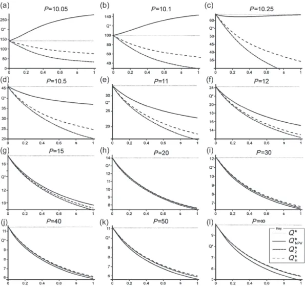
Fig. 7. The effect ofPonQ∗whenD=10,k=20,c=10 andh=4.

are numerically difficult to evaluate. As

Q∗₂|s_→0=Q∗NPV|s_→0=Q∗= 2PDk h(P−D), dQ∗₂ ds = 2D√3kP(3cD(D−P)−kPs) (kPs2+₆D(P−D)(h+cs))3/2 <0 ∀s, (19) andPD, thenQ∗₂<Q∗when s>0 andQ∗₂ is strictly decreasing ins. From this fact we might pro-pose that Q∗_NPV<Q∗ when s>0. However, this is erroneous reasoning as numerical investigations, which are illustrated in Fig.7, reveal that whenPis close toD,Q∗_NPVis actually an increasing function

(12)

ins, see plots (a) and (b). This demonstrates a fundamental structural difference between the behaviour of the first-order Maclaurin expansion and the true behaviour. Plot (c) shows thatQ∗_NPV is initially a decreasing function ins, but then becomes an increasing function issnears=0.298 (it then becomes a decreasing function again nears=1.224, but this is not shown). Furthermore, we can see from Fig.7

that sometimes the Maclaurin series expansion under-estimatesQ∗_NPV[see plots (a) to (i)], and at other times it is an over-estimate [see plots (j) to (k)]. In Fig. 7we have also highlighted the value of the classic EPQ, Q∗, as well at the case when the Production rate,P, becomes infinite (the EOQ) case, plot (l).

Grubbström (1980) argues for an alternative formulation of the EPQ model. In our situation it amounts to replacing h, the unit inventory holding cost with(h+cs), where h is the out-of-pocket inventory costs andcsis the opportunity cost of the inventory investment. This leads to the following annual total cost function:

TCH=cD+

Dk

Q +

(P−D)Q(h+cs)

2P (20)

which has the following, first- and second-order derivatives w.r.t.Q dTCH dQ = (P−D)(h₊_cs) 2P − Dk Q2, d2_TC H dQ2 = 2Dk Q3 (21)

from which we may obtain the following expression forQ∗H, an optimal production quantity when the

opportunity costs from the inventory investment have been explicitly linked to the discount rates,

Q∗H=

2kDP

(h₊_cs)(P₋_D). (22)

We have also plottedQ∗Hin Fig.7. We can see that although it has the same structural deficiencies

as the first-order Maclaurin expansion approximation, it is more accurate whenPis relatively small [in plots (a) to (h)]. Furthermore, it is only marginally less accurate than the first-order Maclaurin expansion approximation whenPis large [see plots (i) to (l)]. We propose, therefore, that the simple expression (22) is at least as useful as the approximation given first-order Maclarurin series expansion. Indeed it may be very useful when thePis reasonably larger thanQ.

5. Concluding remarks

We have enhanced the EPQ model by including the PV of the cash flows. To capture the PVs, we exploited the Laplace transform. We focused on identifying the influence on the optimal batch size, Q∗_NPV, of the PV of the costs. We have obtained important managerial insights into the monotonicity and convexity of each of the costs in the EPQ model, and have shown that there is a unique batch quantity that minimizes the PV of the cash flows.

We were able to obtain an exact expression for the NPV of the EPQ problem in terms of a charac-teristic equation for the optimal batch sizeQ∗_NPV. We were also able to obtain exact point solutions in the parameter space, and showed that the Lambert W function plays an important role in the case where the production ratePis large compared with the demand rateD. We were unable to obtain a complete explicit solution to the equation forQ∗_NPV. However, numerical solutions to the characteristic equation given in (9) can easily be obtained using either a scientific calculator or the Excel Solver.

(13)

We have compared our results to a Maclaurin series expansion of the NPV of the cash flows and found that the first-order series expansion results in structurally erroneous insights asQ∗_NPVcan become greater than theQ∗. However, this appears (only) to happen only whenPis very close to (but still greater than)D. We have also investigated an alternative formulation of the EPQ model when the opportunity cost of the inventory investment is linked to the discount rates. Although this EPQ formulation suffers from the same limitation of the first-order Maclaurin approximation, it appears to be more accurate whenPis not too large. WhenPis sufficiently greater (and numerical investigation seem to suggest that sufficiently greater is not that much greater) thanD, thenQ∗_NPV<Q∗. This may help explain why the EPQ/EOQ approach is often ignored by the Lean Production community who frequently advocate that the production batch quantity,Q, should be a small as practically possible.

Acknowledgements

We thank the referees and editors for some useful suggestions that have significantly improved this paper.

References

Beullens, P. & Janssens, G. K.(2011) Holding costs under push or pull conditions—the impact of the anchor

point.Eur. J. Operat. Res.,215, 115–125.

Blackburn, J. & Scudder, G.(2009) Supply chain strategies for perishable products: the case of fresh produce. Prod. & Oper. Manag.,18, 127–137.

Buck, J. R. & Hill, T. W.(1971) Laplace transforms for the economic analysis of deterministic problems in

engineering.Eng. Econom., 16, 247–263.

Disney, S. M. & Warburton, R. D. H.(2012) On the Lambert W function: economic order quantity applications

and pedagogical considerations.Int. J. Prod. Econ.,40, 756–764.

Erlenkotter, D.(1990) Ford Whitman Harris and the economic order quantity model.Oper. Res.,38, 937–946.

Grubbström, R. W.(1967) On the application of the Laplace transform to certain economic problems.Manag.

Sci.,13, 558–567.

Grubbström, R. W.(1980) A principle for determining the correct capital costs of work-in-progress and inventory. Int. J. Prod. Res.,18, 259–271.

Grubbström, R. W. & Kingsman, B. G.(2004) Ordering and inventory policies for step changes in the unit item

cost: a discounted cash flow approach.Manag. Sci.,50, 253–267.

Hadley, G.(1964) A comparison of order quantities computed using the average annual cost and the discounted

cost.Manag. Sci.,10, 472–476.

Harris, F. W.(1913) How many parts to make at once.Factory Mag. Manag.10, 135–136, 152. Reprinted inOper.

Res., 1990,38, 947–950.

Nise, N. S.(1995)Control Systems Engineering. Redwood, CA: Benjamin Cummings.

Taft, E. W.(1918) The most economical production lot.Iron Age,101, 1410–1412.

Voss, C. (2010) Thoughts on the state of OM. http://om.aomonline.org/dyn/news/Editorial_Voss.pdf. Verified 6 November 2011.

Warburton, R. D. H.(2009) EOQ extensions exploiting the Lambert W function.Eur. J. Ind. Eng.,3, 45–69.