The robustness of seismic attenuation measurements using
fixed- and variable-window time-frequency transforms
Carl Reine
1, Mirko van der Baan
1, and Roger Clark
1ABSTRACT
Frequency-based methods for measuring seismic attenuation are used commonly in exploration geophysics. To measure the spectrum of a nonstationary seismic signal, different methods are available, including transforms with time windows that are either fixed or systematically varying with the frequency being ana-lyzed. We compare four time-frequency transforms and show that the choice of a fixed- or variable-window transform affects the robustness and accuracy of the resulting attenuation measure-ments. For fixed-window transforms, we use the short-time Fou-rier transform and Gabor transform. The S-transform and contin-uous wavelet transform are analyzed as the variable-length trans-forms. First we conduct a synthetic transmission experiment, and compare the frequency-dependent scattering attenuation to the theoretically predicted values. From this procedure, we find that variable-window transforms reduce the uncertainty and bias
of the resulting attenuation estimate, specifically at the upper and lower ends of the signal bandwidth. Our second experiment mea-sures attenuation from a zero-offset reflection synthetic using a linear regression of spectral ratios. Estimates for constant-Q at-tenuation obtained with the variable-window transforms depend less on the choice of regression bandwidth, resulting in a more precise attenuation estimate. These results are repeated in our analysis of surface seismic data, whereby we also find that the at-tenuation measurements made by variable-window transforms have a stronger match to their expected trend with offset. We con-clude that time-frequency transforms with a systematically vary-ing time window, such as the S-transform and continuous wave-let transform, allow for more robust estimates of seismic attenua-tion. Peaks and notches in the measured spectrum are reduced be-cause the analyzed primary signal is better isolated from the coda, and because of high-frequency spectral smoothing implicit in the use of short-analysis windows.
INTRODUCTION
Seismic attenuation can be caused by intrinsic effects such as ane-lastic losses resulting from fluid movement共Dvorkin and Nur, 1993兲
and friction between grains or crack faces共Johnston et al., 1979兲. Similarly, losses can occur by processes that mimic intrinsic effects such as multiple scattering. Typically, the overall effect on the seis-mic signal is that higher frequencies are suppressed more rapidly than lower frequencies as the signal propagates over greater distanc-es or through more attenuating media. This rdistanc-esults in a loss of signal resolution.
Conversely, the additional information that attenuation imparts to the signal can be a useful tool for reservoir characterization. For ex-ample, attenuation is sensitive to changes in gas saturation in partial-ly saturated media共Winkler and Nur, 1982兲, and in fractured media,
the magnitude of attenuation change with azimuth has been shown to be a useful indicator of fracture direction共Clark et al., 2001; Mault-zsch et al., 2007兲. Finally, once attenuation is measured, it is possible to mitigate the resolution loss by applying processes such as inverse-Qfiltering共Wang, 2002兲to aid with structural interpreta-tions共Kaderali et al., 2007兲, amplitude-variation-with-offset共AVO兲 analysis共Luh, 1993兲. Attenuation is therefore a desirable parameter to estimate; however, effects on the seismic spectrum from interfer-ence of different seismic arrivals often make its accurate determina-tion elusive.
Among the many methods available for measuring seismic atten-uation, frequency-based methods are common in exploration geo-physics because of their reliability and ease of use共Tonn, 1991兲. Spectral estimates are required for these methods, which often are obtained using the short-time Fourier transform共STFT兲 共Dasgupta
Manuscript received by the Editor 20 March 2008; revised manuscript received 18 July 2008; published online 11 March 2009.
1University of Leeds, School of Earth and Environment, Earth Sciences, Leeds, U. K. E-mail: [email protected]; [email protected];
© 2009 Society of Exploration Geophysicists. All rights reserved.
and Clark, 1998;Hauge, 1981兲. Time-frequency transforms, such as the continuous wavelet transform共Chakraborty and Okaya, 1995;
Rioul and Vetterli, 1991兲and S-transform共Stockwell et al., 1996兲, are available also, and they are becoming more popular. The contin-uous wavelet transform has found success in spectral decomposition 共Sinha et al., 2005兲, and one of its benefits is its well-localized time extent, particularly at high frequencies.
A few investigations have compared different time-frequency transforms for specific applications. In the context of temporal reso-lution,Castagna and Sun共2006兲compare the performance of the STFT and wavelet transform with other spectral estimates. They ac-complish this by creating synthetic data using interfering wavelets of different frequencies, and they conclude that a variant of matching pursuit decomposition共Mallat and Zhang, 1993兲has the best tempo-ral resolution for their experiment. In the context of attenuation,Tai et al.共2006兲compare the STFT and wavelet transform for their abili-ties to produce attenuation estimates in the presence of Gaussian ran-dom noise. Their work uses the spectral ratio method applied to a source wavelet and an isolated and attenuated version. Other works show that non-Fourier transforms can be used for attenuation esti-mates共e.g.,Li et al., 2006兲, yet a formal comparison of transform types still is required in this context, and the aim of this paper is to provide this comparison.
The use of simple synthetics does not establish conclusively the superiority of one transform over another for attenuation estimates. Part of the issue with calculating a spectrum is that the seismic re-sponse is more complicated than a sparse convolutional model. The spectrum of recorded data is influenced by scattering losses and in-terference from short-path multiples共O’Doherty and Anstey, 1971;
Shapiro and Zien, 1993兲. By obtaining estimates of the spectrum that are less affected by this interference, more confident and stable at-tenuation estimates can be made.
To address the complications of measuring a seismic spectrum, an investigation is required that looks at the behavior of different trans-form types in the presence of multiple scattering from numerous re-flection interfaces. Here, we demonstrate that there are significant differences between the spectral estimates from two broad catego-ries of time-frequency transforms: those having time windows that are fixed, and those with windows that are systematically varying with the frequency being analyzed. In the category of fixed-time-window transforms, we consider the STFT with both Hamming and Gaussian window functions, the latter referred to as a Gabor trans-form共Carmona et al., 1998兲. For variable-time-window transforms, we use the S-transform, and the continuous wavelet transform with a Morlet wavelet共Daubechies, 1992兲.
A third class of transform, which we do not consider, deals with parametric methods including Burg autoregressive estimates and matching pursuit decomposition. These methods allow for signal de-composition with spectral elements whose size is flexible共Wang, 2007兲. Although this property is useful for compactly describing sig-nals or identifying major signal components, it makes a direct com-parison with convolutional methods difficult. Whereas the basis functions for the transforms that we consider remain constant, the el-ements of parametric methods change depending on the signal, and it is not possible to apply conclusions from testing these methods to the general case.
We introduce first the algebraic description of seismic wave atten-uation, and then give an overview of the time-frequency transforms
that we use. To test which transforms produce the most robust and least biased attenuation estimates, we conduct two synthetic experi-ments and an analysis of real-surface seismic data. First we compare estimated and theoretical attenuation profiles resulting from multi-ple scattering. For this purpose, we model a transmission vertical seismic profile共VSP兲and use wave localization theory共Shapiro and Zien, 1993兲to calculate the expected attenuation.
Next we estimate constant-Qeffective attenuation from a zero-offset reflection synthetic, and investigate the distribution of esti-mates for different bandwidths used in the linear regression of a nat-ural log spectral ratio versus frequency. We repeat this analysis on a common-midpoint共CMP兲supergather, and go on to investigate how well the measurements agree with expected behavior. Finally, we discuss reasons for the different performances, and the adequacy of each transform type for robust attenuation measurements.
THEORY Attenuation
The amplitude spectrum of a wave in a homogeneous attenuating medium is given by
S共f兲⳱S0共f兲eⳮ␣z, 共1兲 whereSis the amplitude of frequencyfafter propagating distancez, S0is the initial spectral amplitude, and␣is the attenuation coeffi-cient共Aki and Richards, 2002兲. By rearranging equation1, attenua-tion might be determined from the spectral estimates of an initialS0 and propagated eventS:
ln
冉
S共f兲S0共f兲
冊
⳱ ⳮ␣z. 共2兲Although there are many definitions relating␣and the seismic qual-ity factorQ共Toverud and Ursin, 2005兲, we use the definition given byAki and Richards共2002兲:
␣
⳱
fQV, 共3兲
whereVis the phase velocity of the wave in the medium.
Specifically for the case of a frequency-independentQ, by ex-pressing a combination of equations2and3in terms of traveltimet,
ln
冉
S共f兲S0共f兲
冊
⳱ ⳮ
tQf, 共4兲
a linear regression with frequency might be used to find the effective 1/Qefor the medium. The effective value, however, is not controlled just by intrinsic effects such as fluid flow, but is affected also by ap-parent attenuation effects such as multiple scattering. The effective 1/Qe is related to intrinsic 共1/Qi兲 and apparent 共1/Qsc兲 effects through the following relationship共Spencer et al., 1982兲:
1 Qe ⳱ 1 Qi Ⳮ 1 Qsc . 共5兲 Time-frequency transforms
A variety of methods are available to determine the spectra used in the measurement of 1/Q. For nonstationary data, time-frequency
transforms are useful, as they produce a spectral estimate centered at each time element of the data. In this respect, a 1D data trace is mapped into a 2D spectrogram, which has dimensions of time and frequency.
Perhaps the most recognized time-frequency transform is the STFT, in which the data tracesis gated by a sliding window function w, and the Fourier transform共Bracewell, 1978兲is applied to the re-sult:
SF共
,f兲⳱冕
ⳮ⬁ ⬁
w共tⳮ
兲s共t兲eⳮi2ftdt, 共6兲where is the time lag to the center of the window function. This definition allows for an arbitrary window function; however, by us-ing a Gaussian window function,
w共t兲⳱eⳮt2/22, 共7兲 whereis the distribution width, equation6takes on the definition of a Gabor transform共Carmona et al., 1998兲. This is because equa-tion6becomes a convolution of the signal with a modulated Gauss-ian function, which is the impulse response of a Gabor filter共Rioul and Vetterli, 1991兲.
For our STFT analysis, we use a Hamming function 共Harris, 1978兲, and for the Gabor transform, we use a fractional distribution width of⳱0.33. The time length of the windows is set at 101 ms for the following analysis. This is suitable for measuring frequencies above 10 Hz, which have a period smaller than the window size. For data with lower frequency content, a larger window must be used.
The window functions chosen for the STFT and Gabor transform have a fixed time length for each frequency that is analyzed. Con-versely, the S-transform共Stockwell et al., 1996兲analyzes shorter data segments as the frequencies increase. This is accomplished by using the Gaussian window function共equation7兲, and substituting a frequency-dependent expression for the distribution width:
⳱ 1兩f兩. 共8兲
Thus, by normalizing the window amplitude, the S-transform takes the form SS共
,f兲⳱冑
兩f兩 2
冕
ⳮ⬁ ⬁ s共t兲eⳮ共tⳮ兲2f2/2eⳮi2ftdt. 共9兲Whereas the above transforms use theeⳮi2ftbasis function, the
continuous wavelet transform uses scaled versions of a “mother wavelet”⌿as its basis共Daubechies, 1992兲. This results in a trans-form of the trans-form
SW共
,a兲⳱冑
1 a冕
ⳮ⬁ ⬁ s共t兲⌿
*冉
tⳮ
a冊
dt, 共10兲whereais the scale of the wavelet共Chakraborty and Okaya, 1995;
Rioul and Vetterli, 1991兲. Although no explicit window function is used, the basis function itself has a restricted time extent, and there-fore the time windowing is implicit in the choice of wavelet. Many mother wavelets exist, and as commonly done in seismic applica-tions, we use a modulated Gaussian, or Morlet, wavelet. This is de-fined byDaubechies共1992兲as
⌿
共t兲⳱
ⳮ1/4eⳮt2/2共eⳮi0tⳮeⳮ0 2/2兲, 共11兲 with the constant0defined by
0⳱
冑
2ln共2兲. 共12兲
After creating a high-frequency mother wavelet, the scaleais in-creased from its initial value. Thus, a time-scale decomposition is obtained, where increasing scaleacorresponds to decreasing fre-quency f. For comparison with other time-frequency transforms, each scale must be mapped to the frequency that corresponds to the center frequency of the scaled wavelet. This is done by calculating the expression for the Nyquist frequencyfNin the oscillatory term in equation11, and relating it to the initial frequency of the mother wavelet for discrete time withnpoints:
eⳮin⳱eⳮi0n. 共13兲 Therefore, the initial frequency of the mother wavelet is
f0⳱
0
fN, 共14兲 orf0⳱
02
⌬T, 共15兲where⌬Tis the sample rate of the data. The frequenciesfof subse-quent scalesathen are found as a function of the initial frequencyf0 by
f⳱1
af0. 共16兲
TRANSMISSION AND FREQUENCY-DEPENDENT ATTENUATION
Objective
The first test is a controlled experiment in which we compare esti-mated frequency-dependent attenuation with theoretically predicted profiles for a synthetic VSP. The purpose is to show that the type of transform used determines the precision and accuracy of the attenua-tion estimate. For this to be a meaningful test, two requirements must be met:共1兲a geophysical model with known attenuation must be cre-ated, and共2兲the seismic response of that model must be calculated to include all of the expected multiple reflections and interference. Al-though it is easy enough to design a finely layered model with known intrinsic attenuation, this does not account for the apparent attenua-tion caused by stratigraphic effects共O’Doherty and Anstey, 1971;
Schoenberger and Levin, 1974,1978;Spencer et al., 1977兲. Con-versely, a model with coarse layers might be created to isolate the in-trinsic attenuation; however, this does not accurately represent real-istic subsurface conditions.
Wave localization theory
To meet these conditions, we use wave localization theory, which describes the frequency-dependent attenuation of a transmitted wave caused by multiple scattering in a randomly layered medium 共Shapiro and Zien, 1993兲. By generating an appropriate medium, we compare the estimated attenuation to the theoretical attenuation at each frequency, thereby evaluating the quality of the spectral esti-mate. Because wave localization theory involves a statistical de-scription of the medium, it is possible then to create multiple model realizations and produce a statistical analysis of the attenuation esti-mates in terms of estimation variance and systematic error.
The random incompressibility fluctuations for a piecewise contin-uous medium display an exponential autocorrelation function,
共
兲⳱
2eⳮ兩兩/ac, 共17兲 whereis the autocorrelation function in terms of depth lag,is the relative standard deviation of the incompressibility fluctuations, andacis their characteristic scale length共van der Baan, 2001兲. For this type of medium, wave localization theory can be used to show that the theoretical apparent attenuation coefficient␣is given by␣
⳱
2
2a cf216ac2
2f2ⳭV2, 共18兲wherefis frequency andVis the average velocity共Shapiro and Zien, 1993;van der Baan, 2001兲.
This function shows how the energy of the primary arrival is scat-tered into a time-delayed sequence of arrivals referred to as the coda. Low frequencies, having larger wavelengths, see the random layer-ing as an effective medium, and the amount of scatterlayer-ing is negligi-ble. This results in apparent attenuation decreasing to zero in the low-frequency limit. The maximum scattering of energy occurs for frequencies with wavelengths that approach the typical scaleacof the medium. Finally, as frequencies increase, the attenuation coeffi-cient␣decreases and converges to a constant value because the me
dium is piecewise continuous and smaller wavelengths are resolved for each layer共van der Baan, 2001兲.
Test setup
Using the procedure outlined byvan der Baan et al.共2007兲, we an-alyze the sonic log of a well that penetrates a shallow sequence of al-ternating sands and shales. Assuming incompressibility fluctuations that observe an exponential autocorrelation function, and using a constant density, we then determine the parameters that describe the data. This is done by removing a polynomial trend from the velocity data, from which the zero-order term is used to give the mean veloci-ty. Next the autocorrelation function is calculated. The zero-lag val-ue of the autocorrelation, by equation17, gives the value of2. Sim-ilarly, the characteristic scale is the depth lag where
共ac兲⳱
2eⳮ1. 共19兲 We then use these parameters to create a reasonable set of model properties for our medium, as well as three variants of this model 共Table1兲. Following the method described byvan der Baan共2001兲, we generate 20 realizations of a random medium for each model, and from these produce VSP synthetics.We consider the vertical transmission of a seismic wave through 500 m of the random medium, with an overlying 11-m homoge-neous layer. An explosive source is placed at 10-m depth, and a re-ceiver is placed at 510 m. The modeling is done using a reflectivity method, as implemented byDietrich共1988兲, and to eliminate sur-face reflections, no free sursur-face is used in the computation of syn-thetic waveforms. The source used is a 70-Hz, 90° Ricker wavelet, and the intrinsic attenuation of the medium is made negligible by set-ting 1/Qi⳱10ⳮ6.
The signal spectrumS共f兲is extracted from the maximum ampli-tude coefficients for each frequency in the spectrogram. This allows for dispersion, because not all frequencies must have the same maxi-mum-amplitude arrival time. The reference-signal spectrumS0共f兲is obtained from an identical synthetic setup using a homogeneous me-dium, which eliminates potential problems resulting from geometric spreading and numerical dispersion共van der Baan, 2001兲. Finally, the estimated attenuation profiles are determined using equation2, and the 1/Qscis inspected using theAki and Richards共2002兲 defini-tion共equation3兲. The theoretical frequency-dependent 1/Qsccaused by scattering is obtained using equations3and18.
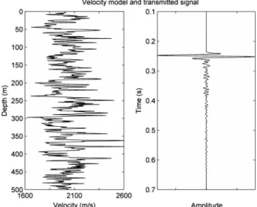
Results
Intermediate results are shown for only the first model from Table1, as the remaining models show similar effects. A single realization of the velocity model and the signal transmitted through it are displayed in Figure1. Here the time-domain effects of the multiple scattering are seen, where the direct arrival at 0.25 s is followed by coda en-ergy from the multiples. In Figure2, the spectro-gram of the transmitted signal is shown using the four transforms outlined above. The major differ-ence between the fixed-window transforms共 Fig-ure2aandb兲and the variable-window transforms 共Figure2candd兲is in the shape of the primary ar-rival in time-frequency space. This shape is
relat-Table 1. Measured and modeled parameters for a medium with random velocityvPfluctuations that exhibit an exponential autocorrelation. By
assuming a constant density, the relative standard deviation of the velocity
vis half of the relative standard deviation of incompressibility. Note that
although the scattering properties of models 2 and 3 are different, the apparent attenuation defined by equation18is the same for both.
Well-log analysis
Blocked
well log Model 1 Model 2 Model 3 Model 4
MeanVP共m/s兲 2037 2067 2000 2000 4000 2000
Mean共kg/m3兲 2104 2129 2100 2100 2100 2100
Relative共%兲 12.28 14.26 15 15 15 15
RelativeV共%兲 6.14 7.13 7.5 7.5 7.5 7.5
ed directly to the transform window size, and for the variable-win-dow transforms, the distinct wedge is evident, narrowing in time to-ward higher frequencies.
What is apparent also from Figure2is that the coda energy is not just separated from the direct arrival in time, but in frequency as
well. This is indicated by the lower amplitude energy centered be-tween 50 and 150 Hz, which follows the primary arrival at 0.26 s. More significant is that in the variable-window transforms, the coda energy above 100 Hz shows less interference with the primary ener-gy.
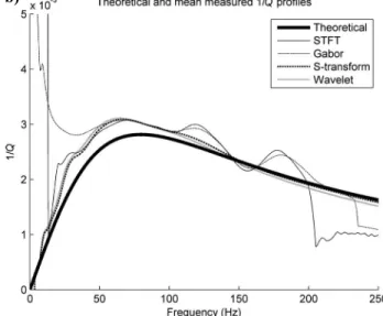
After extracting the maximum amplitude spectra from each trans-form, the respective 1/Qscfunctions are calculated for each realiza-tion, examples of which are shown in Figure3a. The frequency-de-pendent curves fluctuate significantly about the theoretical predic-tions as a result of the finite number of layers in the model, and the in-terference of the coda that results from multiple scattering. To ac-count for the finite layers, and to look at systematic deviations, we must take a look at the mean of the 1/Qscestimates from all realiza-tions.
The mean of the estimated attenuation from each transform is shown in Figure3b. The statistical fluctuations are reduced, and the main effects, which are visible, are fluctuations caused by coda inter-ference. Below 10 Hz and above 200 Hz, large variations result be-cause the measurements fall outside the significant bandwidth of the data. The deviations from the theoretical curves are similar for all of the transforms, with an improvement from the variable-window transforms for frequencies above 110 Hz and below 30 Hz.
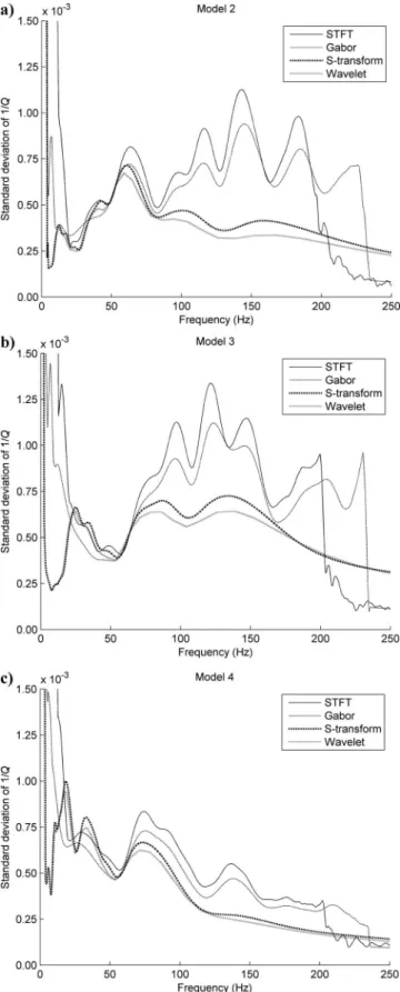
More significantly, the uncertainty in the measurement of a single realization is shown by the standard deviation of the distribution of estimates, shown in Figure3c. The standard deviation of the attenua-tion estimates is smaller for the variable-window transforms, with an exception of the frequencies between 30 and 55 Hz, where the re-sults show no major differences. In this frequency range, the window lengths for all of the transforms are similar. The most significant im-provements in the standard deviation are above 100 Hz. This suggests that individual amplitude spectra produced by the variable-window trans-forms are more precise, having a narrower statis-tical distribution. The analysis is repeated for models 2–4 from Table 1. Figure 4shows the standard deviations for the 1/Qscestimates for these models, and again, the results show that the variable-window transforms have a lower vari-ability than the fixed-window transforms, specifi-cally at higher frequencies.
Reducing the size of the time window in the STFT and Gabor transform obtains similar high-frequency results to the variable-window trans-forms. The detriment of reducing the time win-dow, however, is seen in Figure5, which shows one realization of the 1/Qscestimate from the STFT with different-length time windows. Al-though the fluctuations at high frequencies are re-duced, the minimum frequency for which 1/Q can be measured properly also increases. This is seen by the short-window curves, which have large deviations at the low end of the spectrum.
REFLECTION AND CONSTANTQ
ATTENUATION Objective
For the second experiment, we measure the ef-fective attenuation from a synthetic zero-offset Figure 1. A single realization of randomly fluctuating velocities
de-fined by the parameters of model 1共Table1兲, and the seismic signal transmitted through it. The coda follows the primary arrival after 0.26 s. Relative amplitudes are shown.
a)
c)
b)
d)
Figure 2. Time-frequency plots of the signal shown in Figure1. The highest amplitudes 共red colors兲are for the primary arrival, whose shape in the time-frequency domain is de-termined by the transform window functions. The interference effects between the pri-mary arrival and coda can be seen as “holes” in the spectrum.共a兲STFT,共b兲Gabor trans-form,共c兲S-transform, and共d兲 wavelet transform. The frequency axis of the wavelet transform has been rescaled to a linear frequency display.
surface seismic geometry. Because there is no simple analog to wave localization theory for reflection data, we use a different test to dem-onstrate the effects shown in the transmission experiment. We create a 1D model, which experiences a uniform constant-Qintrinsic atten-uation in addition to scattering losses.
Although frequency-dependent multiple scattering is present in all data, it is common to assume a frequency-independent effective 1/Qewithin the seismic bandwidth共Sams et al., 1997兲. This is a worthwhile first approximation as long as the frequency-indepen-dent intrinsic attenuation is large compared with the apparent scat-tering attenuation. The assumption also implies that an effective 1/Qeestimate from a linear regression of the natural log spectral ra-tio should be the same regardless of the bandwidth chosen. In fact, spectral fluctuations, which result in part from multiple scattering, cause the linear regression to be highly dependent on the choice of
bandwidth. This is true also for regressions that allow for a nonlinear relationship between the natural log spectral ratio and frequency 共Reid et al., 2001兲. In the second experiment, we test the ability of the time-frequency transforms to produce 1/Qeestimates that are robust with respect to the bandwidth used in the regression.
Test setup
We create first a 1D medium from the blocked velocity and densi-ty logs of the well data used in the transmission test. We impose a uniform intrinsic attenuation with 1/Qi⳱0.020, and produce zero-offset reflection seismic data with a 70-Hz, 90° Ricker source wave-let共Figure6兲. In Figure6, two reflectors are indicated that corre-spond to large velocity and density changes in the model. We extract the spectra from these two times and calculate the effective attenua-tion from a linear regression of their natural log spectral ratios, using
a)
c)
b)
Figure 3. The theoretical and estimated 1/Qscfor共a兲a single realization of the transmitted primary signal through the randomly fluctuating ve-locity model, and共b兲the mean of 20 realizations. The mean curve reduces statistical fluctuations for better analysis of the systematic deviations. The estimated frequency-dependent 1/Qscfluctuates about the theoretical curve resulting from effects of spectral interference with the coda en-ergy. The values are similar for all transforms, with a slight improvement from the variable-window transforms below 30 Hz and above 110 Hz. 共c兲Standard deviation of the 20 realizations of estimated 1/Qscshowing the frequency-dependent variability of the estimates. The variable-win-dow transforms show improvement below 25 Hz and above 90 Hz, indicating a more precise estimate.
equation2. Because initial and final spectra,S0共f兲andS共f兲, are sub-ject to scattering and interference, spectral notching exists in both, contrary to the transmission test in which only the final spectrum S共f兲was affected. We repeat the regression for different bandwidths, varying the lower frequency from 0 through 110 Hz, and the upper frequency between 90 and 250 Hz.
Although not strictly accurate, we use equations3and18to pro-vide a rough estimate of the scattering attenuation for the medium.
Figure 4.共a-c兲Standard deviations of estimated 1/Qscfor models 2-4, respectively. The improvement in the standard deviation for the variable-window transforms agrees with the data shown in Figure
3c.
Figure 5. Theoretical and estimated 1/Qscfor the single realization of the fluctuating velocity model shown in Figure1using different win-dow lengths of the STFT. Whereas the smaller winwin-dows reduce fluc-tuations at higher frequencies, the low frequencies are not measured properly.
Figure 6. From left to right, the blocked P-wave velocity and density logs, and the resulting zero-offset reflection synthetic共normal polar-ity with black peaks兲. The dashed lines at 164 and 310 m共159 ms and 309 ms兲indicate two major impedance changes whose reflec-tions are used in the 1/Qanalysis. The logs have been blocked with an average block size of 2 m.
Using the parameters calculated for the blocked well log in Table1, the maximum 1/Qscfor the medium occurs at 82 Hz and has a value of 1/Qsc ⳱0.003. Although not exact, this estimation shows that the apparent attenuation is an order of magnitude smaller than the imposed intrinsic at-tenuation for this model, consistent with observa-tions made bySams et al.共1997兲. The effective 1/Qefor the medium therefore should be approxi-mately 0.023共equation5兲.
Results
For each discrete bandwidth choice, a 1/Qe value is calculated and plotted in Figure7. In this plot, large areas of the same color indicate that the 1/Qeestimate is stable with the choice of band-width. Ideally, this stable value should corre-spond to the effective attenuation, a combination of the input intrinsic attenuation and apparent at-tenuation from multiple scattering. Areas at the extreme ends of the color scale indicate that the regression result is dominated by peaks and notches in the natural log spectral ratio.
Figure7aandb, for the fixed-window trans-forms, are similar in appearance. The most stable region that corresponds to the approximate 1/Qe is found roughly in the center of the plot, between 15 and 65 Hz on the vertical axis and 125 Hz through 200 Hz on the horizontal axis. The plots corresponding to the variable-window trans-forms, Figure7candd, extend this stable area back to nearly 0 Hz on the vertical axis, and out through 250 Hz on the horizontal axis. In prac-tice, the extent of the stable bandwidths also would be reduced by the signal-to-noise ratio.
Again, the benefits of reduced fluctuations from the variable-window transforms are seen on the histograms of the 1/Qedata in Figure8. The histograms for the S-transform and wavelet transform show a more peaked distribution共S ⳱0.007,W⳱0.006兲compared with those of the STFT and Gabor transform共F⳱0.052,G ⳱0.016兲. This indicates that the estimated 1/Qe values for these transforms are less susceptible to the choice of regression bandwidth because they more closely match the expectation of a single value that is independent of bandwidth. Con-versely, the histograms of the STFT and Gabor transform indicate a larger variability in results, and they include 1/Qevalues farther from the cen-tral peak.
It should be noted also that the median value of the distributions is 1/Qe⳱0.025 for the fixed-window transforms and 1/Qe⳱0.027 for the variable-window transforms. The median values are higher than the intrinsic 1/Qi⳱0.020 be-cause of the apparent attenuation effects. The dif-ference between the effective and intrinsic values is of the same order of magnitude as the
approxi-a)
c)
b)
d)
Figure 7. The 1/Qevalues estimated for a range of lower and upper bandwidth frequen-cies using the spectra derived from the different transforms.共a兲STFT: The area of stabili-ty near the input 1/Qi⳱0.020 is seen for lower frequencies between 15 and 65 Hz, and upper ones between 125 and 200 Hz.共b兲The Gabor transform has the same stable zone as the STFT.共c兲The S-transform extends the stable zone to 0 through 70 Hz for the lower frequencies, and to 125 through 250 Hz for the upper ones.共d兲Results for the wavelet transform show similar results to the S-transform. The axes of the wavelet transform have been rescaled to a linear frequency display.
a)
b)
c)
d)
Figure 8. Histograms of the 1/Qeestimates shown in Figure7.共a兲STFT,共b兲Gabor trans-form,共c兲S-transform,共d兲wavelet transform;共a兲and共b兲show a broader spread in values, with more outlying values than for共c兲and共d兲. The standard deviations and median values of the distributions are indicated, showing that variable-window transforms are less sen-sitive to the choice of regression bandwidth.
mation calculated above共1/Qsc⳱0.003兲. The difference in the me-dian values for the fixed- and variable-window transforms could be the result of differences in the systematic bias for a single realization, the bias introduced by the variable-window transform being smaller 共Figure3a兲.
SURFACE SEISMIC ANALYSIS
Our final analysis is the measurement of an average 1/Qefor a sur-face seismic CMP gather from the Alberta oil sands in Canada. The data have a shallow zone of interest共two-way traveltime⬍400 ms兲 and image an unconsolidated sandstone containing very heavy oil. This unconsolidated sandstone is overlain by alternating sandstone and siltstone layers. As with the synthetic reflection experiment, there is no theoretically expected value for the attenuation in these data. We look therefore at the robustness of the 1/Qeestimate with the choice of bandwidth, in addition to the statistics of how well the attenuation measurements match the expected offset-dependent be-havior.
Q-versus-offset method
Dasgupta and Clark共1998兲describe a method for measuring at-tenuation from prestack surface seismic data. The first step involves calculating the natural log spectral ratio slopesAas functions of fre-quency for a reflection at each offset relative to a reference wavelet 共equation4兲. Because these slopes are proportional to traveltime, a second regression then can be performed to estimate the value ofAat zero offset. The final step is to convert this value to a zero-offset 1/Qe estimate.
WhereasDasgupta and Clark共1998兲use a small-spread approxi-mation and perform the second regression versus offset squared,
Carter共2003兲points out that this assumption is unnecessary if the measured traveltime is used directly. In this case, we perform a linear regression of the form
A⳱ ⳮ
Q⌬t, 共20兲
where⌬tis the traveltime difference between the reflection and ref-erence wavelet. The Q-versus-offset共QVO兲method assumes that there is a homogeneous and isotropic overburden with a horizontal reflector. Although this never is perfectly the case, the geology of this particular data set is a good approximation, and the method still provides useful insight into the attenuation behavior of the medium.
Test setup
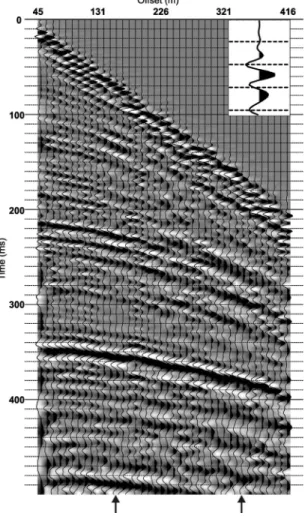
The data that we analyze consist of a 3⫻3 grid of CMP gathers extracted from a 3D survey. The survey was acquired using single explosive sources and single multicomponent digital receivers. The source and receiver spacing were 20 m, resulting in a 10-⫻10-m bin size. We apply minimal processing to the seismic data so as to avoid introducing lateral and temporal changes to the spectrum. Re-fraction and residual statics are applied, along with trace edits and a trapezoidal共10–20–120–180 Hz兲band-pass filter. To improve the signal-to-noise ratio, the CMPs are formed into a single stacked su-pergather. The offset range is restricted to 416 m, which provides 40 traces of data to a maximum offset-to-depth ratio of approximately 1.2. The final CMP supergather is shown in Figure9.
The reflection that we analyze has a zero-offset time of 324 ms, which is near the base of the zone of interest. Rather than use NMO-corrected data, we calculate the hyperbolic traveltimes using the stacking velocity field. Then we shift the center of the analysis along this curve, thereby avoiding the need to apply an NMO stretch cor-rection to the spectra. For a reference wavelet, we use the direct ar-rival from a near-offset trace. Because the data are acquired with point sources and receivers, there are no directivity effects on the spectrum to consider共Hustedt and Clark, 1999兲.
Results
We test first the stability of the natural log spectral ratio slopesA with the choice of regression bandwidth. The bandwidth-dependent slopes of a near共159-m兲and far共350-m兲offset are shown in Figure
10, in which for consistency, the data have been scaled to show 1/Qe. This analysis shows results that are consistent with the synthetic ex-periments. Specifically, for the far-offset example, the variable-win-dow transforms significantly extend the lower bandwidth frequency that produces a uniform 1/Qeestimate. For the near-offset case, the fixed-window transforms show an abrupt change in 1/Qeas the low-er frequency is increased, whlow-ereas the variable-window transforms have a much more gradual change.
Figure 9. CMP supergather used in the QVO analysis. An enlarge-ment of the reference wavelet is shown, and the offsets analyzed in Figure10are indicated by arrows. A 100-ms automatic gain control and a top mute have been applied for display purposes.
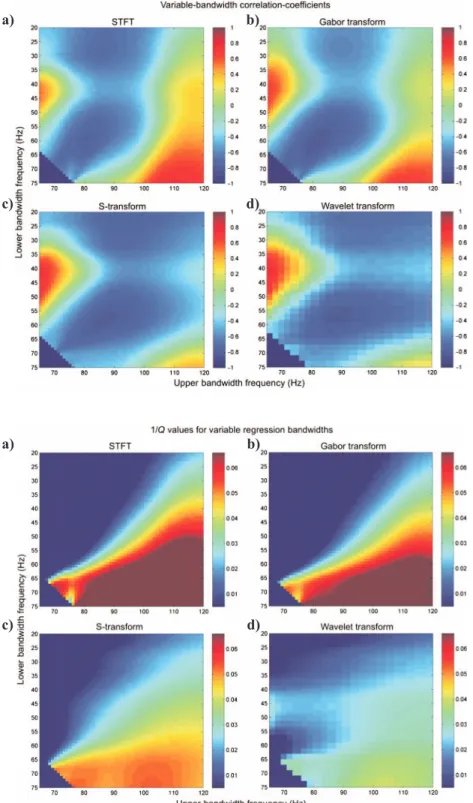
Because attenuation increases with traveltime, the relationship betweenAand⌬tis expected to be linear with a negative slope. In re-ality, the measurements fluctuate about this trend because of noise in the data, spectral interference, and apparent attenuation effects. To quantify how closely the measurements ofAand⌬tfollow the theo-retical behavior, we calculate the correlation coefficient. Given two variables, the correlation coefficient measures the degree to which they are related linearly. The values range between minus one and one corresponding to a perfect negative and positive correlation, re-spectively, whereas a value of zero indicates uncorrelated data共 Tay-lor, 1997兲. Figure11shows the correlation coefficients derived for the four transforms, and these data show thatAand⌬thave a
stron-ger correlation when measured by the variable-window transforms. These transforms also extend the bandwidth range in which this ex-pected behavior is observed.
Finally, Figure12shows the bandwidth dependency of the zero-offset 1/Qeestimate from theAversus⌬tregression. This result clearly shows that the variable-window transforms produce 1/Qe es-timates that are more robust than their fixed-window counterparts. Furthermore, the 1/Qevalues obtained are consistent with the type of geology investigated.Macrides and Kanasewich共1987兲, for exam-ple, use a crosswell experiment to find a value of 1/Qe⳱0.03 in un-consolidated heavy-oil reservoirs. Although this does not account for attenuation in the overburden, the findings are consistent with our measurements.
DISCUSSION
A single estimate of frequency-dependent 1/Qscfor a transmitted pulse is more accurate and has less uncertainty when made with a time-fre-quency transform that uses a variable-length time window instead of a fixed-length time window. This is shown by the statistical properties dis-played in Figure3. Similarly, when estimating a frequency-independent 1/Qefor both a synthetic and a real data reflection experiment, the vari-able-window transforms produce results that are more robust with respect to the choice of regres-sion bandwidth.
These observations arise because the variable-window transforms reduce the extent of the spec-tral fluctuations for two reasons. First, at high fre-quencies, at which typically more energy is scat-tered to the coda, there is an increase in the degree of nonstationarity in the data. The variable time windows use shorter time windows to analyze the high frequencies, so that the primary arrival is better isolated from the coda. This can be seen in Figure2, in which at higher frequencies, the spec-trum of the primary arrival is more distinct from the spectrum of the coda for variable-window transforms. Although the variable windows iso-late high frequencies as noted, they also include a larger portion of coda at lower frequencies. This is not detrimental, because共1兲only small amounts of low-frequency energy are in the coda as a result of the nature of the scattering and共2兲in a given time window, the variability of attenua-tion for lower frequencies is less than that for higher frequencies because of the reduced num-ber of wavelengths present.
The second reason behind the reduction of fluctuations also is related to window size. Be-cause of the Gabor uncertainty principle共Hall, 2006兲, as the time window becomes shorter, the effective frequency window increases in size. This means that there is an increased spectral av-eraging for the shorter windows, and any rapid fluctuations in the spectrum are smoothed out. Of course, the converse is true also, namely, that Figure 10. The 1/Qevalues for the near offset trace共left side兲and far offset trace共right
side兲, estimated over a range of bandwidths. At both trace offsets, the variable-window transforms共lower half兲increase the number of bandwidth choices that produce a stable 1/Qeestimate.
there is higher spectral resolution for the longer time windows at low frequencies.
Although it is possible to isolate the coda from the signal by using a shorter window length for the fixed-window transforms, this is not an ideal solution for broadband data. Figure5shows that the fluctua-tions about the theoretical value are reduced at higher frequencies, but the minimum frequency that can be measured properly increases also. This makes short windows detrimental for data consisting of a large frequency range. The variable-window transforms do not face
this problem, as they maintain a window length that is proportional to the period being analyzed.
The small differences between the results of the S-transform and wavelet transform demonstrate why it is more significant to compare classes of transforms, rather than the individual transforms them-selves. Small changes in the transform parameters or in the data be-ing analyzed can create situations in which either variable-window transform will show a small benefit over the other. Nevertheless, we prefer the S-transform over the wavelet transform because it
produc-c)
a)
d)
b)
Figure 11. Correlation coefficient plots betweenA and⌬tfor the共a兲STFT,共b兲Gabor transform,共c兲 S-transform, and共d兲wavelet transform. The theoreti-cal relationship results in a value ofⳮ1, and共c兲and 共d兲more closely approach this value over a larger choice of bandwidths.
a)
c)
b)
d)
Figure 12. The final 1/Qeestimates from the QVO method. As with previous results, estimates of the 共a兲STFT and共b兲Gabor transform are less stable than the共c兲S-transform and共d兲wavelet-transform measurements.
es spectral estimates as a function of frequency rather than scale, and because it preserves the time reference of the data’s phase informa-tion共Stockwell et al., 1996兲.
CONCLUSIONS
We have conducted two experiments to test what difference the choice of time-frequency transform makes when measuring seismic attenuation. We investigated two classes of transforms, those with fixed time windows and those with systematically varying time win-dows, in the context of measuring a frequency-dependent 1/Qsc caused by multiple scattering, and a frequency-independent effec-tive 1/Qefrom a linear regression of natural log spectral ratios versus frequency.
We have shown that the time-frequency transform used to calcu-late the spectrum of a transmitted wave influences the precision and accuracy of attenuation estimates. The S-transform and continuous wavelet transform decrease the variability of the attenuation esti-mate, specifically at the high and low ends of the spectrum. For high-er frequencies, the variability is reduced for two reasons:共1兲the pri-mary arrival is isolated from the coda by the shorter time windows used for higher frequencies; and共2兲the shorter window results in spectral averaging, thereby reducing the influence of spectral fluctu-ations such as notches and peaks. At the low-frequency end, im-provements are the results of proper amplitude determination by maintaining an adequate signal sample for each period.
Variable-window transforms also improve the robustness of a fre-quency-independent effective 1/Qeestimate obtained using a linear regression of natural log spectral ratios versus frequency. This offers more flexibility in the choice of bandwidth used for the regression. The increased robustness is seen in the analysis of a real data set, in which attenuation measurements across multiple offsets more close-ly follow an expected linear behavior with traveltime when they are made with variable-window transforms instead of fixed-window transforms. These measurements led to a determination of 1/Qethat is consistent with previously measured values. We therefore find that variable-window transforms, such as the S-transform and wavelet transform, offer distinct benefits for seismic attenuation analysis, in cases when a nonstationary signal must be evaluated.
ACKNOWLEDGMENTS
Funding for this research was kindly provided by Nexen Inc. We also thank Nexen Inc. and OPTI Canada Inc. for providing the well-log and seismic data for our analysis. In addition, discussions with Andrew Carter on attenuation, and input from Matt Hall and an anonymous reviewer, are greatly appreciated.
REFERENCES
Aki, K., and P. G. Richards, 2002, Quantitative seismology, 2nd ed.: Univer-sity Science Books.
Bracewell, R., 1978, The Fourier transform and its applications, 2nd ed.: McGraw-Hill Inc.
Carmona, R., W. Hwang, and B. Torresani, 1998, Practical time-frequency analysis: Gabor and wavelet transforms with an implementation in S: Aca-demic Press.
Carter, A. J., 2003, Seismic wave attenuation from surface seismic reflection surveys — An exploration tool?: Ph.D. thesis, University of Leeds. Castagna, J. P., and S. Sun, 2006, Comparison of spectral decomposition
methods: First Break,24, 75–79.
Chakraborty, A., and D. Okaya, 1995, Frequency-time decomposition of seismic data using wavelet-based methods: Geophysics,60, 1906–1916. Clark, R. A., A. J. Carter, P. C. Nevill, and P. M. Benson, 2001, Attenuation
measurements from surface seismic data — Azimuthal variation and time-lapse case studies: 63rd Conference and Technical Exhibition, EAGE, Ex-panded Abstracts, L-28.
Dasgupta, R., and R. A. Clark, 1998, Estimation ofQfrom surface seismic reflection data: Geophysics,63, 2120–2128.
Daubechies, I., 1992, Ten lectures on wavelets: Society for Industrial and Ap-plied Mathematics.
Dietrich, M., 1988, Modeling of marine seismic profiles in thet-xand-p do-mains: Geophysics,53, 453–465.
Dvorkin, J., and A. Nur, 1993, Dynamic poroelasticity — A unified model with the squirt and the Biot mechanisms: Geophysics,58, 524–533. Hall, M., 2006, Resolution and uncertainty in spectral decomposition: First
Break,24, 43–47.
Harris, F. J., 1978, Use of windows for harmonic analysis with discrete Fouri-er transform: Proceedings of the IEEE,66, 51–83.
Hauge, P. S., 1981, Measurements of attenuation from vertical seismic pro-files: Geophysics,46, 1548–1558.
Hustedt, B., and R. A. Clark, 1999, Source/receiver array directivity effects on marine seismic attenuation measurements: Geophysical Prospecting, 47, 1105–1119.
Johnston, D. H., M. N. Toksoz, and A. Timur, 1979, Attenuation of seismic waves in dry and saturated rocks: II — Mechanisms: Geophysics,44, 691– 711.
Kaderali, A., M. Jones, and J. Howlett, 2007, White Rose seismic with well data constraints: A case history: The Leading Edge,26, 742–754. Li, H., W. Zhao, H. Cao, F. Yao, and L. Shao, 2006, Measures of scale based
on the wavelet scalogram with applications to seismic attenuation: Geo-physics,71, no. 5, V111–V118.
Luh, P. C., 1993, Wavelet attenuation and bright-spot detection,inJ. P. Casta-gna and M. M. Backus, eds., Offset-dependent reflectivity: Theory and practice of AVO analysis: Investigations in Geophysics, 8, 190–198. Macrides, C. G., and E. R. Kanasewich, 1987, Seismic attenuation and
Pois-son’s ratios in oil sands from crosshole measurements: Journal of the Ca-nadian Society of Exploration Geophysicists,23, 46–55.
Mallat, S. G., and Z. F. Zhang, 1993, Matching pursuits with time-frequency dictionaries: IEEE Transactions on Signal Processing,41, 3397–3415. Maultzsch, S., M. Chapman, E. Liu, and X.-Y. Li, 2007, Modelling and
anal-ysis of attenuation anisotropy in multi-azimuth VSP data from the Clair field: Geophysical Prospecting,55, 627–642.
O’Doherty, R. F., and N. A. Anstey, 1971, Reflections on amplitudes: Geo-physical Prospecting,19, 430–458.
Reid, F. J. L., P. H. Nguyen, C. MacBeth, R. A. Clark, and I. Magnus, 2001,Q
estimates from north sea VSPs: 71st Annual International Meeting, SEG, Expanded Abstracts, 440–443.
Rioul, O., and M. Vetterli, 1991, Wavelets and signal processing: IEEE Sig-nal Processing Magazine, 1991, 14–38.
Sams, M. S., J. P. Neep, M. H. Worthington, and M. S. King, 1997, The mea-surement of velocity dispersion and frequency-dependent intrinsic attenu-ation in sedimentary rocks: Geophysics,62, 1456–1464.
Schoenberger, M., and F. K. Levin, 1974, Apparent attenuation due to intra-bed multiples: Geophysics,39, 278–291.
——–, 1978, Apparent attenuation due to intrabed multiples, II: Geophysics, 43, 730–737.
Shapiro, S. A., and H. Zien, 1993, The O’Doherty-Anstey formula and local-ization of seismic waves: Geophysics,58, 736–740.
Sinha, S., P. S. Routh, P. D. Anno, and J. P. Castagna, 2005, Spectral decom-position of seismic data with continuous-wavelet transform: Geophysics, 70, no. 6, P19–P25.
Spencer, T. W., C. M. Edwards, and J. R. Sonnad, 1977, Seismic-wave atten-uation in nonresolvable cyclic stratification: Geophysics,42, 939–949. Spencer, T. W., J. R. Sonnad, and T. M. Butler, 1982, SeismicQ—
Stratigra-phy or dissipation: GeoStratigra-physics,47, 16–24.
Stockwell, R. G., L. Mansinha, and R. P. Lowe, 1996, Localization of the complex spectrum: The S transform: IEEE Transactions on Signal Pro-cessing,44, 998–1001.
Tai, S., D. Han, and J. P. Castagna, 2006, Attenuation estimation with contin-uous wavelet transforms: 76th Annual International Meeting, SEG, Ex-panded Abstracts, 1933–1937.
Taylor, J. R., 1997, An introduction to error analysis: The study of uncertain-ties in physical measurements, 2nd ed.: University Science Books. Tonn, R., 1991, The determination of the seismic quality factorQfrom VSP
data — A comparison of different computational methods: Geophysical Prospecting,39, 1–27.
Toverud, T., and B. Ursin, 2005, Comparison of seismic attenuation models using zero-offset vertical seismic profiling共VSP兲data: Geophysics,70, no. 2, F17–F25.
van der Baan, M., 2001, Acoustic wave propagation in one-dimensional ran-dom media: The wave localization approach: Geophysical Journal Inter-national,145, 631–646.
van der Baan, M., J. Wookey, and D. Smit, 2007, Stratigraphic filtering and source penetration depth: Geophysical Prospecting,55, 679–684. Wang, Y. H., 2002, A stable and efficient approach of inverseQfiltering:
Geophysics,67, 657–663.
——–, 2007, Seismic time-frequency spectral decomposition by matching pursuit: Geophysics,72, no. 1, V13–V20.
Winkler, K. W., and A. Nur, 1982, Seismic attenuation — Effects of pore flu-ids and frictional sliding: Geophysics,47, 1–15.