A Comparison of Estimation Methods for Vector Autoregressive Moving-Average Models

Full text

(1)EUI Working Papers ECO 2007/12. A Comparison of Estimation Methods for Vector Autoregressive Moving-Average Models. Christian Kascha.

(2)

(3) EUROPEAN UNIVERSITY INSTITUTE. DEPARTMENT OF ECONOMICS. A Comparison of Estimation Methods for Vector Autoregressive Moving-Average Models CHRISTIAN KASCHA. EUI Working Paper ECO 2007/12.

(4) This text may be downloaded for personal research purposes only. Any additional reproduction for other purposes, whether in hard copy or electronically, requires the consent of the author(s), editor(s). If cited or quoted, reference should be made to the full name of the author(s), editor(s), the title, the working paper or other series, the year, and the publisher. The author(s)/editor(s) should inform the Economics Department of the EUI if the paper is to be published elsewhere, and should also assume responsibility for any consequent obligation(s). ISSN 1725-6704. © 2007 Christian Kascha Printed in Italy European University Institute Badia Fiesolana I – 50014 San Domenico di Fiesole (FI) Italy http://www.eui.eu/ http://cadmus.eui.eu/.

(5) A Comparison of Estimation Methods for Vector Autoregressive Moving-Average Models∗ Christian Kascha† March 2007. Abstract Classical Gaussian maximum likelihood estimation of mixed vector autoregressive moving-average models is plagued with various numerical problems and has been considered difficult by many applied researchers. These disadvantages could have led to the dominant use of vector autoregressive models in macroeconomic research. Therefore, several other, simpler estimation methods have been proposed in the literature. In this paper these methods are compared by means of a Monte Carlo study. Different evaluation criteria are used to judge the relative performances of the algorithms.. JEL classification: C32, C15, C63 Keywords: VARMA Models, Estimation Algorithms, Forecasting. ∗. I would like to thank Helmut Lütkepohl and Anindya Banerjee for helpful comments and discussion. European University Institute, Department of Economics, Via della Piazzuola 43, 50133 Firenze, Italy; E-mail: christian.kascha@eui.eu. †.

(6) 1. Introduction. Although vector autoregressive moving-average (VARMA) models have theoretical and practical advantages compared to simpler vector autoregressive (VAR) models, VARMA models are rarely used in applied macroeconomic work. One likely reason is that the estimation of these models is considered difficult by many researchers. While Gaussian maximum likelihood estimation is theoretically attractive, it is plagued with various numerical problems. Therefore, simpler estimation algorithms have been proposed in the literature that, however, have not been compared systematically. In this paper some prominent estimation methods for VARMA models are compared by means of a Monte Carlo study. Different evaluation criteria such as the accuracy of point forecasts or the accuracy of the estimated impulse responses are used to judge the algorithms’ performance. I focus on sample lengths and processes that could be considered typical for macroeconomic applications. The problem of estimating VARMA models received a lot of attention for several reasons. While most economic relations are intrinsically nonlinear, linear models such as VARs or univariate autoregressive moving-average (ARMA) models have proved to be successful in many circumstances. They are simple and analytically tractable, while capable of reproducing complex dynamics. Linear forecasts often appear to be more robust than nonlinear alternatives and their empirical usefulness has been documented in various studies (e.g. Newbold & Granger 1974). Therefore, VARMA models are of interest as generalizations of successful univariate ARMA models. In the class of multivariate linear models, pure VARs are currently dominating in macroeconomic applications. These models have some drawbacks which could be overcome by the use of the more general class of VARMA models. First, VAR models may require a rather large lag length in order to describe a series “adequately”. This means a loss of precision because many parameters have to be estimated. The problem could be avoided by using VARMA models that may provide a more parsimonious description of the data generating process (DGP). In contrast to the class of VARMA models, the class of VAR models is not closed under linear transformations. For example, a subset of variables generated by a VAR process. 2.

(7) is typically generated by a VARMA, not by a VAR process. The VARMA class includes many models of interest such as unobserved component models. It is well known that linearized dynamic stochastic general equilibrium (DSGE) models imply that the variables of interest are generated by a finite order VARMA process. Fernández-Villaverde, Rubio-Ramı́rez & Sargent (2005) show formally how DSGE models and VARMA processes are linked. Also Cooley & Dwyer (1998) claim that modelling macroeconomic time series systematically as pure VARs is not justified by the underlying economic theory. In sum, there are a number of theoretical reasons to prefer VARMA modelling to VAR modelling. However, there are also some complications that make VARMA modelling more difficult. First, VARMA representations are not unique. That is, there are typically many parameterizations that can describe the same DGP (see Lütkepohl 2005). Therefore, a researcher has to choose first an identified representation. In any case, an identified VARMA representation has to be specified by more integer-valued parameters than a VAR representation that is determined just by one parameter, the lag length. Thus, the search for an identified VARMA model is more complex than the specification of a VAR model. This aspect introduces additional uncertainty in the specification stage, although specification procedures for VARMA models do exist which could be used in a completely automatic way (Hannan & Kavalieris 1984b, Poskitt 1992). An identified representation, however, is needed for consistent estimation. Apart from a more involved specification stage, the estimation stage is also affected by the identification problem. The literature on estimation of VARMA models focussed on maximum likelihood methods which are asymptotically efficient (e.g. Hillmer & Tiao 1979, Mauricio 1995). However, the maximization of the Gaussian likelihood is not a trivial task. Numerical problems arise in the presence of nearly not-identified models, multiple equilibria and nearly non-invertible models. In high-dimensional, sparse systems maximum likelihood estimation may become even infeasible. In the specification stage one usually has do examine many different models which turn out not to be identified ex-post. For these reasons several other estimation algorithms have been proposed in the literature. For example, Koreisha & Pukkila (1990) proposed a generalized least squares procedure. Kapetanios (2003) suggested an iterative least squares algorithm that uses only ordinary least. 3.

(8) squares regressions at each iteration. Recently, subspace algorithms for state space systems, an equivalent representation of a VARMA process, have become popular also among econometricians. Examples are the algorithms of Van Overschee & DeMoor (1994) or Larimore (1983).1 While there are nowadays several possible estimation methods available, it is not clear which methods are preferable under which circumstances. In this study some of these methods are compared by means of a Monte Carlo Study. Instead of focussing only on the accuracy of the parameter estimates, I consider the use of the estimated VARMA models. After all, a researcher might be rather interested in the accuracy of the generated forecasts or the precision of the estimated impulse response function than in the actual parameter estimates. I conduct Monte Carlo simulations for four different DGPs with varying sample lengths and parameterizations. Five different simple algorithms are used and compared to maximum likelihood estimation and two benchmark VARs. The algorithms are a simple two-stage least squares algorithm, the iterative least squares procedure of Kapetanios (2003), the generalized least squares procedure of Koreisha & Pukkila (1990), a three-stage least squares procedure based on Hannan & Kavalieris (1984a) and the CCA subspace algorithm by Larimore (1983). The obtained results suggest that the algorithm of Hannan & Kavalieris (1984a) is the only algorithm that reliably outperforms the other algorithms and the benchmark VARs. However, the procedure is technically not very reliable in that the algorithm very often yields estimated models which are not invertible. Therefore, the algorithm would have to be improved in order to make it an alternative tool for applied researchers. The rest of the paper is organized as follows. In section 2 stationary VARMA processes and state space systems are introduced and some identified parameterizations are presented. In section 3 the different estimation algorithms are described. The setup and the results of the Monte Carlo study are presented in section 4. Section 5 concludes. 1. See also the survey of Bauer (2005b).. 4.

(9) 2. Stationary VARMA Processes. I consider linear, time-invariant, covariance - stationary processes (yt )t∈Z of dimension K that allow for a VARMA(p, q) representation of the form. A0 yt = A1 yt−1 + . . . + Ap yt−p + M0 ut + M1 ut−1 + . . . + Mq ut−q. (1). for t ∈ Z, p, q ∈ N0 . The matrices A0 , A1 , . . . , Ap and M0 , M1 , . . . , Mq are of dimension (K × K). The term ut represents a K-dimensional white noise sequence of random variables with mean zero and nonsingular covariance matrix Σ. In principle, equation (1) should contain an intercept term and other deterministic terms in order to account for random series with non-zero mean and/or seasonal patterns. This has not been done here in order to simplify the exposition of the basic properties of VARMA models and the related estimation algorithms. For most of the algorithms discussed later, it is assumed that the mean has been subtracted prior to estimation. We will also abstract from issues such as seasonality. As will be seen later, we consider models of the form (1) such that A0 = M0 and A0 , M0 are non-singular. This does not imply a loss of generality as long as no variable can be written as a linear combination of the other variables (Lütkepohl 2005). It can be shown that any stationary and invertible VARMA process can then be expressed in the above form. Let L denote the lag-operator, i.e. Lyt = yt−1 for all t ∈ Z, A(L) = A0 − A1 L − . . . − Ap Lp and M (L) = M0 + M1 L + . . . + Mq Lq . We can write (1) more compactly as A(L)yt = M (L)ut , t ∈ Z.. (2). VARMA processes are stationary and invertible if the roots of these polynomials are all outside the unit circle. That is, if. |A(z)| 6= 0, |M (z)| 6= 0 for z ∈ C, |z| ≤ 1. is true. These restrictions are important for the estimation and for the interpretation of VARMA models. The first condition ensures that the process is covariance-stationary and 5.

(10) has an infinite moving-average or canonical moving-average representation. yt =. ∞ X. Φi ut−i = Φ(L)ut ,. (3). i=0. where Φ(L) = A(L)−1 M (L). If A0 = M0 is assumed, then Φ0 = IK where IK denotes an identity matrix of dimensions K. The second condition ensures the invertibility of the process, in particular the existence of an infinite autoregressive representation. yt =. ∞ X. Πi yt−i + ut ,. (4). i=1. where A0 = M0 is assumed and Π(L) = IK −. P∞. i i=1 Πi L. = M (L)−1 A(L). This representation. indicates, why a pure VAR with a large lag length might approximate processes well that are actually generated by a VARMA system. It is well known that the representation in (1) is generally not identified unless special restrictions are imposed on the coefficient matrices (Lütkepohl 2005). Precisely, all pairs of polynomials A(L) and M (L) which lead to the same canonical moving-average operator Φ(L) = A(L)−1 M (L) are equivalent. However, uniqueness of the pair (A(L), M (L)) is required for consistent estimation. The first possible source of non-uniqueness is that there are common factors in the polynomials that can be canceled out. For example, in a VARMA(1, 1) system such as. (IK − A1 L)yt = (IK + M1 L)ut the autoregressive and the moving-average polynomial cancel out against each other if A1 = −M1 . In order to ensure a unique representation we have to require that there are no common factors in both polynomials, that is A(L) and M (L) have to be left-coprime. This property may be defined by introducing the matrix operator [A(L), M (L)] and calling it left-coprime if the existence of operators D(L), Ā(L) and M̄ (L) satisfying. D(L)[Ā(L), M̄ (L)] = [A(L), M (L)]. 6. (5).

(11) implies that D(L) is unimodular.2 A polynomial matrix D(L) is called unimodular if its determinant, |D(L)|, is a nonzero constant that does not depend on L. Then D(L) can only be of finite order having a finite order inverse. This condition ensures just that a representation is chosen for which further cancelation is not possible. Still, the existence of many unimodular operators satisfying equation (5) cannot generally be ruled out. To obtain uniqueness of the autoregressive and moving-average polynomials we have to impose further restrictions ensuring that the only feasible operator satisfying the above equation is D(L) = IK . Therefore, different representations have been proposed in the literature (Hannan & Deistler 1988, Lütkepohl 2005). These representations impose particular restrictions on the coefficient matrices that make sure that for a given process there is exactly one representation in the set of considered representations. We present two identified representations which are used later. A VARMA(p, q) is in final equations form if it can be written as α(L)yt = (I + M1 + . . . + Mq Lq )ut , where α(L) := 1 − α1 L − . . . − αp Lp is a scalar operator with αp 6= 0. The moving-average polynomial is unrestricted apart from M0 = IK . It can be shown that this representation is uniquely identified provided that p is minimal (Lütkepohl 2005). A disadvantage of the final equations form is that it requires usually more parameters than other representations in order to represent the same stochastic process and thus might not be the most efficient representation. The Echelon representation is based on the Kronecker index theory introduced by Akaike (1974). A VARMA representation for a K-dimensional series yt is completely described by K Kronecker indices or row degrees, (p1 , . . . , pK ). Denote the elements of A(L) and M (L) as A(L) = [αki (L)]ki and M (L) = [mki (L)]ki . The Echelon form imposes zero-restrictions 2. [A, B] denotes a matrix composed horizontally of two matrices A and B.. 7.

(12) according to. αkk (L) = 1 − αki (L) = − mki (L) =. pk X. αkk,j Lj ,. j=1 pk X. αki,j Lj , for k 6= j,. j=pk −pki +1 p k X mki,j Lj with j=0. M0 = A0 ,. for k, i = 1, . . . , K. The numbers pki are given by. pki =.    min{pk + 1, pi }, if k ≥ i   min{pk , pi },. k, i = 1, . . . , K,. if k < i. and denote the number of free parameters in the polynomials, αki (L), k 6= i. Again, it can be shown that this representation leads to identified parameters (Hannan & Deistler 1988). In this setting, a measure of the overall complexity of the multiple series can be given by the P McMillian degree kj=1 pj which is also the dimension of the corresponding state vector in a state space representation. Note that the Echelon Form with equal Kronecker indices, i.e. p1 = p2 = . . . = pK , corresponds to a standard unrestricted VARMA representation. This is one of the most promising representations, from a theoretical point of view, since it often leads to more parsimonious models than other representations. There is also another representation of the same process which is algebraically equivalent. Every process that satisfies (1) can also be written as a state space model of the form. xt+1 = Axt + But ,. (6). yt = Cxt + ut , where the vector xt is the so-called state vector of dimension (n×1) and A (n×n), B (n×K), C (K × n) are fixed coefficient matrices. Generally, the state xt is not observed. Processes that satisfy (6) can be shown to have a VARMA representation (see, e.g., Aoki 1989, Hannan & Deistler 1988). In the appendix it is illustrated how a VARMA model can be written in 8.

(13) state space form and how a state space model can define a VARMA model. Also the state space representation is not identified unless restrictions on the parameter matrices are imposed. Analogously to the VARMA case, we first have to rule out overparametrization by requiring that the order of the state vector, n, is minimal. Still, this does not determine a unique set (A, B, C) for a given process. To see this, consider multiplying the state vector by a nonsingular matrix T and define a new state vector st := Txt . The redefinition of the state leads to another state space representation given by st+1 = TAT−1 st + TBut , yt = CT−1 st + ut . Thus, the problem is to pin down a basis for the state xt . There are various canonical parameterizations, among them parameterizations based on Echelon canonical forms. We briefly discuss here balanced canonical forms, in particular stochastic balancing, because it is used later in one of the estimation algorithms. The discussion on stochastic balancing is based on Desai, Pal & Kirkpatrick (1985) and the introduction in Bauer (2005a). Define the observability matrix O := [C 0 , A0 C 0 , (A2 )0 C 0 , . . .]0 and the matrix K := [B, (A − BC)B, (A − BC)2 B, . . .]. The unique parametrization is defined in terms of these matrices. Define as well an infinite vector of future observations as Yt+ := 0 , . . .)0 and an infinite vector of past observations as Y − := (y 0 , y 0 , . . .)0 . Define (yt0 , yt+1 t t−1 t−2. analogously the vector of future residuals, Ut+ . Note that from (6) we can represent the state as a function of all past observations as xt = KYt− , provided that the eigenvalues of (A − BC) are less than one in modulus. The covariance 0 matrix of the state vector is therefore given by E[xt x0t ] = KE[Yt− (Yt− )0 ]K0 = KΓ− ∞ K , where − − 0 Γ− ∞ := E[Yt (Yt ) ]. Given a state space system as in (6), there is also another representation. 9.

(14) which is called backward innovation model zt = A0 zt+1 + N ft , yt = M 0 zt+1 + ft , where time “runs backwards” and A is as in (6) and N (n × K), M (n × K) are functions 0 ]. The error f can be interpreted as the one-step of (A, B, C), in particular M = E[xt yt−1 t. ahead forecast error from predicting yt given future observations. One can show that the −1 variance of the backward state is given by E[zt zt0 ] = O0 (E[Yt+ (Yt+ )0 ])−1 O = O0 (Γ+ ∞ ) O, + + 0 where Γ+ ∞ := E[Yt (Yt ) ].. Equipped with these definitions, we say that (A, B, C) and Σ is a stochastically balanced system if E[xt x0t ] = E[zt zt0 ] = diag(σ1 , . . . , σn ), with 1 > σ1 ≥ σ2 ≥ . . . ≥ σn > 0. Also stochastically balanced systems are not unique. Uniqueness can however be obtained by determining the matrices O and K by means of the identification restrictions implicit in the singular value decomposition (SVD) for a given covariance sequence. For doing so, introduce the Hankel matrix of autocovariances of yt   γ(1) γ(2) γ(3) . . .     γ(2) γ(3)    H := E[Yt+ (Yt− )0 ] =  ,   γ(3)     .. . 0 ], j = 1, 2, . . . are the covariance matrices of the process y . Using the where γ(j) := E[yt yt−j t. relation H = OKΓ− ∞ , a stochastically balanced representation can be obtained by using the SVD of h i0 −1/2 − −1/2 (Γ+ ) H (Γ ) = Un Sn Vn0 . ∞ ∞ 1/2. 1/2 U S Setting O = (Γ+ n n ∞). 1/2. −1/2 , the associated system is in balanced and K = Sn Vn0 (Γ− ∞). 10.

(15) form with E[xt x0t ] = E[zt zt0 ] = Sn .3 From the definition of the parametrization one can see that it is not easy to incorporate prior knowledge of parameter restrictions. While the VARMA and the state space representation are equivalent in an algebraic sense, they lead to other estimation techniques and therefore differ in a statistical sense. These models have become popular because of their conceptional simplicity and because they allow for estimation algorithms, namely so-called subspace methods, that possess very good numerical properties. See also Deistler, Peternell & Scherrer (1995) and Bauer (2005b) for some of the properties of subspace algorithms. It is claimed that these methods are very successful in estimating multivariate linear systems. Therefore, subspace methods are also considered as potential competitors to estimation techniques which rely on the more standard VARMA representation.. 3. Description of Estimation Methods. In the following, a short description of the examined algorithms is given. Obviously, one cannot consider each and every existing algorithm but only a few popular algorithms. The hope is that the performance of these algorithms indicate how their variants would work. Throughout it is assumed that the data has been mean-adjusted prior to estimation. In the following, I do not distinguish between raw data and mean-adjusted data for notational ease. Most of the algorithms are discussed based on the general representation (1) and throughout it is assumed that restrictions are imposed on the parameter vector of the VARMA model. That is, the coefficient matrices are assumed to be restricted according to the final equations form or the Echelon form. I adopt the following notation. The observed sample is y1 , y2 , . . . , yT . I denote the vector of total parameters by β (K 2 (p+q)×1) and the vector of free parameters by γ. Let the dimension of γ be given by nγ . Let A := [A1 , . . . , Ap ] and M := [M1 , . . . , Mq ] be matrices collecting the autoregressive and moving-average coefficient matrices, respectively. Define. β := vec[IK − A0 , A, M], 3. The square root of a matrix X, Y = X 1/2 is defined such that Y Y 0 = X.. 11.

(16) where vec denotes the operator that transforms a matrix to a column vector by stacking the columns of the matrix below each other. This particular order of the free parameters allows to formulate many of the following estimation methods as standard linear regression problems. A0 is assumed to be either the identity matrix or to satisfy the restrictions imposed by the Echelon representation. To consider zero and equality restrictions on the parameters, define a ((K 2 (p + q)) × nγ ) matrix R such that β = Rγ.. (7). This notation is equivalent to the explicit formulation of restrictions on β such as Cβ = c for suitable matrices C and c. The above notation, however, is advantageous for the representation of the estimation algorithms. Two-Stage Least Squares (2SLS) This is the simplest method. The idea is to use the infinite VAR representation in (4) in order to estimate the residuals ut in a first step. In finite samples, a good approximation is a finite order VAR, provided that the process is of low order and the roots of the moving-average polynomial are not too close to unity in modulus. The first step of the algorithm consists of a preliminary long autoregression of the type. yt =. nT X. Πi yt−i + ut ,. (8). i=1. where nT is the lag length that is required to increase with the sample size, T . In the second (0). stage, the residuals from (8), ût , are plugged in (1). After rearranging (1), one gets (0). yt = (IK − A0 )[yt − ût ] + A1 yt−1 + . . . + Ap yt−p (0). (0). +M1 ût−1 + . . . + Mq ût−q + ut , where A0 = M0 has been used. Write the above equation compactly as (0). yt = [IK − A0 , A, M]Yt−1 + ut ,. 12. (9).

(17) where. (0). Yt−1.   (0) (yt − ût )      yt−1      .   ..       :=  yt−p  .       û(0) t−1     ..   .     (0) ût−q. Collecting all observations we get Y = [IK − A0 , A, M]X (0) + U,. (10). where Y := [ynT +m+1 , . . . , yT ], U := [unT +m+1 , . . . , uT ] is the matrix of regression errors, (0). (0). X (0) := [YnT +m , . . . , YT −1 ] and m := max{p, q}. Thus, the regression is started at nT + m + 1. One could also start simply at m + 1, setting the initial errors to zero but we have decided not to do so. Vectorizing equation (10) yields 0. vec(Y ) = (X (0) ⊗ IK )Rγ + vec(U ), and the 2SLS estimator is defined as 0 e −1 )R]−1 R0 (X (0) ⊗ Σ e −1 )vec(Y ). γ̃ = [R0 (X (0) X (0) ⊗ Σ. (11). e is the covariance matrix estimator based on the residuals û(0) . The corresponding where Σ t estimated matrices are denoted by Ã0 , Ã1 , . . . , Ãp and M̃1 , M̃2 . . . , M̃q , respectively. Alter(0). natively, one may also plug in the estimated current innovation ût (0). regression error, say ξt , and regress yt − ût. in (9), define a new. (0). on Yt−1 . Existing Monte Carlo studies though. indicate that the difference between both variants is of minor importance (Koreisha & Pukkila 1989).. 13.

(18) For univariate and multivariate models different selection rules for the lag length of the initial autoregression have been proposed. For example, Hannan & Kavalieris (1984a) propose √ to select nT by AIC or BIC, while Koreisha & Pukkila (1990) propose choosing nT = T √ or nT = 0.5 T . In general, choosing a higher value for nT increases the risk of obtaining non-invertible or non-stationary estimated models (Koreisha & Pukkila 1990). Lütkepohl & √ Poskitt (1996) propose for multivariate, non-seasonal data a value between log T and T . √ Throughout the whole paper we employ nT = 0.5 T .4 Hannan-Kavalieris-Procedure (3SLS) This method adds a third stage to the procedure just described. It goes originally back to Durbin (1960) and has been introduced by Hannan & Kavalieris (1984a) for multivariate processes.5 It is a Gauss-Newton procedure to maximize the likelihood function conditional on yt = 0, ut = 0 for t ≤ 0 but its first iteration has been sometimes interpreted as a three-stage least squares procedure (Dufour & Pelletier (2004)). The method is computationally very easy to implement because of its recursive nature. Corresponding to the estimates of the 2SLS algorithm, new residuals, εt (K × 1), are formed. One step of the Gauss-Newton iteration is performed starting from these estimates. For this reason, matrices, ξt (K × 1), ηt (K × 1) and X̂t (K × nγ ) are calculated according to  εt = Ã0. −1. Ã0 yt − . ξt = Ã0. −1. − . ηt = Ã0. −1. − . X̂t = Ã0. −1. −. p X j=1. q X. M̃j εt−j  ,. j=1.  M̃j ηt−j + yt  ,. j=1 q X. . . M̃j ξt−j + εt  ,. j=1 q X. Ãj yt−j −. q X.  M̃j X̂t−j + (Ỹt0 ⊗ IK )R ,. j=1 4 Since this algorithm provides also starting values for other algorithms, it is quite important that the resulting estimated VARMA model is invertible. In case the initial estimate does not imply an invertible VARMA model, different lag lengths are tried in order to obtain an invertible model. If this procedure fails, c(L), is replace by M cλ (L) = M̂0 + λ(M c(L) − M̂0 ), λ ∈ (0, 1). the estimated moving-average polynomial, say M The latter case occurs in less than 0.1 % of the cases. 5 See also Hannan & Deistler (1988), sections 6.5, 6.7, for an extensive discussion.. 14.

(19) for t = 1, 2, . . . , T and yt = εt = ξt = ηt = 0K×1 and X̂t = 0K×nγ for t ≤ 0 and Ỹt is structured (0). as Yt. (0). with εt in place of ût . Given these quantities, we compute the 3SLS estimate as Ã γ̂ =. T X m+1. !−1 Ã 0 b −1 X̂t−1 X̂t−1 Σ t. T X. ! b −1 (εt + ηt − ξt ) , X̂t−1 Σ. m+1. b := T −1 P εt ε0t , m := max{p, q} as before and the estimated coefficient matrices are where Σ denoted by Â0 , Â1 , . . . , Âp and M̂1 , M̂2 , . . . , M̂q , respectively. While the 2SLS estimator is not asymptotically efficient, the 3SLS is, because it performs one iteration of a conditional maximum likelihood procedure starting from the estimates of the 2SLS procedure. Hannan & Kavalieris (1984b) showed consistency and asymptotic normality of these estimators. Dufour & Pelletier (2004) extend these results to even more general conditions. The Monte Carlo evidence presented by Dufour & Pelletier (2004) indicates that this estimator represents a good alternative to maximum likelihood in finite samples. It is possible to use this procedure iteratively, starting the above recursions in the second iteration with the newly obtained parameter estimates in γ̂ from the 3SLS procedure, and so on until convergence. Generalized Least Squares (GLS) Also this procedure has three stages. Koreisha & Pukkila (1990a) proposed this procedure for univariate ARMA models and Kavalieris, Hannan & Salau (2003) proved efficiency of the GLS estimates in this case. See also Flores de Frutos & Serrano (2002). The motivation is the same as for the 2SLS estimator. Given consistent estimates of the residuals, we can estimate the parameters of the VARMA representation by least squares. However, Koreisha & Pukkila (1990a) note that in finite samples the residuals are estimated with error. This implies that the actual regression error is serially correlated in a particular way due to the structure of the underlying VARMA process. The GLS procedure tries to take this into account. I consider a multivariate generalization of the same procedure. In the first stage, preliminary estimates of the innovations are obtained by a long autoregression as in (8). Koreisha & Pukkila (1990a) assume that the residuals obtained (0). from (8) estimate the true residuals up to an uncorrelated error term, ut = ût + ²t . If this. 15.

(20) expression is inserted in (1), one obtains. A0 yt =. p X. (0). Aj yt−j + A0 (ût + ²t ) +. j=1 (0). q X. (0). Mj ût−j + A0 ²t +. j=1 (0). yt − ût. (0). Mj (ût−j + ²t−j ),. j=1. yt = (IK − A0 )(yt − ût ) + +. q X. (0). = (I − A0 )(yt − ût ) +. p X j=1 q X. (0). Aj yt−j + ût Mj ²t−j ,. j=1 p X. Aj yt−j. j=1. +. q X. (0). Mj ût−j + ζt .. (12). j=1. As can be seen from these equations, the error term, ζt , in a regression of yt on its lagged (0). values and estimated residuals ût is not uncorrelated but is a moving-average process of P P order q, ζt = A0 ²t + qj=1 Mj ²t−j = ²̃t + qj=1 Mj A−1 0 ²̃t−j , where ²̃t := A0 ²t . Thus, a least squares regression in (12) is not efficient. Koreisha & Pukkila (1990a) propose the following three-stage algorithm to take the correlation structure of ζt into account. In the first stage the residuals are estimated using a long autoregression. In the second stage one estimates the (0). coefficients in (12) by ordinary least squares: Let zt := yt − ût. and Z := [znT +m+1 , . . . , zT ].. The second stage estimate is given analogously to the 2SLS final estimate by 0 γ̃˜ = [R0 (X (0) X (0) ⊗ IK )R]−1 R0 (X (0) ⊗ IK )vec(Z),. and the residuals are computed in the usual way, that is (0) 0 ˜ ˜ ζ̃t = zt − (Yt−1 ⊗ IK )Rγ̃.. The covariance matrix of these residuals, Σζ := E[ζt ζt0 ], is estimated as Σ̃ζ = T −1. P˜ ˜ 0 ζ̃t (ζ̃t ) .. From the relations ζt = A0 ²t + M1 ²t−1 + . . . + Mq ²t−q and Σζ = A0 Σ² A00 + . . . + Mq Σ² Mq0 one. 16.

(21) can retrieve Ã q !−1 X ˜ ˜ vec(Σ̃ζ ), (M̃i ⊗ M̃i ) vec(Σ̃² ) = i=0. ˜ are formed from the corresponding elements in γ̃. ˜ These estimates are then where the M̃ j used to build the covariance matrix of ζ = (ζn0 T +m+1 . . . ζT0 )0 . Let Φ := E[ζζ 0 ] and denote its estimate by Φ̂. In the third stage, we re-estimate (12) by GLS using Φ̂: 0 γ̃ˆ = [R0 (X (0) ⊗ IK )Φ̂−1 (X (0) ⊗ IK )R]−1 R0 (X (0) ⊗ IK )Φ̂−1 vec(Z).. In comparison to the 2SLS estimator the main difference lies in the GLS weighting with Φ̂−1 . Given γ̃ˆ one could calculate new estimates of the residuals ζt and update the estimate of the covariance matrix. Given these quantities one would obtain a new estimate of the parameter vector and so on until convergence.6 Iterative Least Squares (IOLS) The suggestion made by Kapetanios (2003) is simply to use the 2SLS algorithm iteratively. Denote the estimate of the 2SLS procedure by γ̃ (1) . We may obtain new residuals by 0. vec(Û (1) ) = vec(Y ) − (X (0) ⊗ IK )Rγ̃ (1) . Therefore, it is possible to set up a new matrix of regressors X (1) that is of the same structure (1). as X (0) but uses the newly obtained estimates of the residuals ût. in Û (1) . Generalized least. squares as in (11) in 0. vec(Y ) = (X (1) ⊗ IK )Rγ + vec(U ) yields a new estimate γ̃ (2) . Denote the vector of estimated residuals at the ith iteration by Û (i) . Then we iterate least squares regressions until ||Û (i−1) − Û (i) || < c according to some 6 The evidence given by Koreisha & Pukkila (1990a), however, suggests that further iterations do have a negligible effect. This is also the experience of the present author. The results presented here are therefore given for the first iteration of the GLS procedure.. 17.

(22) pre-specified number c. In contrast to the above-mentioned regression-based procedures, the IOLS procedure is iterative but the computational load is still minimal. Maximum Likelihood Estimation (MLE) The dominant approach to the estimation of VARMA models has been of course maximum likelihood estimation. Given a sample, y1 , ..., yT , the Gaussian likelihood conditional on initial values can be easily set up as. l(γ) =. T X. lt (γ). t=1. where 1 1 K log 2π − log |Σ| − u0t (γ)Σ−1 ut (γ), 2 2 2 ¡ −1 ut (γ) = M0 A0 yt − A1 yt−1 − . . . − Ap yt−p ¢ −M1 ut−1 (γ) − . . . − Mq ut−q (γ) . lt (γ) = −. The initial values for yt and ut are assumed to be fixed equal to zero (see Lütkepohl 2005). These assumptions introduce a negligible bias if the orders of the VARMA model are low and the roots of the moving-average polynomial are not close to the unit circle. In contrast, exact maximum likelihood estimation does consider the exact, unconditional likelihood that backcasts the initial values. The formulation of this procedure requires some considerable investment in notation and can be found for example in Reinsel (1993). Since processes with large moving-average eigenvalues are also investigated, exact maximum likelihood estimation is considered. The procedure is implemented using the time series package 4.0 in GAUSS. The algorithm is based upon the formulation of Mauricio (1995) and uses a modified Newtonalgorithm. The starting values are the true parameter values and therefore the results from the exact maximum likelihood procedure must be regarded as a benchmark than as a realistic estimation alternative. Subspace Algorithms (CCA) Subspace algorithms rely on the state space representation of a linear system. There are many ways to estimate a state space model, e.g., Kalman-. 18.

(23) based maximum likelihood methods and subspace identification methods such as N4SID of Van Overschee & DeMoor (1994) or the CCA method of Larimore (1983). In addition, many variants of the standard subspace algorithms have been proposed in the literature. I focus only on one subspace algorithm, the CCA algorithm. The algorithm is asymptotically equivalent to maximum likelihood and was previously found to be remarkably accurate in small samples and is likely to be well suited for econometric applications (see Bauer 2005b). The general motivation for the use of subspace algorithms lies in the fact that if we knew the unobserved state, xt , we could estimate the system matrices, A, B, C, by linear regressions as can be seen from the basic equations. xt+1 = Axt + But yt = Cxt + ut . Given knowledge of the state, estimates, Ĉ and ût , could be obtained by a regression of yt on xt and Â and B̂ could be obtained by a regression of xt+1 on xt and ût . Therefore, one obtains in a first step an estimate of the n-dimensional state, x̂t . This is analogous to the idea of a long autoregression in VARMA models that estimates the residuals in a first step that is followed by a least squares regression. Solving the state space equations, one can express the state as a function of past observations of yt and an initial state for some integer p > 0 as xt = (A − BC)p xt−p +. p−1 X (A − BC)i Byt−i−1 , i=0. − = (A − BC) xt−p + Kp Yt,p , p. (13). − 0 , . . . , y 0 ]0 . On the other where Kp = [B, (A − BC)B, . . . , (A − BC)p−1 B] and Yt,p = [yt−1 t−p. hand, one can express future observations as a function of the current state and future noise as. yt+j. j. = CA xt +. j−1 X. CAi But+j−i−1 + ut+j .. i=0. 19. (14).

(24) Therefore, at each t, the best predictor of yt+j is a function of the current state only, CAj xt , and thus the state summarizes in a certain sense all available information in the past up to time t. + 0 0 Define Yt,f = [yt0 , . . . , yt+f −1 ] for some integer f > 0 and formulate equation (14) for all + simultaneously. Combine these equations with (13) in order to observations contained in Yt,f. obtain + Yt,f. − + = Of Kp Yt,p + Of (A − BC)p xt−p + Ef Et,f. + = [u0t , . . . , u0t+f −1 ]0 and Ef is a function of the where Of = [C 0 , A0 C 0 , . . . , (Af −1 )0 C 0 ]0 , Et,f. system matrices. The above equation is central for most subspace algorithms. Note that if the maximum eigenvalue of (A−BC) is less than one in absolute value we have (A−BC)p ≈ 0 for large p. This condition is called the minimum phase assumption. This reasoning motivates an approximation of the above equation given by + Yt,f. − + = βYt,p + Nt,f. (15). + where β = Of Kp and Nt,f is defined by the equation. Most popular subspace algorithms. use this equation to obtain an estimate of β which is decomposed into Of and Kp . The identification problem is solved implicitly during this step. Different algorithms use these matrices differently to obtain an estimate of the state. Given an estimate of the state, the system matrices are recovered. For given integers n, p, f , the employed algorithm consists of the following steps : + − 1. Set up Yt,f and Yt,p and perform OLS in (15) using the available data to get an estimate. β̂f,p . 2. Compute the sample covariances. Γ̂+ f =. T −f +1 T −f +1 1 X 1 X + + 0 − − 0 Yt,f (Yt,f ) , Γ̂− = Yt,p (Yt,p ), p Tf,p Tf,p t=p+1. t=p+1. 20.

(25) where Tf,p = T − f − p + 1. 3. Given the dimension of the state, n, compute the singular value decomposition −1/2 1/2 (Γ̂+ β̂f,p (Γ̂− = Ûn Σ̂n V̂n0 + R̂n , p) f). where Σ̂n is a diagonal matrix that contains the n largest singular values and Ûn and V̂n are the corresponding singular vectors. The remaining singular values are neglected and the approximation error is R̂n . The reduced rank matrices are obtained as Ôf. 1/2 = [(Γ̂+ Ûn Σ̂1/2 n ], f). −1/2 K̂p = [Σ̂n1/2 V̂n0 (Γ̂− ]. p). − 4. Estimate the state as x̂t = K̂p Yt,p and estimate the system matrices using linear regres-. sions as described above. Although the algorithm looks quite complicated at first sight, it is actually very simple and is regarded to lead to numerically stable and accurate estimates. There are certain parameters which have to be determined before estimation. While the order of the system is given by the simulated process, the integers f, p have to be chosen deterministically or data-dependent. For example, Deistler et al. (1995) advocated choosing f = p = dpBIC for some d > 1, while in the paper of Bauer (2005a) f = p = 2pAIC is suggested, where pBIC and pAIC are the orders chosen by the BIC and AIC criterion for an autoregressive approximation, respectively. Here f = p = 2pAIC is employed.. 4. Monte Carlo Study. I compare the performance of the different estimation methods using a variety of measures that could reveal possible gains of VARMA modelling. Namely, the parameter estimation precision, the accuracy of point forecasts and the precision of the estimated impulse responses are compared. These measures are related. For instance, one would expect that an algorithm. 21.

(26) that yields accurate parameter estimates performs also well in a forecasting exercise. However, it is also known that simple univariate models such as an AR(1) can outperform much more general models or even the correct model in terms of forecasting precision. This phenomenon is simply due to the limited information in small samples. Analogously, algorithms that may be asymptotically sub-optimal, may still be preferable when it comes to forecasting in small samples. With the sample size tending to infinity, the more exact algorithms will also yield better forecasts, but this might not be true for the small sample sizes investigated. While it is not clear a priori whether there are important differences with respect to the different measures used, it is worth investigating these issues separately in order to uncover potential advantages or disadvantages of the algorithms. Apart from the performance measures mentioned above, I am also interested in the “technical reliability” of the algorithms. This is not a trivial issue as the results will make clear. The most relevant statistic is the number of cases when the algorithms yielded non-invertible VARMA models. In this case the resulting residuals cannot be interpreted as prediction errors anymore. For the IOLS algorithm another relevant statistic is the number of cases when the iterations did not converge. These statistics are defined more precisely in section 4.3. In both cases and for all algorithms the estimates of the 2SLS procedure are adopted as the result of the particular algorithm for the corresponding replication of the simulation experiment. I consider various processes and variations of them as described below. For all data generating processes I simulate N = 1000 series of length T = 100 and T = 200. The index n refers to a particular replication of the simulation experiment. The sample sizes represent typical lengths of data in macroeconomic time series applications. The investigated processes include small-dimensional and higher-dimensional systems. I consider mostly processes that have been used in the literature to demonstrate the virtue of specific algorithms but I also consider an example taken from estimated processes.. 22.

(27) 4.1 4.1.1. Performance Measures Parameter Estimates. The accuracy of the different parameter estimates are compared. The parameters may be of independent interest to the researcher. Denote by γ̂A,n the estimate of γ obtained by some algorithm A at the nth replication of the simulation experiment. One would like to summarize the accuracy of an estimator by a weighted average of its squared deviations from the true value. That is, for each algorithm the following statistic is computed. M SEA =. N 1 X (γ̂A,n − γ)0 Σ−1 γ (γ̂A,n − γ). N n=1. Here, Σγ denotes the large sample variance of the parameter estimates obtained by exact maximum likelihood. In order to ease interpretation, we compute the ratio of the MSE of a particular algorithm relative to the mean squared error of the MLE method: M SEA . M SE M LE 4.1.2. Forecasting. Forecasting is one of the main objectives in time series modelling. To assess the forecasting power of different VARMA estimation algorithms I compare forecast mean squared errors (FMSE) of 1-step and 4-step ahead out-of-sample forecasts. I calculate the FMSE at horizon h for the algorithm A as N 1 X (yT +h,n − ŷT +h|T,n )0 Σ−1 F M SEA (h) = h (yT +h,n − ŷT +h|T,n ), N n=1. where yT +h,n is the value of yt at T + h for the nth replication and ŷT +h|T,n denotes the corresponding h-step ahead forecast at origin T , where the dependence on A is suppressed. The covariance matrix Σh refers to the corresponding theoretical h-step ahead forecast error obtained by using the true model with known parameters based on the information set ΩT =. 23.

(28) {ys |s ≤ T }, that is, on all past data. Then the forecast MSE matrix turns out to be. Σh =. h−1 X. Φi ΣΦ0i .. i=0. For given estimated parameters and a finite sample at hand, the white noise sequence ut can ´ ³P Pq p be estimated recursively, using the past data as ut = yt −A−1 A y + M u j t−j , 0 i=1 j t−j j=1 given some appropriate starting values, u0 , u−1 , . . . , u−q+1 and y0 , y−1 , . . . , y−p+1 . These are computed using the algorithm of Mauricio (1995). The obtained residuals, ût , are used to compute the forecasts recursively, according to. ŷT +h|T.   p q X X  Mj ûT +h−j  , = A−1 Aj ŷT +h−j|T + 0 j=1. j=h. for h = 1, . . . , q. For h > q, the forecast is simply ŷT +h|T = A−1 0. Pp. j=1 Aj ŷT +h−j|T .. The. forecast precision of an algorithm A is measured relative to the unrestricted long VAR approximation: F M SEA (h) . F M SEVAR (h) In addition, I also compute the FMSE of a standard unrestricted VAR with lag length chosen by the AIC criterion in order to assess the potential merits of VARMA modelling compared to standard VAR modelling. 4.1.3. Impulse Response Analysis. Researchers might also be interested in the accuracy of the estimated impulse response function as in (3),. yt =. ∞ X. Φi ut−i = Φ(L)ut ,. i=0. since it displays the propagation of shocks to yt over time. To assess the accuracy of the estimated impulse response function I compute impulse response mean squared errors (IRMSE). 24.

(29) at two different horizons, h = 1 and h = 4. Let ψh = vec(Φh ) denote the vector of responses of the system to shocks h periods ago. A measure of the accuracy of the estimated impulse responses is N 1 X IRM SE(h) = (ψh − ψ̂h,n )0 Σ−1 ψ,h (ψh − ψ̂h,n ), N n=1. where ψh is the theoretical response of yt+h to shocks in ut and ψ̂h,n is the estimated response. Σψ,h is the asymptotic variance-covariance matrix of the impulse response function estimates obtained by maximum likelihood estimation. The precision of the estimated responses are again measured relative to the long VAR: IRM SEA (h) . IRM SEVAR (h) Also in this case, the results for a VAR with lag length chosen by the AIC criterion are computed.. 25.

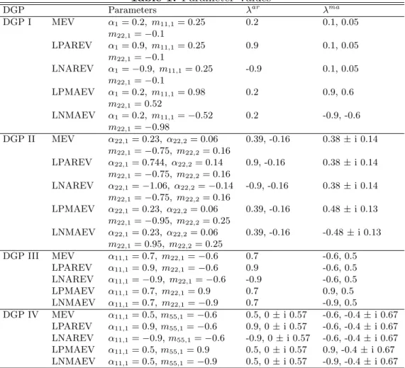
(30) 4.2 4.2.1. Generated Systems Small-Dimensional Systems. DGP I: The first two-dimensional process has been taken from Kapetanios (2003). This is a simple bivariate system in final equations form and was used in Kapetanios’s (2003) paper to demonstrate the virtues of the IOLS procedure. Precisely, the process is given by  α1 yt =  0.   0 m11,1 −0.20  yt−1 + ut +   ut−1 0.15 m22,1 α1 . and   1  Σ= . 0 1 This is an admittedly very simple process that is supposed to give an advantage to the IOLS procedure and also serves as a best case scenario for the VARMA algorithms because of its simplicity. The autoregressive polynomial has one eigenvalue and the moving-average polynomial has two distinct eigenvalues different from zero. Denote the eigenvalues of the autoregressive and moving-average part by λar and λma , respectively. These eigenvalues are varied and the remaining parameters, α1 , m11,1 and m22,1 are set accordingly. For this and the following DGPs, I consider parameterizations with medium eigenvalues (M EV ), large positive autoregressive eigenvalues (LP AREV ), large negative autoregressive eigenvalues (LN AREV ), large positive moving-average eigenvalues (LP M AEV ) and large negative moving-average eigenvalues (LN M AEV ). The parameter values corresponding to the different parameterizations can be found in table 1 for all DGPs. For the present process the M EV parametrization corresponds to the original process used in Kapetanios’s (2003) paper, with α1 = 0.2, m11,1 = 0.25 and m22,1 = −0.10. I fit restricted VARMA models in final equations form to the data. This gives a slight advantage to algorithms based on the VARMA formulation since in this case the CCA method has to 26.

(31) estimated relatively more parameters. For the CCA method the dimension of the state vector is set to the true McMillian degree which is two. DGP II: The second DGP is based on an empirical example taken from Lütkepohl (2005). A VARMA(2,2) model is fitted to West-German income and consumption data. The variables were the first differences of log income, y1 , and log consumption, y2 . More specifically, a VARMA (2,2) model with Kronecker indices (p1 , p2 ) = (0, 2) was assumed such that. yt.     0  0  0 0 =   yt−1 +   yt−2 + ut 0 α22,2 0 α22,1     0  0   0  0 +  ut−1 +   ut−2 0.31 m22,1 0.14 m22,2. and . . 1.44  −4 Σ=  × 10 . 0.57 0.82 While the autoregressive part has two distinct, real roots, the moving-average polynomial has two complex conjugate roots in the original specification. We vary again some of the parameters in order to obtain different eigenvalues. In particular, we maintain the property that the process has two complex moving-average eigenvalues which are less than one in modulus. The M EV parametrization corresponds to the estimated process with α22,1 = 0.23, α22,2 = 0.06, m22,1 = −0.75 and m̂22,2 = 0.16. These values imply the following eigenar ma = 0.375 + 0.139i, λma = 0.375 − 0.139i. Restricted values λar 1 = 0.385 λ2 = −0.159, λ1 2. VARMA models with restrictions given by the Kronecker indices were used. 4.2.2. Higher-Dimensional Systems. DGP III: I consider a three-dimensional system that was used extensively in the literature by, e.g., Koreisha & Pukkila (1989), Flores de Frutos & Serrano (2002) and others for illus27.

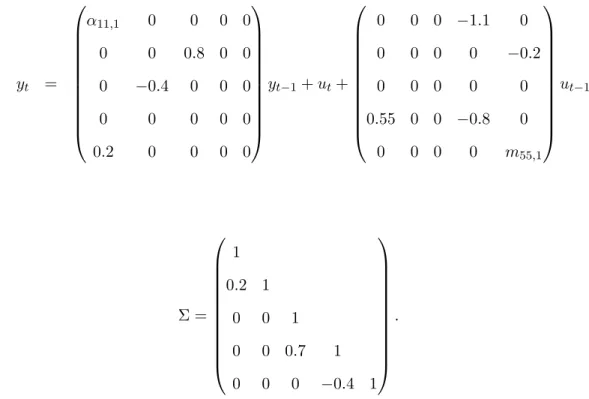
(32) trative purposes. Koreisha & Pukkila (1989) argue that the chosen model is typical for real data applications in that the density of nonzero elements is low, the variation in magnitude of parameter values is broad and feedback mechanisms are complex. The data is generated according to     0 0 1.1 α11,1 0 0       yt =  0 0  yt−1 + ut + 0 m22,1 0  ut−1  0     0 0 0.5 0 0.4 0 and . .  1     Σ = −0.7 1  .   0.4 0 1 The Kronecker indices are given by (p1 , p2 , p3 ) = (1, 1, 1) and corresponding VARMA models are fit to the data. While this DGP is of higher dimension, the associated parameter matrices are more sparse. This property is reflected in the fact that the autoregressive polynomial and the moving-average polynomial have both only one root different from zero. The parameters α11,1 and m22,1 are varied in order to generate particular eigenvalues of the autoregressive and moving-average polynomials as in the foregoing examples. The M EV specification corresponds to the process used in Koreisha & Pukkila (1989) and has ma eigenvalues λar = 0.7 and λma 1 = −0.6 and λ2 = 0.5.. DGP IV: This process has been used in the simulation studies of Koreisha & Pukkila (1987). The process is similar to the DGP III and is thought to typify many practical real data applications. In this study it is used in particular to investigate the performance of the algorithms for the case of high-dimensional systems. The five variables are generated. 28.

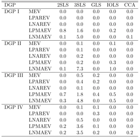
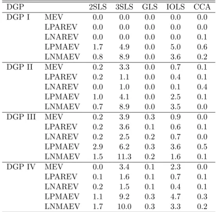
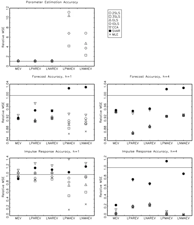
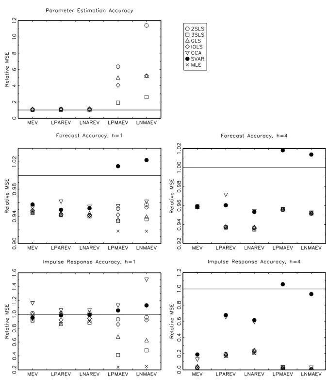
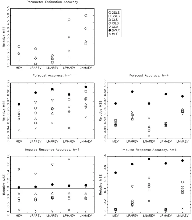
(33) according to the following VARMA (1,1) structure. yt.    0 α11,1 0 0 0 0        0  0 0 0.8 0 0        =  −0.4 0 0 0  yt−1 + ut +  0  0       0.55  0 0 0 0 0    0 0.2 0 0 0 0.  0 0 −1.1 0 0 0 0. 0.   0 0 −0.2    0 0 0   ut−1   0 −0.8 0   0 0 m55,1. and .  1.   0.2   Σ= 0   0  0.    1   . 0 1     0 0.7 1  0 0 −0.4 1. The true Kronecker indices are (p1 , p2 , p3 , p4 , p5 ) = (1, 1, 1, 1, 1) and corresponding VARMA models in Echelon form are fit to the data. The MEV parametrization corresponds to the one used by Koreisha & Pukkila (1987). That is, α11,1 = 0.5 and m55,1 = −0.6 with eigenvalues ar ma ma λar 1 = 0.5, λ2 = 0 ± i0.57, λ1 = −0.6 and λ2 = −0.4 ± i0.67.. 4.3. Results. The results are summarized in tables 2 to 5 and figures 1 to 8. The tables show the frequency of cases when the algorithms failed for different reasons. The figures plot the various MSE ratios discussed above. In the tables and figures, 2SLS, 3SLS and GLS are the two-stage, three-stage and generalized least squares methods, respectively, IOLS is the iterative least squares algorithm, CCA denotes the CCA subspace algorithm, SVAR is the VAR chosen by AIC and MLE is the maximum likelihood algorithm. Table 2 and table 3 display the frequency of cases when the algorithms yielded models that were not invertible or, in the case of the CCA algorithm, violated the minimum phase assumption for sample sizes T = 100 and T = 200, respectively. Apart from these cases, 29.

(34) there are also cases when the IOLS algorithm did not converge. The IOLS algorithm is regarded as non-convergent if it did not converge after 500 iterations. Furthermore, there are some very rare instances when the GLS algorithm returned estimated models that were extremely far from the true process (0.8 % in DGP III, LNMAEV, T=200). The tables 4 and 5 show the frequency of cases when the algorithms failed for one of the mentioned reasons in order to give a comprehensive picture of the reliability of the algorithms. First, as expected, the algorithms yield non-invertible models more frequently when the eigenvalues of the moving-average polynomial are close to one in absolute value, in particular in the case of large negative eigenvalues. Furthermore, as the number of estimated parameters increases, the algorithms yield non-invertible models more often. For 200 observations all algorithms become much more reliable in the sense that the number of estimated non-invertible models is much reduced. The most reliable algorithms are 2SLS, GLS and CCA. In particular, GLS and CCA yield non-invertible models for all algorithms and sample sizes in less than 1% of the replications. The 3SLS and the IOLS algorithm are the less reliable algorithms, although the IOLS algorithm can be quite stable. For particular DGPs, 3SLS can occasionally yield non-invertible models in more than 10 % of the cases. For some DGPs the IOLS algorithm does not converge relative frequently, but the problem becomes much less severe when the number of observations is increased to T = 200 as can be seen from tables 4 and 5. With respect to parameter estimation accuracy, the differences between the algorithms are generally more pronounced when the moving-average polynomial has eigenvalues that are close to one in absolute value. The differences become also more pronounced when the number of observations increases but the ranking of the algorithms remains unchanged, in general. The 2SLS algorithm is dominated by the other algorithms, aside from one case (DGP III, LNMAEV). The parameter estimation accuracy of the GLS estimator is much better but close to the accuracy of the 2SLS algorithm for higher-order processes, although in cases with large negative moving-average eigenvalues the estimator might be relatively accurate. The IOLS estimator is in most cases much better than 2SLS and its advantage becomes most pronounced in the high-dimensional case IV. Compared to the GLS algorithm, IOLS can be worse for small-dimensional systems but the ranking changes for the higher. 30.

(35) dimensional processes. The 3SLS estimator is always superior to any other method, apart from MLE. In particular, the 3SLS method is much better when the number of estimated parameters increases, that is for DGP III and IV. However, the MLE method is in this context much more accurate and is often twice as good as the 3SLS method. Summarizing, the 3SLS procedure is the best alternative to MLE despite the high number of cases when the algorithm yielded non-invertible model. Nevertheless, even the best alternative can be quite imprecise compared to MLE. This does not necessarily mean that 3SLS is not a relatively good estimator because the MLE procedure starts with the true parameter values and therefore the procedure represents an ideal case in this context. The differences in terms of forecasting precision are less pronounced. Additionally, even though some algorithms do estimate the parameters more accurately than others, they are not necessarily superior in terms of forecasting accuracy. The ranking might change. Not surprisingly, in almost all cases the VARMA algorithms do better than the benchmark long VAR. In most cases, the VARMA algorithms also display smaller MSE ratios than a VAR chosen by AIC. However, given that the orders of the VARMA models are fixed and correspond to the true orders, the comparison is biased in favor of VARMA modelling. Increasing the forecast horizon, does reduce the differences between the different algorithms. The same is true when more observations are available. Increasing the complexity in terms of Kronecker indices does have minor effects. The forecasts obtained by the CCA method are often comparable but often also inferior to the forecasts obtained by other algorithms. In particular, the CCA forecasts are often inferior for the one-step forecast horizons. The 2SLS estimator yields usually better forecasts than the CCA forecasts and comparable but sometimes slightly worse forecast than the other VARMA algorithms. The GLS and the IOLS procedure do quite well in forecasting depending on the specific DGP and number of observations. The 3SLS procedure, however, seems to be slightly preferable. The MLE method is always superior to all simple algorithms apart from one case, DGP III, LNMAEV with T = 100, where its MSE is roughly three times as large as the MSE of the other VARMA algorithms. In this case, the MSE ratio for the MLE procedure is not shown on the graph since this would imply loosing important details in other parts. In general, however, the differences are small, in particular in comparison to. 31.

(36) the rather large differences in terms of parameter estimation accuracy. In sum, the ranking of the different algorithms becomes less clear when forecasting is the objective. While the VARMA methods do generally better than the VARs and the CCA method, the differences are often small. For the simulated processes, 3SLS is a good alternative algorithm to MLE if forecasting is the objective. The precision of the estimated impulse responses varies much more between the algorithms. In most cases the VARMA algorithms do comparably or better than the VAR approximations but, as mentioned above, this comparison is biased in favor of VARMA modelling. When the impulse response horizon is increased, VARMA modelling becomes much more advantageous in comparison with the VAR approximations. At short horizons the picture is rather mixed depending on the algorithms and DGPs. For example, for the rather simple DGP I, there are little advantages of VARMA modelling apart from the LPMAEV and LNMAEV parameterizations. For the other DGPs there are in principle considerable advantages provided that the right algorithm is chosen and the process is correctly specified. Furthermore, the VARMA algorithms differ much more at horizon h = 1. Increasing the sample size has no important effect on the ranking of the algorithms. First, the CCA method seems to be inferior to the VARMA algorithms for all DGPs and both horizons. Occasionally, CCA is worse than the VAR chosen by AIC. The 2SLS algorithm estimates the impulse responses with comparable or slightly worse accuracy than the other VARMA algorithms. Only for DGP II the impulse response estimates obtained by 2SLS are as precise as the estimates obtained by other algorithms. Also the results for the impulse response estimates obtained by GLS are mixed. In some cases, such as DGP I with large moving-average eigenvalues, GLS is performing quite well but in most other cases GLS is inferior to IOLS or 3SLS. In fact, these two algorithms estimate the impulse response function best in most of the cases. While the performance of IOLS in this respect depends still on the specific DGP, 3SLS is almost always the preferable method. Furthermore, even though IOLS is often the second-best method, the difference to 3SLS can be considerable, in particular for higher-order processes. In sum, the 3SLS procedure is by far preferable, independent of the specific DGP at hand. Generally, the impulse response estimates obtained by MLE are much more precise than the corresponding. 32.

(37) estimates obtained by the 3SLS algorithm. These results correspond to the statements made above about the algorithms’ relation in terms of parameter estimation accuracy. Overall, VARMA modelling turns out to be potentially quite advantageous if one is interested in the impulse responses of the DGP. The precision obtained by MLE is, however, rarely obtained by any of the simpler VARMA estimation algorithms. In sum, VARMA modelling can be advantageous. While the advantages are potentially minor with respect to forecasting precision, the results suggest that the impulse responses can be estimated more accurately by using VARMA models, provided that the model is specified correctly. Apart from forecasting, there are large differences between the algorithms. Overall, the algorithm, which is closest to maximum likelihood estimation, 3SLS, seems to be superior to any other of the simpler estimation algorithms. In particular, when the complexity of the simulated systems increases, 3SLS is the only algorithm that almost always outperforms the benchmark VARs in terms of accuracy of the estimated impulse responses. A concern, however is the instability of the algorithm in the presence of large eigenvalues of the moving-average polynomial. Even though full-information maximum likelihood would be the ideal algorithm, 3SLS is performing quite well in comparison not only to the alternative simple VARMA algorithms but also in comparison to the benchmark VARs. However, as the algorithm is implemented here, it is still not stable enough in order to be used in a automatic fashion because of the non-invertibility problem. Given the simplicity of the used DGPs and that complications such as specification, outliers etc. are neglected, these results suggest that the 3SLS algorithm would have to be improved considerably in order to create an algorithm that returns accurate estimates in almost all cases.. 5. Conclusion. Despite the theoretical advantages of VARMA models compared to simpler VAR models, they are rarely used in applied macroeconomic work. While Gaussian maximum likelihood estimation is theoretically attractive, it is plagued with various numerical problems. Therefore, simpler estimation algorithms are compared in this paper by means of a Monte Carlo. 33.

(38) study. The evaluation criteria used are the precision of the parameter estimates, the accuracy of point forecasts and the accuracy of the estimated impulse responses. The VARMA algorithms are also compared to two benchmark VARs in order to judge the potential merits of VARMA modelling. It has been shown in the simulations that there are situations where the investigated algorithms do not perform very well. There is a rough trade-off between the technical reliability of the algorithms and the quality of the estimates. With respect to the accuracy of the parameter estimates, the iterative least squares procedure of Kapetanios (2003) and the simple least squares procedure of Hannan & Kavalieris (1984a) seem to perform relatively well for smaller processes with small eigenvalues of the moving-average part. However, they can be quite imprecise relative to exact maximum likelihood for higher dimensional processes and in particular for processes with large eigenvalues in the moving-average part. If the purpose of time series analysis is forecasting, the methods perform approximately comparable though few can reach or outperform the forecasting power of exact maximum likelihood. The gains from using VARMA models in contrast to VARs appear to be relatively small. Also, in this case the procedure of Hannan & Kavalieris (1984a) turned out to be preferable over the other simpler estimation algorithms. The true impulse responses are estimated poorly by most algorithms given the benchmark of a long VAR. Again, the procedure of Hannan & Kavalieris (1984a) is potentially quite advantageous. Also the iterative least squares procedure of Kapetanios (2003) is performing well in this respect. Nevertheless, the algorithms cannot reach the precision of the exact maximum likelihood procedure. It turns out, that the only simple procedure that reliably gave significantly better results than the benchmark VARs in terms of the accuracy of the derived forecasts and impulse response estimates, is the procedure which is closest to maximum likelihood, namely the procedure of Hannan & Kavalieris (1984a). However, this procedure is also the most unreliable procedure in technical terms, in that it often yields estimated models which are not invertible. Given the simplicity of the simulated data generating processes, the algorithm would have to be improved considerably in order to make it a standard tool for applied researchers.. 34.

(39) A reliable and accurate algorithm for the estimation of VARMA models still remains to be developed. This study suggests that there are potentially considerable gains from VARMA modelling. Such an algorithm would have to be able to deal with various issues which are not considered in this study. The algorithm should work well in the case of integrated and cointegrated multivariate series. The algorithm must give reasonable results with extremely over-specified processes as well as in the presence of various data irregularities such as outliers, structural breaks etc. The applicability of such an algorithm would also crucially depend on the existence of a reliable specification procedure. These topics, however, are left for future research.. 35.

(40) References Akaike, H. (1974), ‘A new look at the statistical model identification’, IEEE Trans. Autom. Control AC-19 pp. 716–723. Aoki, M. (1989), State Space Modeling of Time Series, Springer-Verlag, Berlin. Bauer, D. (2005a), ‘Comparing the CCA subspace method to pseudo maximum likelihood methods in the case of no exogenous inputs.’, Journal of Time Series Anaysis 26(5), 631– 668. Bauer, D. (2005b), ‘Estimating linear dynamical systems using subspace methods’, Econometric Theory 21, 181–211. Cooley, T. F. & Dwyer, M. (1998), ‘Business cycle analysis without much theory. A look at structural VARs’, Journal of Econometrics 83, 57–88. Deistler, M., Peternell, K. & Scherrer, W. (1995), ‘Consistency and relative efficiency of subspace methods’, Automatica 31, 1865–1875. Desai, U. B., Pal, D. & Kirkpatrick, R. D. (1985), ‘A realization approach to stochastic model reduction’, International Journal of Control 42(4), 821–838. Dufour, J.-M. & Pelletier, D. (2004), ‘Linear estimation of weak VARMA models with a macroeconomic application’. Université de Montréal and North Carolina State University, Working Paper. Durbin, J. (1960), ‘The fitting of time-series models’, Revue de l’Institut International de Statistique / Review of the International Statistical Institute 28(3), 233–244. Fernández-Villaverde, J., Rubio-Ramı́rez, J. & Sargent, T. J. (2005), ‘A,B,C’s (and D)’s for understanding VARs’. NBER Technical Working Paper 308, May draft. Flores de Frutos, R. & Serrano, G. R. (2002), ‘A Generalized Least Squares Estimation Method For VARMA Models’, Statistics 13(4), 303–316.. 36.

(41) Hannan, E. J. & Deistler, M. (1988), The Statistical Theory of Linear Systems, Wiley, New York. Hannan, E. J. & Kavalieris, L. (1984a), ‘A method for autoregressive-moving average estimation’, Biometrika 71(2), 273–280. Hannan, E. J. & Kavalieris, L. (1984b), ‘Multivariate linear time series models’, Advances in Applied Probability 16(3), 492–561. Hillmer, S. C. & Tiao, G. C. (1979), ‘Likelihood function of stationary multiple autoregressive moving average models’, Journal of the American Statistical Association 74, 652–660. Kapetanios, G. (2003), ‘A note on the iterative least-squares estimation method for ARMA and VARMA models’, Economics Letters 79(3), 305–312. Kavalieris, L., Hannan, E. J. & Salau, M. (2003), ‘Generalized Least Squares Estimation of ARMA Models’, Journal of Time Series Anaysis 24(2), 165–172. Koreisha, S. & Pukkila, T. (1987), ‘Identification of Nonzero Elements in the Polynomial Matrices of Mixed VARMA Processes’, Journal of the Royal Statistical Society. Series B 49(1), 112–126. Koreisha, S. & Pukkila, T. (1989), ‘Fast Linear Estimation Methods for Vector ARMA Models’, Journal of Time Series Anaysis 10(4), 325–339. Koreisha, S. & Pukkila, T. (1990), ‘A generalized least squares approach for estimation of autoregressive moving average models’, Journal of Time Series Analysis 11(2), 139–151. Koreisha, S. & Pukkila, T. (1990a), ‘Linear methods for estimating ARMA and regression models with serial correlation.’, Communications in Statistics-Simulation 19, 71–102. Larimore, W. E. (1983), System Identification, Reduced-Order Filters and Modeling via Canonical Variate Analysis, in H. S. Rao & P. Dorato, eds, ‘Proc. 1983 Amer. Control Conference 2’.. 37.

(42) Lütkepohl, H. (2005), New Introduction to Multiple Time Series Analysis, Springer-Verlag, Berlin. Lütkepohl, H. & Poskitt, D. S. (1996), ‘Specification of Echelon-Form VARMA Models’, Journal of Business & Economic Statistics 14(1), 69–79. Mauricio, J. A. (1995), ‘Exact maximum likelihood estimation of stationary vector ARMA models’, Journal of the American Statistical Association 90(429), 282–291. Newbold, P. & Granger, C. W. J. (1974), ‘Experiences with forecasting univariate time series and combination of forecasts’, Journal of the Royal Statistical Society A137, 131–146. Poskitt, D. S. (1992), ‘Identification of echelon canonical forms for vector linear processes using least squares’, Annals of Statistics 20, 196–215. Reinsel, G. C. (1993), Elements of Multivariate Time Series Analysis, Springer-Verlag, New York. Van Overschee, P. & DeMoor, B. (1994), ‘N4sid: Subspace algorithms for the identification of combined deterministic-stochastic processes’, Automatica 30(1), 75–93.. 38.

(43) A. Equivalence between VARMA and State Space Representations. This discussion serves as an illustration and is based on the corresponding sections in Aoki’s (1989) book.7 It is not claimed, for example, that the following state space representation of a VARMA model is especially meaningful. The point is simply to demonstrate that a VARMA model can be written in state space form. Suppose that a multiple time series yt = (y1t , . . . , yKt )0 of dimension K satisfies a VARMA(p, q) model given by yt =. p X. Ai yt−i + ut +. i=1. q X. Mi ut−i ,. i=1. where A0 = IK is assumed for simplicity. This process can be written as a state space model by defining             A :=           .  A1 . . . . . . Ap M1 M2 . . . Mq    0 0 IK 0    .. .. .. . . .  0    IK 0   , ((p + q)K × (p + q)K),  0 0 0    ..  . 0 IK 0   .. ..  . .   0 IK 0. · B. 0. :=. ¸. C :=. , (K(p + q) × K), ¸ : M1 : . . . : Mq , (K × K(p + q)).. IK : 0 : . . . IK : . . . : 0 · A1 : . . . : Ap. 7. See also the book of Hannan & Deistler (1988) for an extensive discussion on the relation between state space and VARMA models.. 39.

(44) The state space model is of the form. xt+1 = Axt + But , yt = Cxt + ut , with a state vector given by . xt.  yt−1  .  ..     yt−p =    ut−1   .  ..   ut−q.          , ((p + q)K × 1).       . Given a state space model of order n for a K-dimensional process, let the characteristic polynomial of the system matrix A be |A − λIn | = c0 λn + c1 λn−1 + c2 λn−2 + . . . + cn , c0 = 1. Multiply the observation equation for t, . . . , t + n with the coefficients ci , i = 0, . . . , n, in the following way. cn yt = cn (Cxt + ut ), cn−1 yt+1 = cn−1 (CAxt + CBut + ut+1 ), .. . yt+n = CAn xt + CAn−1 But + . . . + CBut+n−1 + ut+n , where the right hand side has been obtained by recursive substitution. Summing up these equations one obtains n. n−1. yt+n + c1 yt+n−1 + . . . + cn yt = C(A + c1 A. + . . . + cn In )xt +. n X i=0. 40. Di ut+i.

(45) where Di = cn−i IK +. Pn−i. k=1 cn−i−k CA. k−1 B.. According to the Cayley - Hamilton theorem,. the matrix polynomial in A vanishes, An + c1 An−1 + . . . + cn In = 0 (Aoki 1989). One obtains therefore the following VARMA representation. yt+n + c1 yt+n−1 + . . . + cn yt =. n X i=0. 41. Di ut+i ..

No results found