VENTILATION CALCULATION BY NETWORK MODEL
INDUCING BI-DIRECTIONAL FLOWS IN OPENINGS
Katsumichi Nitta
Department of Architecture and Design,
Faculty of Engineering and Design,
Kyoto Institute of Technology.
Kyoto, P.O.Box 606-8585, Japan.
ABSTRACT
For the multi-room ventilation calculations, bi- directional flows or counter flows in openings have been rarely taken into consideration and only uni-directional flows have been allowed for the calculation. It stands to reason that the calculation requires quite sophisticated scheme and the appearance of the bi-directional flows are restricted only to a limited number of openings neighboring the neutral plane of the building and also the flow rates may be too little to affect the total building ventilation.
The existence of the bi-directional flows, however, is significant as it may promote the heat exchange between the adjacent rooms and affect the problem in the fire safety or the generation of the ventilation variety.
In this paper, the modified ventilation calculation method using the network model is proposed, in which the effect of the bi-directional flows is partially included without the inordinate expansion of the computer capacity. The examination of the existence of the bi-directional flows, the errors in flow rates and the difference of the ventilation modes are investigated with the ordinary and modified ventilation calculations for the stairwell attached two- and three- story houses.
INTRODUCTION
Recently the natural ventilation, especially the buoyancy or stack ventilation, has been introduced in the building from the viewpoint of the saving of energy or the environmental symbiosis. For the prediction of multi- story building ventilations, the CFD (Computer Fluid Dynamics) analyses are not yet available gears both in hardware and software and the multi-room ventilation calculation by the network model based on the lumped constant circuits have been still in use.
In this paper, the fundamental equations based on the network model restricted to uni-directional opening flows and the modified network model which permits bi-directional flows are shown in the first place. All of the known variables such as flow rates, temperatures and pressure differences are treated as vectors, and the incidence matrix and loop matrix are introduced for the matrix operation. As the related equations are non-linear, the successive numerical calculation by Newton- Raphson method is adopted and the Kirchhoff’ second law is used for the ventilation circuits by reasons of the
stable convergence and the reduction of unknown variables related to the capacity of the computer.
In the network model all of the adjacent rooms (or nodes) do not have to be connected with the bi-directional flows (or couple of blanches) and only the small number of openings near half the height of the building should be checked for the bi-directional flows. The modified network model allowed for these bi-directional flows is proposed. This model starts from the converged result by the ordinary network model. From the vertical pressure difference distributions in openings, potential openings of bi-directional flows are picked up and the circulations which compensate the flow rate difference by the counter flow in such opening are added to the thermal balance equation, and the successive calculation is continued to the convergence.
Errors in both flow rates and heat calorie caused by the hypothetical type of the pressure distributions which is uniform, gradient and involving the neutral plane are estimated. And the effect of the bi-directional flows in openings on the ventilation rates and modes (or flow directions) are investigated using the models of the stairwell attached two- and three story houses.
VENTILATION CALCULATION BY
NETWORK MODEL
The outline of the calculation of the multi-room ventilation based on the ordinary network model is introduced. The electric analogous circuit is the fundamental concept and so a node corresponds to a uniform room temperature and a branch corresponds to an opening. Kirchhoff’ first and second laws can be applicable but the latter is used in this paper for the sake of the stable convergence of the solutions.
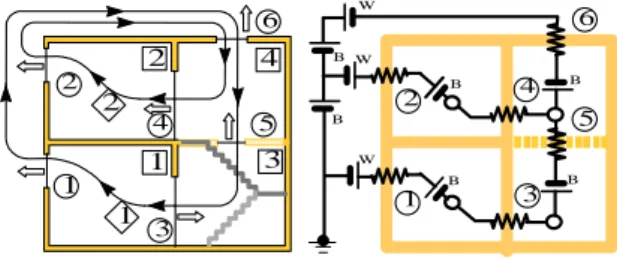
Ventilation Network Model
The model is illustrated in Fig. 1(A). Temperature in the room is assumed to be uniform and the flow resistances occur only in the openings. The pressure difference distribution before and after an opening is supposed to be uniform and it take the value of middle height and so only the uni-directional flows are supposed . We name such the opening an orifice.
The ventilation network is constructed as shown in Fig. 1(B) by representing a room temperature as a node
Eighth International IBPSA Conference Eindhoven, Netherlands August 11-14, 2003
G G (A) (B) divergence convergence Repetition Overflow ) 2 ( ] 0 [ ] ][ [ T = L I
[ ]
[ ]
Loops Rooms L I Openings Openings ) 1 ( 1 0 1 0 1 0 1 1 0 1 0 1 2 1 , 1 1 1 0 0 0 0 1 0 1 0 0 0 0 1 0 1 0 0 0 0 1 0 1 4 3 2 1 6 5 4 3 2 1 6 5 4 3 2 1 »¼ º «¬ ª − + + − − − + = » » » ¼ º « « « ¬ ª + − + + − − + + + ={ }
(3) ˆ ˆ ˆ , } { 0 0 0 0 0 0 °¿ ° ¾ ½ °¯ ° ® + = °¿ ° ¾ ½ °¯ ° ® + = θ ρ ρ θ ρ ρ T T T Tand an opening is expressed as a branch. Temperature, flow characteristics of opening and buoyancy corresponds to electric potential, resistance and battery of an electric circuit respectively. If the room temperature does not designated, the buoyancy force ( or battery in Fig. 1) is also unknown. Out air temperature and the wind force are known variables.
Figure 1. Ventilation Network Model
Room Pressures Assumption Method and Loop Flow Rates Assumption Method
The ventilation calculation is usually executed by the successive numerical procedures since the flow characteristics which are the relation between the flow rate and the pressure loss in the opening and the equation of state which is the relation between the air temperature and the density are nonlinear.
There are two numerical calculation algorithms. One is the room pressures assumption method in which the room static pressures are principal unknown variables and Kirchhoff’s first law is adopted, and the other is the loop flow rates assumption method in which the flow rates of independent loops in the network are solved with Kirchhoff’s second law.
The good and bad points of two methods are compared. Here we prescribe for the building conditions that the number of the rooms, rooms of fixed heat supply (including zero) and openings, is M, K (
0
≤
K
≤
M
) and N respectively. So the number of the unknown variables to solve the ventilation problem is as follows.Room Pressures Method: R = M+K Loop Flow Rates Method: L = N-M
The ventilation shown in Fig. 1 is the perfect buoyancy ventilation assigned the numbers of M=4, K=4, N=6, and so R=8 and L=2.
Figure 2. Two Gradients used in Newton-Raphson Method
The unknown variables for the loop flow rates assumption method is commonly less than the other for common buildings. Furthermore, the loop flow rates assumption method have an advantage of a good convergence in the successive calculation. Usually the Newton-Raphson method is introduced for numerical calculation, and ∂G/∂(∆p) for the room pressures method and ∂(∆p)/∂G for the loop flow rates method is operated as shown in Fig. 2. If the flow rate G or the pressure difference ∆p through an opening might be very small on a certain stage of the calculation, the former method may have infinity in the gradient and the operation must be stopped, while the latter method must take zero gradient and there is no problem.
In this paper, we adopt the loop flow rates assumption method for the above reason. An example of the loops is illustrated in Fig. 1(A) but the other independent loops may be set, as the network has a kind of freedom in decision.
Fundamental Equations
Fundamental equations are expressed by the matrix form, and the successive numerical calculation may be done by the matrix operation. In the first place, the directions of the flows in openings and loops are arbitrary set in advance. Then the incidence matrix
[
I
]
and the loop matrix [L] which are used in the graph theory are introduced as shown in Eq. (1) by reference to Fig.1.Element ij of the incidence matrix
[
I
]
means the link of the i-th room with j th opening, and +1 and -1 represents the outflow and the inflow respectively according to the presetting direction as shown in Fig.1(A). Element Lij of the loop matrix [L] means the coincidence or not with the presetting loop flow direction. Here,[
I
]
always has the orthogonal relation with[
L
]
as shown in Eq. (2).Fundamental equations are as follows.
(i) State equations for air in the room and in the opening: The density is varied with temperature and so Boussinesq approximation is not applied. Temperatures in the openings {
θ
} may be admitted the negative number for convenience of the calculation of heat calorie (cf. Eq. (10)’).(ii) Flow rates relation ship between openings and loops: (B) B W B B B W W B B
B: Buoyancy, W: Wind Pressure
(A) 1 4 2 3 5 6 2 3 4 5 6 1 2 3 4 1 2 1 ) ( p G ∆ ∂ ∂ p ∆ p ∆ 0 ) ( 0 = ∂ ∆ ∂ = G G p ∞ = ∆ ∂ ∂ = ∆ 0 ) ( p p G G p ∂ ∆ ∂( )
{ }
~ (4) ] [ } {G = LT G) 5 ( } { 2 1 } { 2 d A G p ¸ ¹ · ¨ © § = ∆ α ρ
{ }
ˆ, { }[ ]
{ }
ˆ (10) ] [ } {θ = F θ ρ = F ρ{ }
[ ]
{ }
{ } { } { }
(13) ~ ~ ~ ~ ~ 1 1 1 ) ( 1 °¿ ° ¾ ½ ∆ + = ∆ − = ∆ + + − + j j j j j j G G G p Z G ) 15 ( ) 0 ( 2 ) ( ≥ ¿ ¾ ½ ¯ ® ∆ = ¿ ¾ ½ ¯ ® ∂ ∆ ∂ G p G p )' 6 ( 0 0 0 ˆ 0 0 0 0 0 0 0 0 0 0 0 0 0 0 0 0 0 0 0 0 0 0 0 0 0 0 0 0 0 0 1 1 1 0 0 00 1 0 10 01 0 1 00 00 1 0 00 1 1 6 5 4 3 2 1 6 5 4 3 2 1 ° ¿ ° ¾ ½ ° ¯ ° ® = ° ° ¿ ° ° ¾ ½ ° ° ¯ ° ° ® » » » » » » ¼ º « « « « « « ¬ ª » » » ¼ º « « « ¬ ª − − − W G G G G G G Cp θ θ θ θ θ θ °¿ ° ¾ ½ °¯ ° ® = ¸ ¸ ¸ ¸ ¸ ¸ ¹ · ¨ ¨ ¨ ¨ ¨ ¨ © § ° ¿ ° ¾ ½ ° ¯ ° ® − − − − » » » » » ¼ º « « « « « ¬ ª − − − » » » » » » ¼ º « « « « « « ¬ ª + ° ° ¿ ° ° ¾ ½ ° ° ¯ ° ° ® ∆ ∆ ∆ ∆ ∆ ∆ »¼ º «¬ ª − − − − 0 0 0 0 ˆ ˆ ˆ ˆ ˆ ˆ ˆ ˆ 1 0 0 0 1 1 0 0 1 0 1 0 0 1 0 1 0 0 1 0 0 0 0 1 0 0 0 0 0 0 0 0 0 0 0 0 0 0 0 0 0 0 0 0 0 0 0 0 0 0 0 0 0 0 0 1 0 1 0 1 0 1 1 0 1 0 1 0 4 0 3 0 2 0 1 5 4 3 2 1 6 5 4 3 2 1 g h h h h h p p p p p p ρ ρ ρ ρ ρ ρ ρ ρ[ ]
{ }
{ }
(10)' ˆ ˆ ˆ ˆ 0 0 ˆ ˆ ˆ ˆ 0 0 ; 1 0 0 0 0 1 1 0 1 0 1 01 0 1 0 1 1 1 01 0 0 0 4 3 2 1 4 3 2 1 ° ° ¿ ° ° ¾ ½ ° ° ¯ ° ° ® = ° ° ° ¿ °° ° ¾ ½ ° ° ° ¯ °° ° ® = » » » » » ¼ º « « « « « ¬ ª − − − = ρ ρ ρ ρ ρ θ θ θ θ θ and F(iii) Opening characteristics (corresponding to the momentum equation):
where,
G
∝
∆
p
is admitted for all openings. The flow rate G gets the positive sign when the flow dirction coincides with the initial setting one as shown in Fig.1 and the negative sign for the reverse flow. The pressure drop∆pis set the same sign with G, namely G⋅∆p≥0 .(iv) Heat balance equation:
This equation is applied to the room setting of heat supply rate and so it is not used for the room of fixed temperature. The component Uij(i≠ j) is the heat conductance of the wall between i-th and j-th room and
here, Uiois the heat conductance of the building enclosure. If i-th and j-th rooms are next door to each other, Uij= 0. For the example in this paper, all of the walls are insulated and so [U]=[0] and the heat is supplied only to the room on the first floor.
(v) Flow rate balance equation ( Node equation): By Kirchhoff’s first law,
If the flow rates assumption method is adopted, this equation is indispensable. But if the loop flow rates assumption method is used, this equation is inevitably satisfied, inducing from Eqs. (2) and (4).
(vi) Pressure balance equation ( Circuit equation): By Kirchhoff’s second law, the sum of pressure losses along the every closed loop as shown in Fig. 1 must be
zero and so,
In our example, the windless condition {pW}={0} is set and the concrete equation is as follows.
(9)’ (vii) Estimation of temperatures and densities through the openings from the variables in the rooms:
The flow direction in any opening is usually unknown but it is indispensable for calculation of heat balance or pressure loss in flow loops. In this paper the iterative method is introduced.
where, the transformation matrix [F] is defined by
Here the operator FIX rounds the decimals down to integers and {d} is the flow direction vector decided in the last step of successive calculation.
If the flow directions of 3rd, 4th and 5th opening are coincident with the preset ones and the other directions are opposite, for the next step
For the instance previously used,
Successive Numerical Calculation
The set of the ventilation equations should be solved numerically as this system is non-linear judging from Eqs. (6) and (8). We execute the ventilation calculation by Newton-Raphson iteration method based on the loop flow rates assumption technique.
If the room pressure assumption method is adopted, the residual error in Eq. (8) must be converged to zero and if the loop flow rate assumption method used in this paper is introduced, the residual error in Eq. (9) must be dissolved.
Supposing that the loop pressure losses
{ }
∆
p
~
jwere caused in the left side of Eq.(9) after the j-th stage of the calculation, the setting values of the loop flow rates{ }
~ j+1G at the next (j+1)th stage might be given as follows.
where, [Z] is a revision matrix in the Newton- Raphson method. When all the rooms are set by the heat supply like in our example, [Z] is get as shown in Eq.(14). If a part of the rooms are set by the temperature or the prescribed forced ventilation by fan is used, the representation of [Z]comes to be very sophisticate. See the reference (Nitta, 1994).
where, the pressure gradients are calculated from Eq. (8) as follows.
MODIFIED NETWORK MODEL FOR
BI-DIRECTIONAL FLOWS IN OPENINGS
For the ordinary ventilation network, only the uni-directional flow (or orifice flow) is supposed in one opening. If the floors of multi-story building are numerous, the neutral plane of the pressure appears near the middle height of the building and the bi-directional
{ } { }
ˆ ˆ (6) ] [ } { ] [I G U W Cp θ − θ = ) 7 ( , 0¦
≠ = − = M i j j ij ii U U ) 8 ( } 0 { } ]{ [I G ={
} { }
(
{ } [ ] ˆ ˆ)
{0} (9) ] [ ∆ + − 0 − W = T p g I h p Lρ
ρ
) 11 ( } 1 }{ { ] ([ 2 1 ] [ » ¼ º « ¬ ª ¸ ¹ · ¨ © § + = T T d I FIX F ) 12 ( } , , , , ( } {d d1 d2 d3 d4 d5 T = )' 12 ( } 1 , 1 , 1 , 1 , 1 , 1 { } { T = − − + − + + d[ ]
() [ ] ( ) [ ]T (14) j j L G p L Z ∂ ∆ ∂ =) 17 ( ) 0 ( 1 ) 0 ( 0 ) 0 ( 1 ) ( °¯ ° ® < − = > + = x x x x sign ) 18 ( ˆ ˆ , ) ( j0 j k i j z p gz p =∆ +∆ρ ∆ρ=ρ −ρ ∆ ) 19 ( 0 g p h j j nj ∆ρ ∆ − = ) 20 ( jC jH j G G G = + ) 21 ( 2 3 * 2 3 * 2 2 3 2 ) ( 2 2 3 2 ) ( ° ° ° ¿ °° ° ¾ ½ ¸¸¹ · ¨¨© § + ∆ ∆ − = ¸¸¹ · ¨¨© § − ∆ ∆ = nj j j jD j j jD nj j j jH j j jH h H g B sign G h H g B sign G ρ ρ α ρ ρ ρ α ρ
{
}
{
ˆ ˆ}
( )( ) (22) 2 1 ) )( ( ˆ ˆ 2 1 ° ¿ ° ¾ ½ − ∆ − + = − ∆ + + = jd ju j k i jC jd ju j k i jH sign sign ρ ρ ρ ρ ρ ρ ρ ρ ρ ρ ρ ρ ) 23 ( jC jH j G G G ≠ + ) 25 ( ) 1 ( 1 1 , 1 =− − ≠ − = G r r G G r r GjH j jC j ) 26 ( 2 1 1 3 / 1 3 / 1 j jH jC jH jC j n H h ⋅ ¸ ¸ ¹ · ¨ ¨ © § + ¸ ¸ ¹ · ¨ ¨ © § − = ρ ρ ρ ρ ) 27 )( 1 ( 2 2 3 2 ) ( 2 / 3 = ¸¸¹ · ¨¨© § − ∆ ∆ = − = G sign B g H h r G nj j j jH j j jC jH ρ α ρ ρ(
,)
( 0) (28) min ~ = > jC jH ik B G G G[
]
{ } { }
ˆ ˆ (29) } { ] [I G U C G W Cp θ − + p B θ = ) 30 ( , 0¦
≠ = − = M i j j ij B ii B G G ) 24 ( ) 0 ( 2 / 2 / 3 > ¸ ¸ ¹ · ¨ ¨ © § + − ¸ ¸ ¹ · ¨ ¨ © § = − = nj j nj j jC jH jC jH h H h H G G r ρ ρflows may be restricted to several openings. As these flows are accompanied by the heat exchange between rooms, the ventilation mode (namely the pattern of the flow directions and flow rates) may vary from the case of uni-directional flows only.
However the number of the openings in which the neutral planes are involved must be very small in comparison with the total number of the whole openings in a building. Allocation of the bi-directional branches for all openings is too complicate to be realistic by reason of the increase of not only the number of branches but also the additive information about the another unknown neutral plane heights.
Calculation Procedures
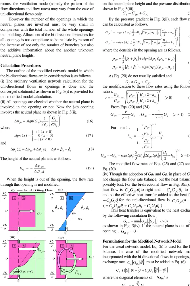
The outline of the modified network model in which the bi-directional flows are in consideration is as follows. (i) The ordinary ventilation network calculation for the uni-directional flows in openings is done and the converged solution(s) as shown in Fig. 3(i) is provided for this modified model calculation.
(ii) All openings are checked whether the neutral plane is involved in the opening or not. Now the j-th opening involves the neutral plane as shown in Fig. 3(ii).
where
and
The height of the neutral plane is as follows.
When the height is out of the opening, the flow rate through this opening is not modified.
Figure 3. Modification concept of bi-directional flow
(iii) Rates of inflow GjC and outflow GjH in such opening
of the potentially bi-directional flow are calculated based on the neutral plane height and the pressure distribution as shown in Fig. 3(iii).
By the pressure gradient in Fig. 3(ii), each flow rates can be calculated as follows.
where the densities in the opening are as follows.
As Eq. (20) do not usually satisfied and
the modificastion to these flow rates using the following ratio r.
From Eqs. (20) and (24),
For r = 1 ,
The modified flow rates of Eqs. (25) and (27) satisfy Eq. (20).
(iv) Though the adoption of GjHand GjCin place of Gjdo not change the flow rate balance, but the heat balance is possibly lost. For the bi-directional flow in Fig. 3(iii), the heat flow is
C
pG
jHθ
ito right and−
C
pG
jCθ
k to left, and so the effective heat transfer added to the heat flowi j pG
C
θ
− for the uni-directional flow is CpGjC(θi−θk)
) (=CpGjHθi+CpGjCθk −CpGjθi .
This heat transfer is equivalent to the heat exchange by the following circulation flow
as shown in Fig. 3(iv). If the neutral plane is out of the opening j, G~Bsj=0.
Formulation for the Modified Network Model
For the usual network model, Eq. (6) is used for the heat balance. In case of the modified network model incorporated with the bi-directional flows in openings, the exchange rate
[ ]
{ }
θˆB p G
C must be added in Eq. (6).
where the diagonal elements of [GB] is
) 16 ( 2 1 ) ( 2 0 ¸¸ ¹ · ¨ ¨ © § = ∆ j j j j j A G G sign p α ρ 0 Hj 2 -Hj 2 0 Hj 2 -Hj 2 0 Hj 2 -Hj 2 0 Hj 2 -Hj 2 ; ; ; ; Gj hnj pj0 GjH GjC(<0) Gj (i) (ii) (iii) (iv)
Initial Setting Flow
i k i k i k i k i i ρ θˆ, ˆ ik B G~ ik B G~ k k ρ θˆ,ˆ
) 31 ( ) (z p0 gz pj =∆ j +∆ρj ∆
(
) (
)
¿ ¾ ½ ¯ ® ∆ +∆ −∆ −∆ ∆ = 2 3 0 2 3 0 /2 /2 2 3 2 j j j j j j j j j j p gH p gH g B G ρ ρ ρ ρ α(
)
2 (0)(
)
2 0 (33) ' j j j j j j j j j B H p B H p G = α ρ ∆ = α ρ ∆ ) 34 ( j j j gH p ρ δ =∆ )' 32 ( ) 1 ( 2 3 2 23 23 ¿ ¾ ½ ¯ ® − + = BH p x x Gj α j j ρjδ j )' 33 ( ) 2 / 1 ( 2 2 1 '= + x p H B Gj α j j ρjδ j(
)
{
}
(35) ) 1 ( 2 / 1 2 3 1 3/2 3/2 2 / 1 ' x x x G G G j j j G − + + − = − = ε 0 0.5 1.0 1.5 2.0 -1 -2 -3 -4 -5 -6 -7 -8Specific Pressure Driftx ,
-F lo w R a te E rro r , % H j z = 0 p gradient j0 Pressure Distribution 2 ,00 0 x 1, 00 0 H W 1 ,00 0 x 1, 00 0 H W 1, 50 0 Insulated Walls Calm Fixed Room Temperature 1 2 ) 36 ( 0607 . 0 2 2 3 1 ) 0 ( ' max = − = − − = = x j j j G G G G ε
SIMULATION
Several stack ventilation calculations are executed for one-, two- and three-story houses. The approximation errors due to the uniform pressure distribution and the uni-directional flows in openings are examined. And the meaning of the bi-directional flows in openings is investigated from the viewpoint of the ventilation variety.
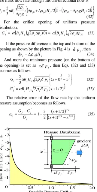
Error in the assumption of uniform pressure distribution for the uni-directional flow in an opening
The error of the rate of uni-directional flow through an opening should be estimated first of all when the pressure gradient is neglected. The density difference between the adjacent rooms and the density through j-th opening of dimensions in Hj×Bj (=Aj) is expressed as
) 0 (>
∆ρj and
ρ
jrespectively. If the static pressure at the middle height (z = 0 ) of the opening is ∆pj0, then the vertical pressure distribution in the opening is as follows.The mass flow rate through this uni-directional flow is
(32) For the orifice opening of uniform pressure distribution,
If the pressure difference at the top and bottom of the opening as shown by the picture in Fig. 4 is δ pj, then And more the minimum pressure (on the bottom of the opening) is set as xδ pj, then Eqs. (32) and (33) becomes as follows.
The relative error of the flow rate by the uniform pressure assumption becomes as follows.
Figure 4. Flow Rate Error by the Uniform Pressure
This equation imply that the error of the flow rate depends only the specific pressure drift x and the function
) (x
G
ε is shown in Fig. 4. The maximum error is
From this result, the uniform pressure assumption in the opening becomes to overlook the flow rate up to maximum 6 %. The error like to this extent may be allowed in the ventilation calculation by the uni- directional flow network model.
Stack Ventilation in One-story House
Using the single room stack ventilation as shown in Fig. 5, the effect of the consideration of bi-directional flows in openings is examined.
The calculation conditions are shown in Fig. 5. The room temperature is fixed to 20 °C and the heat enough for the temperature is supplied. Three kinds of ventilation calculation methods are examined, (i) by the gradient pressure distribution and the flow rates by Eq. (32), (ii) by the uniform pressure and flow rates by Eq.(33) and (iii) by the modified network model using the circulation flow included in Eq. (29).
The calculation results are shown in Fig. 6. The errors in flow rates and the heat supply rates are compared in each other. In Case (i) being the basis of the comparison, the neutral plane exists in 1st opening (hen= 1.37 m) and so the bi-directional flows may occur. The heat supply rate to keep the room temperature 20 °C is 19.2 kW. Total ventilation rate is 57.4 kg/min.
By the calculation of Case (ii) with uniform pressure distributions, the flow in 1st opening is a uni-directional as a matter of course. The flow rates based on the assumption of uniform pressure are overestimated as mentioned above (as shown in Fig. 4) and so the flow rate of 46.7 kg/min in 2nd opening in Fig. 6(ii) is over the standard value of 40 kg/min in the figure 6(i). But the heat supply rate is 18.5% less than the Case (i) because the total ventilation rate is 46.7 kg/min being less than Case(i).
By the calculation of Case(iii) with the modified method, the same bi-directional flows in 1st opening are reproduced as the ventilation in Case(i). The total ventilation rate is 61.5 kg/min and the heat supply rate is 20.6 kW, and so the error is allowable value of 7.2 % and this is less than 18.5% in Case (ii).
Figure 5. Ventilation model by one-story house
j p δ j p xδ j g∆ρ 3 / 0819 . 0 kg m = ∆ρ
C
°
0
C
°
20
6
.
0
=
α
1,000 x1,000H W Window Door Stairwell Door 2,000 x1,000H W 1,000 x1,000B W 2, 000 1 ,000 3, 0 00 3 ,000 Window Skylight Heat Source 100kW Insulated Walls Calm 1, 000 A= 15 m2 Neutral Plane hn= 1,368 mm Neutral Plane hn= 1,443 mm Neutral Plane hn= 1,189 mm (19.2 kW, = -) (20.6 kW, = 7.2 %) (15.7 kW, = -18.5 % ) 17.4 57.4 40.0 unit: kg/min 46.7 46.7 61.5 14.8 46.7 unit: kg/min (i)Calculation Gradients Pressure by (iii)Calculation Pressure by Uniform Distributions & Bi-directional Flows (ii)Calculation Pressure by Uniform Distributions 1 2 2 1 1 2 31 65 34 108 20 87 20 102 82 Mode A Mode C Mode B 29 25 54 79 2 96 98 25 54 Mode B' Mode A' 3 1 unit: kg/min unit: kg/min unit: kg/min unit: kg/min unit: kg/min
(i)Ordinary (ii) Modified
Network Model Network Model
(Three Modes) (Two Modes)
-50 0 100
Intial Value G , kg/min (Window on Room 2 )2
In tia l V a lu e G , k g /m in (W in d o w o n R o o m 1 ) 1 50 -100 -50 0 50 = 100 kW
Dot Scale= 0.25 kg/min
Mode A Mode C Mode B Solution Solution Solution G2 G1 G6 G1= 0 G2= 0 G6= 0 II III IV 1 2 3 4 1 2 6 I Figure 6. Stack ventilation results in one-story house
Stack Ventilation in Two-story House Installed with a Stairwell
The ventilation characteristics of the ordinary network model permitted the uni-directional flow and the modified model which is allowed for the bi-directional flow are comparatively studied in the case of the stack ventilation in a two-story house installed with a stairwell.
Figure 7 shows the composition of the openings in the house. The stairwell is partitioned into two zones by an imaginary floor with an opening possessing an equivalent flow resistance in the stairwell. The dimensions of the openings are written in Fig.7. The coefficients of flow rate α=0.65 are for the doors and windows and α =0.20 for the resistance in stairwell.
(Nitta,, 2002, Peppes et al, 2002)
The walls are insulated and the outdoor is calm. The room temperatures are not fixed and the heat of 100 kW is supplied to 1st room. The network for this example is previously shown in Fig. 1 and Eqs. (1) – (10)’.
The calculation results are shown in Fig.8. Figure 8(i) is the three kinds of modes obtained under the same conditions for the ordinary network model and Figure 8(ii) shows two kinds of modes calculated with the modified network model. These modes or the plural solutions can be happened from the different initially supposed values of the loop flow rates at the beginning of the numerical calculation. We call a set of the modes the ventilation variety.(Nitta, 1997, 1999, 2001, 2002 )
Figure 7. Ventilation model by two-story house with a stairwell
Figure 8. Ventilation varieties in buoyancy ventilation in the two-story house
Figure 9. Chaos map for the ventilation variety obtained by the ordinary network model in the two-story house
W ε W ε W ε C ° 0 C ° 0 C ° 0 C ° 20 C ° 20 C ° 20 1 ˆ W 1 ˆ W C ° 0 C ° 92 C ° 55 C ° 68 C ° 58 C ° 111 35°C C ° 41 61°C C ° 0 C ° 0 C ° 0 C ° 0 0°C C ° 68 C ° 58 C ° 58 C ° 58 C ° 61 C ° 61
65
.
0
=
α
α
=0.20Door Windows, Door: = 1.3 m Door Door Door Door Door Door Door Skylight Windows Windows 100kW Skylight: = 0.65 m Stairwell: = 3.6 m 2 2 2 3, 000 3, 0 00 3 ,000 Windows 86 83 62 107 90 133 209 166 7 71 102 61 59 60 60 27 138 133 184 88 79 193 15 18 16 51 26 29 99 27 8 13 48 104 147 57 194 140 50 138 124 97 81 54 Mode STAIR
Flow Rate Unit:kg/min
Mode DUCT
Mode BOTH Mode ZERO
Temperature
0 10 20 30 40 50
-3,000 -2,000 -1,000 0 1,000 2,000 3,000
Intial Value (Duct), kg/min
0 In ti a l V a lu e (S ta ir c a se ) ,k g /m in
Dot Scale= 10 kg/min
= 100 kW 2,000 1,000 -1,000 -2,000 (Vent)=0.65 m, 2 (Staircase)= 3.6 m 2 Mode STAIR
Mode BOTH Mode DUCT Mode ZERO
The ventilation variety is a physical fact and may be happened not only by the network model but also by the CFD analysis or the experiments. (Nitta, 2002, Li et al., 2000, 2002) Such the ventilation variety is caused mainly by the variable buoyancy force involved in the fixed heat supply ventilation system. The maximum number of the potential modes is the five times of the independent loop number L. (Nitta 1997)
By the modified network model the bi-directional flows is found on a door faced to the stairwell as shown in Fig. 8(ii). But the bi-directional flow decreased the ventilation modes from three to two. Though Mode A and B corresponded to Mode A’ and B’ respectively, Mode C resulted in Mode A’. It was proved that the bi-directional flows might promote the heat exchange and decrease the number of the ventilation modes.
Figure 9 shows the indication of advent of the various ventilation modes in case of the ordinal network model. Starting the calculation from a certain couple of flow rates on the coordinate (G10, G20), the color corresponding to the resulting mode is assigned on the same coordinate. If the outflow from the windows on the first floor (G10> 0 or first and second quadrants) is expected, the solution reached to Mode A, and if the initial values of the third quadrant (G10 < 0 and G20 > 0 ) is selected, the solution becomes decisively to Mode B. But if the initial values of the fourth quadrant (G10< 0 and G20< 0 ) are set, the mode obtained is not deterministic but probabilistic and the nature of chaos appears. In this figure the lines of G1= 0, G2= 0 and G6 (= G1+G2) = 0 are recognized. This means the strong influence of the combination of flow directions on the formation of mode.
Stack Ventilation in Three-story House Installed with a stairwell and a vertical duct
The ventilation characteristics are also investigated with the three-story house as shown in Fig.10. The stairwell and the duct are partitioned at each floor heights for the network model calculation. The coefficient of flow rate is
65
.
0
=
α
for the doors and windows,α
=
0
.
20
for the stairwell andα
=
∞
(this means no pressure loss) for the duct. And so the numbers of the network is M=16, N=26 and L=10.Figure 10. Ventilation model by three-story house with one stairwell and one vertical duct
Figue 11. Calculation results by ordinary network model
Figure 12. Ventilation modes of three-story house
Figure 13. Chaos map of ventilation modes for three-story house with a stairwell and a duct
Figure 14. Calculation results by modified network model and CFD analysis
Mode BOTH
Mode DUCT Mode STAIR
Mode ZERO
Duct Room Stairwell Duct Room Stairwell Duct Room Stairwell Duct Room Stairwell
84 78 80 22 104 88 131 210 169 10 8 81 106 70 47 83 45 11 63 121 180 168 25 9 12 50 146 CFD Analysis Modified Network Model
∞
=
α
α=0.65 α =0.20 A α A α A α C ° 1 ˆ W A α A α G~Four ventilation modes are obtained for the normal network model as shown in Fig. 11. Figure 12 is the smoke flow patterns when the ventilation is regarded as the fire on the early stage.
Figure 13 shows the chaos map similar to Fig. 9 for the two-story house. In the fourth quadrant, the self similarity of the main feature of chaos was recognizes. The calculation results by the modified network model and CFD analysis for the reference are shown in Fig. 14. (Nitta, 2002) The ventilation variety disappeared and only one mode was obtained in the modified network. The ventilation rates agreed considerably with the CFD results and the validity of the modified network model was confirmed.
The propriety of the proposed modified network model should be done further by experimental works and it is a subject of the research in future.
CONCLUSIONS
The formulations of the multi-room ventilation calculations for the ordinary network model restricted to the uni-directional opening flow and the modified network model allowed for the bi-directional opening flows were established, and the mutual errors of both models in flow rates and the characteristics of the ventilation variety were examined.
For the network models of lumped constant circuits, ventilation rates and room temperatures as unknown variables were expressed, and the incidence matrix and loop matrix familiar in the graph theorem were introduced. The nonlinear ventilation equations were solved by Newton-Raphson successive method according to the Kirchhoff’s second law.
The modified network model was constructed based on the idea that the bi-directional flow might be happened in a few openings near the neutral height of the building and a circulation flow in each opening of the potential bi-directional flow guessed from the solution by the ordinary model was added and only the heat balance equation was modified.
The assumption error of the flow rate by the uniform pressure difference distribution in an opening tacitly used in the network model was allowable value below 6 %. The multi-room stack ventilation system in which the room temperatures are not fixed and only the heat supply rates are designated indicated that the plural solutions (or modes) are commonly get and the ventilation variety holds the probabilistic nature of chaos depending on the initial setting values in spite of the deterministic fundamental equations
The heat exchange effect of the bi-directional flows on the reduction of the plural ventilation modes was ascertained by means of the numerical calculations for one-, two- and three-story houses attached a stairwell.
At last, we want to stress that the stack ventilation system is non-linear and has the nature of chaos, and so the prediction is greatly influenced by the initial values of the numerical calculation.
REFERENCES
Li,Yuguo et al., 2000, "Some Examples of Solution Multiplicity in Natural Ventilation", Roomvent 2000, pp.289-294.
Li,Yuguo et al., 2002, “Some Examples of Solution Multiplicity in Natural Ventilation”, Building & Environment 36, pp.851-858.
Nitta,K., 1994, "Calculation Method of Multi-Room Ventilation", Memoirs Kyoto Institute of Technology 42, pp.59-94.
Nitta,K., 1997, "Analytical Study on a Variety of Forms of Multi-room Ventilation", 5th Int. Symp. on Building & Urban Environment Engineering, pp.67-78.
Nitta,K., 1999, "Variety Modes & Chaos in Smoke Ventilation by Ceiling Chamber System", Proc. 6th Int. IBPSA (BS’99), pp.473-480.
Nitta,K., 2001, "Variety Modes and Similarity in Natural Ventilation", 6th Int. Symp. on Building & Urban Environment Engineering, pp.51-60.
Nitta,K., 2001, "Variety Modes and Chaos in Natural Ventilation or Smoke Venting System, Proc. 7th Int. IBPSA (BS2001), pp.635-642.
Nitta,K., 2003, "Modeling of the Flow Resistance of the
Stairwell on the Ventilation Network Calculation", 2nd Int. Symp. on Building Physics Conference, p.8, ( in Press).
Peitogen,H.O., Jurgens,H. & Saupe,D., 1992, "Chaos and Fractal", Springer-Verlag, pp.774.
Peppes,A.A., Santamouris,M & Asimakopoulos,D.N., 2003, "Experimental Study of Buoyancy-driven Stairwell Flow in a Three-story Building", Building & Environment, 37, pp.497-506.
NOMENCLATURE
A : Area of Opening, (m2) B : Opening Breadth, (m) Cp : Specific Heat of Air, (kJ/ kgK) h : Opening Height, (m) G : Mass Flow Rate, (kg/s)
GB : Mass Flow Rate of Circulation, (kg/s)
g : Gravity Acceleration, (m/s2) L : Independent Loop Number, (-)
p
∆ : Pressure Loss in an opening, (Pa) pw : Wind pressure, (Pa),
T : Absolute Temperature, (K)
U :Overall Heat Transfer Coefficient, (kW/°C) W : Heat Supply Rate, (kW)
α
: Coefficient of Flow Rate, (-)ε
: Error, (-)θ
: Temperature, (°C)ρ
: Density of Air, (kg/m3) [I ] : Incidence Matrix, (-)[L] : Loop (Closed Circuit) Matrix, (-)
[
]
−1 : Inverse Matrix, (*)T
−
]
[
: Transposed Matrix, (*): Diagonalized Square Matrix, (*)
[F] :Boolean Transformation in Temperature, (-) { } : Vector, (*)
{d} : Flow direction Vector, (-)
:Room, O :Opening, :Loop.
Subscript and Superscript ;
B: bi-directional, i :Opening, n :Neutral Plane, o: Outdoor, :Room,