Design of Active Noise Control
Systems With the TMS320
Family
1996
Digital Signal Processing Solutions
Application
Report
If the spine is too narrow to print this text on, reduce ALL spine copy (including TI bug at the top of the spine and the year at the bottom) the same amount and re-position at the reference marks as shown for the blue-line.
If the reduction required is such that the resulting copy is very small, we may opt to print the spine with no text.
Design of Active Noise Control
Systems With the TMS320 Family
Sen M. Kuo, Ph.D.
Issa Panahi, Ph.D.
Kai M. Chung
Tom Horner
Mark Nadeski
Jason Chyan
Digital Signal Processing Products—Semiconductor Group
SPRA042 June 1996
IMPORTANT NOTICE
Texas Instruments (TI) reserves the right to make changes to its products or to discontinue any semiconductor product or service without notice, and advises its customers to obtain the latest version of relevant information to verify, before placing orders, that the information being relied on is current.
TI warrants performance of its semiconductor products and related software to the specifications applicable at the time of sale in accordance with TI’s standard warranty. Testing and other quality control techniques are utilized to the extent TI deems necessary to support this warranty. Specific testing of all parameters of each device is not necessarily performed, except those mandated by government requirements.
Certain applications using semiconductor products may involve potential risks of death, personal injury, or severe property or environmental damage (“Critical Applications”).
TI SEMICONDUCTOR PRODUCTS ARE NOT DESIGNED, INTENDED, AUTHORIZED, OR WARRANTED TO BE SUITABLE FOR USE IN LIFE-SUPPORT APPLICATIONS, DEVICES OR SYSTEMS OR OTHER CRITICAL APPLICATIONS.
Inclusion of TI products in such applications is understood to be fully at the risk of the customer. Use of TI products in such applications requires the written approval of an appropriate TI officer. Questions concerning potential risk applications should be directed to TI through a local SC sales office.
In order to minimize risks associated with the customer’s applications, adequate design and operating safeguards should be provided by the customer to minimize inherent or procedural hazards.
TI assumes no liability for applications assistance, customer product design, software performance, or infringement of patents or services described herein. Nor does TI warrant or represent that any license, either express or implied, is granted under any patent right, copyright, mask work right, or other intellectual property right of TI covering or relating to any combination, machine, or process in which such semiconductor products or services might be or are used.
Content
Title Page
ABSTRACT . . . 1
INTRODUCTION . . . 3
The General Concept of Acoustic Noise Control. . . 3
General Applications of Active Noise Control . . . 4
The Development of Active Techniques for Acoustic Noise Control . . . 5
EVALUATING THE PERFORMANCE OF ANC SYSTEMS . . . 7
TYPES OF ANC SYSTEMS. . . 9
The Broadband Feedforward System. . . 9
The Narrowband Feedforward System . . . 10
The Feedback ANC System . . . 11
The Multiple-Channel ANC System . . . 12
ALGORITHMS FOR ANC SYSTEMs . . . 13
Algorithms for Broadband Feedforward ANC Systems . . . 13
Secondary-Path Effects. . . 14
Filtered-X Least-Mean-Square (FXLMS) Algorithm . . . 15
Leaky FXLMS Algorithm . . . 20
Acoustic Feedback Effects and Solutions (FBFXLMS Algorithm) . . . 20
Filtered-U Recursive LMS (RLMS) Algorithm . . . 24
Algorithms for Narrowband Feedforward ANC Systems . . . 27
Waveform Synthesis Method of Synthesizing the Reference Signal (Essex Algorithm). . . 27
Adaptive Notch Filters . . . 31
Algorithms for Feedback ANC Systems . . . 35
DESIGN OF ANC SYSTEMS . . . 39
System Considerations . . . 39
Sampling Rate and Filter Length . . . 40
Coherence Function . . . 41
Causality . . . 42
Constraints and Solutions . . . 43
Automatic Gain Controller . . . 44
Antialiasing and Reconstruction Analog Filters. . . 45
Analog Interface . . . 46
ANC SYSTEM SOFTWARE . . . 47
Implementation Considerations . . . 47
Quantization Effects in Digital Adaptive Filters . . . 47
Real-Time Software Implementation Process . . . 50
Implementation of Adaptive Filters With the TMS320C25. . . 51
Using the TMS320C2x Simulator to Observe Noise Cancellation . . . 55
PHYSICAL SETUP OF EXPERIMENTAL ANC SYSTEM IN AN ACOUSTIC DUCT . . . 59
OPTIMIZATION OF THE EXPERIMENTAL SYSTEM . . . 61
Determining the Value of µ . . . 61
Determining the Value of LEAKY. . . 63
Determining the Gain of the Preamplifier . . . 64
Single-Tone Sinusoidal Noise Source Case . . . 66
Multiple-Tone Sinusoidal Noise Source Case . . . 69
CONCLUSION . . . 75
REFERENCES. . . 77
Appendixes Title Page APPENDIX A: PSEUDO RANDOM NUMBER GENERATOR . . . 81
APPENDIX B: DIGITAL SINE-WAVE GENERATOR . . . 83
Table Look-Up Method . . . 83
Digital Oscillator . . . 84
APPENDIX C: TMS320C25 ARIEL BOARD IMPLEMENTATION OF ANC ALGORITHMS . . . 85
The Filtered-X LMS Algorithm . . . 85
Filtered-U RLMS Algorithm . . . 95
Filtered-X LMS Algorithm With Feedback Cancellation . . . 107
APPENDIX D: GENERAL CONFIGURABLE SOFTWARE FOR ANC EVALUATION . . . . 121
Configuration File (config.asm) Description . . . 122
ANC Algorithm Module Listing (anc.asm) . . . 127
ANC Linker Command File (anc.cmd) . . . 138
ANC System Configuration File (config.asm). . . 139
TMS320C2x EVM Initialization Command File (evminit.cmd) . . . 141
Global Constants and Variables (globals.asm). . . 141
System Initialization File (init.asm). . . 144
Macro Library File (macros.asm). . . 147
ANC System Supervisor Program (main.asm) . . . 148
Memory Definitions File (memory.asm) . . . 149
Simulation Models and Waveform Generators File (models.asm) . . . 152
Interrupt Vectors and Interrupt Service Routine Traps File (vectors.asm). . . 155
APPENDIX E: SCHEMATIC DIAGRAM OF 8-ORDER BUTTERWORTH LOW-PASS FILTER . . . 157
APPENDIX F: ANC UNIT SYSTEM SETUP AND OPERATION PROCEDURE . . . 159
Hardware . . . 159
Software . . . 159
Operation Procedure. . . 160
APPENDIX G: TMS320C26 DSP STARTER KIT, AN ALTERNATIVE TO THE SPECTRUM ANALYZER . . . 161
List of Illustrations
Figure Title Page
1 Physical Concept of Active Noise Cancellation . . . 4
2 Single-Channel Broadband Feedforward ANC System in a Duct. . . 10
3 Narrowband Feedforward ANC System . . . 10
4 Feedback ANC System . . . 11
5 Multiple-Channel ANC System for a 3-D Enclosure . . . 12
6 System Identification Approach to Broadband Feedforward ANC. . . 14
7 Block Diagram of ANC System Modified to Include H(z) . . . 14
8 Block Diagram of the FXLMS Algorithm for ANC . . . 16
9 Experimental Setup for the Off-Line Secondary-Path Modeling . . . 18
10 Active Noise Control Using the FXLMS Algorithm. . . 19
11 ANC System With Acoustic Feedback Cancellation. . . 21
12 Off-Line Modeling of Secondary and Feedback Paths . . . 22
13 ANC System With the Filtered-U RLMS Algorithm . . . 25
14 Spectrum of Original Noise Signal . . . 27
15 Pole-Zero Placement in z Plane . . . 30
16 Effect of Pole on Notch Bandwidth . . . 31
17 Single-Tone ANC System With Adaptive Notch Filter. . . 32
18 Multiple 2-Weight Adaptive Filters in Parallel . . . 35
19 Block Diagram of the Feedback ANC System . . . 36
20 Probe Tube Used to Increase Coherence . . . 41
21 Microphone Mounting Method to Reduce Flow Turbulence . . . 42
22 ANC System in Duct-Like Machine Chamber . . . 44
23 TMS320C25-Based ANC System Hardware. . . 44
24 Block Diagram of an AGC . . . 45
25 Fixed-Point Arithmetic Model of the LMS Algorithm . . . 48
26 Adaptive Filter Implementation Process . . . 51
27 Memory Layout of Weight Vector and Data Vector . . . 53
28 TMS320C25 Central Arithmetic Logic Unit (CALU) . . . 54
29 The Error Signal Imported From MATLAB . . . 56
30 Error Signal Generated With µ = 2048 . . . 56
31 Experimental Setup of the One-Dimensional Acoustic ANC Duct System . . . 60
32 Level of Attenuation of the Noise Source Versus µ. . . 62
33 Overall Performance as a Function of Equation (95) . . . 63
34 Noise Reduction of System as a Function of LEAKY . . . 64
35 Noise Reduction of the System as a Function of Preamplifier Gain . . . 65
37 Frequency Response of Primary Path P(z) . . . 68
38 Frequency Response of Secondary Path H(z) . . . 68
39 Frequency Response of Feedback Path F(z) . . . 69
40 Error Spectra for FXLMS Algorithm, Noise Source Is a 3-Tone Sinusoid, Order of W(z) = 64, Order of C(z) = 64 . . . 70
41 Error Spectra for FXLMS Algorithm, Noise Source Is a 3-Tone Sinusoid, Order of W(z) = 127, Order of C(z) = 128 . . . 71
42 Error Spectra for FBFXLMS Algorithm, Noise Source Is a 3-Tone Sinusoid, Order of W(z) = 64, Order of C(z) = 64, Order of D(z) = 64 . . . 72
43 Error Spectra for FURLMS Algorithm, Noise Source Is a 3-Tone Sinusoid, Order of A(z) = 63, Order of B(z) = 63, Order of C(z) = 64 . . . 73
44 Pseudo Random Number Generator, 16-Bit Case . . . 81
45 How Constants Are Used in Modeling Acoustic-Channel Transfer Function. . . s126 List of Tables Table Title Page 1 Complexity of Broadband ANC and Narrowband ANC . . . 29
2 Performance of the System as a Function of µ . . . 61
3 Noise Attenuation for a Single-Tone Sinusoidal Noise Source. . . 67
4 Filter Orders for 3-Tone Sinusoidal Noise Source. . . 69
5 Section 1 of the Configuration File . . . 122
6 Section 2 of the Configuration File . . . 123
7 Number of Instruction Cycles, DSP Execution Time, and TMS320C25 DSP Overhead per Algorithm . . . 125
8 How Output Signal Arrays Are Used With Various Algorithms . . . 126
Program Listings Title Page The Filtered-X LMS Algorithm. . . 85
Filtered-U RLMS Algorithm . . . 95
Filtered-X LMS Algorithm With Feedback Cancellation . . . 107
ANC Algorithm Module Listing (anc.asm) . . . 127
ANC Linker Command File (anc.cmd) . . . 138
ANC System Configuration File (config.asm) . . . 139
TMS320C2x EVM Initialization Command File (evminit.cmd) . . . 141
Global Constants and Variables (globals.asm). . . 141
System Initialization File (init.asm). . . 144
Macro Library File (macros.asm) . . . 147
ANC System Supervisor Program (main.asm) . . . 148
Memory Definitions File (memory.asm) . . . 149
Simulation Models and Waveform Generators File (models.asm) . . . 152
ABSTRACT
An active noise control (ANC) system based on adaptive filter theory was developed in the 1980s; however, only with the recent introduction of powerful but inexpensive digital signal processor (DSP) hardware, such as the TMS320 family, has the technology become practical. The specialized DSPs were designed for real-time numerical processing of digitized signals. These devices have enabled the low-cost implementation of powerful adaptive ANC algorithms and encouraged the widespread development of ANC systems. ANC that uses adaptive signal processing implemented on a low-cost, high-performance DSP is an emerging new technology.
This application report presents general background information about ANC methods. Contrasts between passive and active noise control are described, and the circumstances under which ANC is preferable are shown. Different types of noise-control algorithms are discussed: feedforward broadband, feedforward narrowband, and feedback algorithms. The report details the design of a simple ANC system using a TMS320 DSP and the implementation of that design.
INTRODUCTION
The General Concept of Acoustic Noise Control Acoustic noise problems in the environment become more noticeable for several reasons:
•
Increased numbers of large industrial equipments being used: – Engines – Blowers – Fans – Transformers – Compressors – Motors•
The growth of high-density housing increases the population’s exposure to noise because of the proximity to neighbors and traffic•
The use of lighter materials for building and transportation equipment, resulting from cost constraints in construction and fabricationTwo types of acoustic noise exist in the environment. One is caused by turbulence and is totally random. Turbulent noise distributes its energy evenly across the frequency bands. It is referred to as broadband noise, and examples are the low-frequency sounds of jet planes and the impulse noise of an explosion. Another type of noise, called narrowband noise, concentrates most of its energy at specific frequencies. This type of noise is related to rotating or repetitive machines, so it is periodic or nearly periodic. Examples of narrowband noise include the noise of internal combustion engines in transportation, compressors as auxiliary power sources and in refrigerators, and vacuum pumps used to transfer bulk materials in many industries.
There are two approaches to controlling acoustic noise: passive and active. The traditional approach to acoustic noise control uses passive techniques such as enclosures, barriers, and silencers to attenuate the undesired noise. Passive silencers use either the concept of impedance change caused by a combination of baffles and tubes to silence the undesired sound (reactive silencers) or the concept of energy loss caused by sound propagation in a duct lined with sound-absorbing material to provide the silencing (resistive silencers). Reactive silencers are commonly used as mufflers on internal combustion engines, while resistive silencers are used mostly for duct-borne fan noise. These passive silencers are valued for their high attenuation over a broad frequency range. However, they are relatively large, costly, and ineffective at low frequencies, making the passive approach to noise reduction often impractical. Furthermore, these silencers often create an undesired back pressure if there is airflow in the duct.
In an effort to overcome these problems, considerable interest has been shown in active noise control. The active noise control system contains an electroacoustic device that cancels the unwanted sound by generating an antisound (antinoise) of equal amplitude and opposite phase. The original, unwanted sound and the antinoise acoustically combine, resulting in the cancellation of both sounds. Figure 1 shows the waveforms of the unwanted noise (the primary noise), the canceling noise (the antinoise), and the residual noise that results when they superimpose. The effectiveness of cancellation of the primary noise depends on the accuracy of the amplitude and phase of the generated antinoise.
Antinoise Waveform
Residual Noise Primary Noise Waveform
+ =
Figure 1. Physical Concept of Active Noise Cancellation
General Applications of Active Noise Control
The successful application of active control is determined on the basis of its effectiveness compared with passive attenuation techniques. Active attenuation is an attractive means to achieve large amounts of noise reduction in a small package, particularly at low frequencies (below 600 Hz). At low frequencies, where lower sampling rates are adequate and only plane wave propagation is allowed, active control offers real advantages.
From a geometric point of view, active noise control applications can be classified in the following four categories:
•
Duct noise: one-dimensional ducts such as ventilation ducts, exhaust ducts, air-conditioning ducts, pipework, etc.•
Interior noise: noise within an enclosed space•
Personal hearing protection: a highly compacted case of interior noise•
Free space noise: noise radiated into open spaceSpecific applications for active noise control now under development include attenuation of unavoidable noise sources in the following end-equipment:
•
Automotive (car, van, truck, earth-moving machine, military vehicle)– Single-channel (one-dimensional) systems: Electronic muffler for exhaust system, induction system, etc.
– Multiple-channel (three-dimensional) systems: Noise attenuation inside passenger compartment and heavy-equipment operator cabin, active engine mount, hands-free cellular phone, etc.
•
Appliance– Single-channel systems: Air conditioning duct, air conditioner, refrigerator, washing machine, furnace, dehumidifier, etc.
– Multiple-channel systems: Lawn mower, vacuum cleaner, room isolation (local quiet zone), etc.
•
Industrial: fan, air duct, chimney, transformer, blower, compressor, pump, chain saw, wind tunnel, noisy plant (at noise sources or many local quiet zones), public phone booth, office cubicle partition, ear protector, headphones, etc.The algorithms developed for active noise control can also be applied to active vibration control. Active vibration control can be used for isolating the vibrations from a variety of machines and to stabilizing various platforms in the presence of vibration disturbances. As the performance and reliability continue to improve and the initial cost continues to decline, active systems may become the preferred solution to a variety of vibration-control problems.
The Development of Active Techniques for Acoustic Noise Control
Active noise control is developing rapidly because it permits significant improvements in noise control, often with potential benefits in size, weight, volume, and cost of the system. The book Active Control of Sound [1] provides detailed information on active noise control with an emphasis on the acoustic point of view.
The design of an active noise canceler using a microphone and an electronically driven loudspeaker to generate a canceling sound was first proposed and patented by Lueg in 1936 [2]. While the patent outlined the basic idea of ANC, the concept did not have real-world applications at that time. Because the characteristics of an acoustic noise source and the environment are not constant, the frequency content, amplitude, phase, and velocity of the undesired noise are nonstationary (time varying). An active noise control system must be adaptive in order to cope with these changing characteristics.
In the field of digital signal processing, there is a class of adaptive systems in which the coefficients of a digital filter are adjusted to minimize an error signal (the desired signal minus the actual signal; the desired signal is typically defined to be zero). A duct-noise cancellation system based on adaptive filter theory was developed by Burgess in 1981 [3]. Later in the 1980s, research on active noise control was dramatically affected by the development of powerful DSPs and the development of adaptive signal processing algorithms [4]. The specialized DSPs were designed for real-time numerical processing of digitized signals. These devices enabled the low-cost implementation of powerful adaptive algorithms [5] and encouraged the widespread development and application of active noise control systems based on digital adaptive signal processing technology.
Many modern active noise cancelers rely heavily on adaptive signal processing—without adequate consideration of the acoustical elements. If the acoustical design of the system is not optimized, the digital controller may not be able to attenuate the undesired noise adequately. Therefore, it is necessary to understand the acoustics of the installation and to design the system to assist the adaptive active noise controller to carry out its work. For electrical engineers involved in the development of active control systems, Nelson’s book [1] provides an excellent introduction to acoustics from the active noise control point of view.
EVALUATING THE PERFORMANCE OF ANC SYSTEMS
Analysis of the performance of a given DSP-based controller for different types of source noise and different ANC algorithms is an integral part of successful and optimal design methodology.
An approach to adaptive ANC performance analysis that involves a hierarchy of techniques, starting with an ideal simplified problem and progressively adding practical constraints and other complexities, was developed by Morgan [8]. Performance analysis provides answers to the following questions:
•
What are the fundamental performance limitations?•
What are the practical constraints that limit performance?•
How is performance balanced against complexity?•
What is a practical design architecture?To aid in answering these questions, four levels of performance analysis are defined:
•
Level I derives fundamental performance limits, given continuous measurements over the entire performance surface.•
Level II adds the practical constraint of a fixed number of sensors at discrete locations.•
Level III incorporates knowledge of the transfer function structure between sensor(s) and activator(s).•
Level IV adds in all of the other practical effects and design constraints required for detailed performance calculations.At each step, a degree of confidence is gained and a benchmark is established for comparison and cross-checking with the next level of complexity.
The principle of ANC is simple; however, when it is applied in the real world, the following questions must be answered [9]:
•
Which algorithm should be adopted?•
Where should speakers and microphones be located?•
How is the flow noise (the noise of air passing over the surface of the microphone) going to be reduced?•
How is the power of the speakers going to be increased?•
How is the durability of the microphones and the speakers going to be increased?•
How is the cost of the hardware (controller, microphone, and speaker) going to be reduced? To be suitable for industrial or commercial use, the ANC system must have certain properties [10]:•
Maximum efficiency over the desired frequency band•
Autonomy with regard to the installation (the system could be built and preset at the time of manufacture and then installed on site)•
Self-adaptability of the system to deal with any variations in the physical parameters (temperature, airflow, etc.)•
Robustness and reliability of the elements of the system and simplification of the control electronicsThe continuous progress of active noise control involves the development of improved adaptive signal processing algorithms, transducers, and digital signal processing hardware. More sophisticated adaptive
filtering algorithms allow faster convergence (the equalization of the phase and magnitude of the undesired noise and the antinoise so that cancellation occurs), greater noise attenuation, and are more resistant to interference. The DSP hardware implementation allows these more sophisticated algorithms to be applied in real time to improve system performance.
TYPES OF ANC SYSTEMS
Broadband noise cancellation requires knowledge of the noise source (the primary noise) in order to generate the antinoise signal. The measurement of the primary noise is used as a reference input to the noise canceler. Primary noise that correlates with the reference input signal is canceled downstream of the noise generator (a loudspeaker) when phase and magnitude are correctly modeled in the digital controller. For narrowband noise cancellation (reduction of periodic noise caused by rotational machinery), active techniques have been developed that are very effective and that do not rely on causality (having prior knowledge of the noise signal). Instead of using an input microphone, a tachometer signal provides information about the primary frequency of the noise generator. Because all of the repetitive noise occurs at harmonics of the machine’s basic rotational frequency, the control system can model these known noise frequencies and generate the antinoise signal. This type of control system is desirable in a vehicle cabin, because it will not affect vehicle warning signals, radio performance, or speech, which are not normally synchronized with the engine rotation.
Active noise control systems are based on one of two methods. Feedforward control is where a coherent reference noise input is sensed before it propagates past the canceling speaker. Feedback control [6, 7] is where the active noise controller attempts to cancel the noise without the benefit of an upstream reference input.
Feedforward ANC systems are the main techniques used today. Systems for feedforward ANC are further classified into two categories:
•
Adaptive broadband feedforward control with an acoustic input sensor•
Adaptive narrowband feedforward control with a nonacoustic input sensor The Broadband Feedforward SystemA considerable amount of broadband noise is produced in ducts such as exhaust pipes and ventilation systems. A relatively simple feedforward control system for a long, narrow duct is illustrated in Figure 2. A reference signal x(n) is sensed by an input microphone close to the noise source before it passes a loudspeaker. The noise canceler uses the reference input signal to generate a signal y(n) of equal amplitude but 180° out of phase. This antinoise signal is used to drive the loudspeaker to produce a canceling sound that attenuates the primary acoustic noise in the duct.
The basic principle of the broadband feedforward approach is that the propagation time delay between the upstream noise sensor (input microphone) and the active control source (speaker) offers the opportunity to electrically reintroduce the noise at a position in the field where it will cause cancellation. The spacing between the microphone and the loudspeaker must satisfy the principles of causality and high coherence, meaning that the reference must be measured early enough so that the antinoise signal can be generated by the time the noise signal reaches the speaker. Also, the noise signal at the speaker must be very similar to the measured noise at the input input microphone, meaning the acoustic channel cannot significantly change the noise. The noise canceler uses the input signal to generate a signal y(n) that is of equal amplitude and is 180° out of phase with x(n). This noise is output to a loudspeaker and used to cancel the unwanted noise.
Controller ANC x(n)
y(n)
e(n) Error Microphone Input Microphone Noise Primary Noise Source Canceling Speaker L
Figure 2. Single-Channel Broadband Feedforward ANC System in a Duct
The error microphone measures the error (or residual) signal e(n), which is used to adapt the filter coefficients to minimize this error. The use of a downstream error signal to adjust the adaptive filter coefficients does not constitute feedback, because the error signal is not compared to the reference input. Actual implementations require additional considerations to handle acoustic effects in the duct. These considerations are discussed in the section Algorithms for ANC Systems, page 13.
The Narrowband Feedforward System
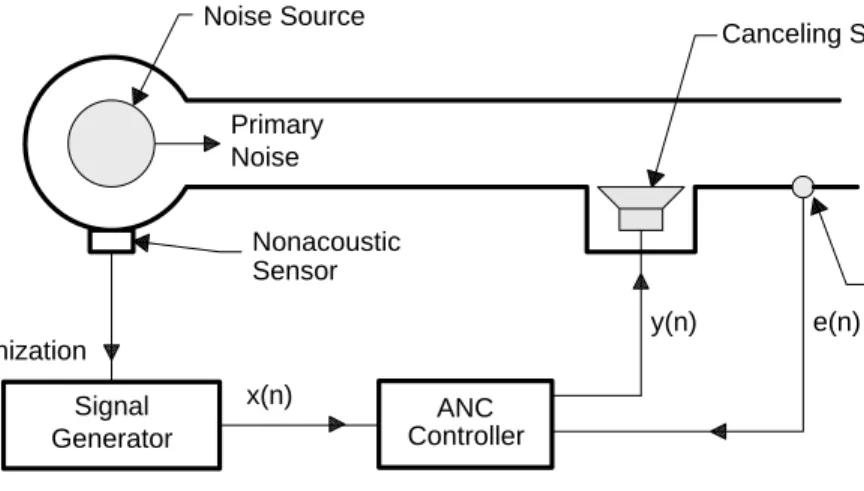
In applications where the primary noise is periodic (or nearly periodic) and is produced by rotating or reciprocating machines, the input microphone can be replaced by a nonacoustic sensor such as a tachometer, an accelerometer, or an optical sensor. This replacement eliminates the problem of acoustic feedback (described in the subsection Acoustic Feedback Effects and Solutions, page 20).
The block diagram of a narrowband feedforward active noise control system is shown in Figure 3. The nonacoustic sensor signal is synchronous with the noise source and is used to simulate an input signal that contains the fundamental frequency and all the harmonics of the primary noise. This type of system controls harmonic noises by adaptively filtering the synthesized reference signal to produce a canceling signal. In many cars, trucks, earth moving vehicles, etc., the revolutions per minute (RPM) signal is available and can be used as the reference signal. An error microphone is still required to measure the residual acoustic noise. This error signal is then used to adjust the coefficients of the adaptive filter.
Sensor Nonacoustic Generator Signal x(n) y(n) e(n) Error Microphone Noise Primary Noise Source Canceling Speaker Synchronization Controller ANC
Generally, the advantage of narrowband ANC systems is that the nonacoustic sensors are insensitive to the canceling sound, leading to very robust control systems. Specifically, this technique has the following advantages:
•
Environmental and aging problems of the input microphone are automatically eliminated. This is especially important from the engineering viewpoint, because it is difficult to sense the reference noise in high temperatures and in turbulent gas ducts like an engine exhaust system.•
The periodicity of the noise enables the causality constraint to be removed. The noise waveform frequency content is constant. Only adjustments for phase and magnitude are required. This results in more flexible positioning of the canceling speaker and allows longer delays to be introduced by the controller.•
The use of a controller-generated reference signal has the advantage of selective cancellation; that is, it has the ability to control each harmonic independently.•
It is necessary to model only the part of the acoustic plant transfer function relating to the harmonic tones. A lower-order FIR filter can be used, making the active periodic noise control system more computationally efficient.•
The undesired acoustic feedback from the canceling speaker to the input microphone [16] is avoided.The Feedback ANC System
Feedback active noise control was proposed by Olson and May in 1953 [6]. In this scheme, a microphone is used as an error sensor to detect the undesired noise. The error sensor signal is returned through an amplifier (electronic filter) with magnitude and phase response designed to produce cancellation at the sensor via a loudspeaker located near the microphone. This configuration provides only limited attenuation over a restricted frequency range for periodic or band-limited noise. It also suffers from instability, because of the possibility of positive feedback at high frequencies. However, due to the predictable nature of the narrowband signals, a more robust system that uses the error sensor’s output to predict the reference input has been developed (see Figure 4). The regenerated reference input is combined with the narrowband feedforward active noise control system.
ANC Controller y(n) e(n) Error Microphone Noise Primary Noise Source Canceling Speaker
Figure 4. Feedback ANC System
One of the applications of feedback ANC recognized by Olson [7] is controlling the sound field in headphones and hearing protectors [27]. In this application, a system reduces the pressure fluctuations in the cavity close to a listener’s ear. This application has been developed and made commercially available.
The Multiple-Channel ANC System
Many applications can display complex modal behavior. These applications include:
•
Active noise control in large ducts or enclosures•
Active vibration control on rigid bodies or structures with multiple degrees of freedom•
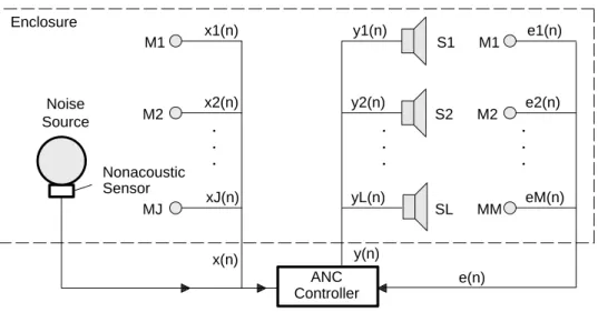
Active noise control in passenger compartments of aircraft or automobilesWhen the geometry of the sound field is complicated, it is no longer sufficient to adjust a single secondary source to cancel the primary noise using a single error microphone. The control of complicated acoustic fields requires both the exploration and development of optimum strategies and the construction of an adequate multiple-channel controller. These tasks require the use of a multiple-input multiple-output adaptive algorithm. The general multiple-channel ANC system involves an array of sensors and actuators. A block diagram of a multiple-channel ANC system for a three-dimensional application is shown in Figure 5. e(n) y(n) x(n) Sensor Nonacoustic eM(n) e2(n) e1(n) SL S2 S1 yL(n) y2(n) y1(n) xJ(n) x2(n) x1(n) MM M2 M1 Enclosure MJ M2 M1 Source Noise . . . . . . . . . ANC Controller
ALGORITHMS FOR ANC SYSTEMS This section discusses the algorithms used in three kinds of ANC systems:
•
Broadband feedforward ANC systems that use acoustic sensor (microphone) input•
Narrowband feedforward ANC systems that use nonacoustic sensor input•
Feedback ANC systems that use only an error sensor Adaptive filters can be realized as:•
Transversal—finite impulse response (FIR)•
Recursive—infinite impulse response (IIR)•
Lattice filters•
Transform-domain filtersThe most common algorithm applied to adaptive filters is the transversal filter using the least mean-squared (LMS) algorithm. The residual noise can be used as an error signal input to an adaptive algorithm that adjusts the filter coefficients to model (estimate) the acoustic-channel effects.
Algorithms for Broadband Feedforward ANC Systems
Broadband active noise control can be described in a system identification framework, as shown in Figure 6. Using a digital frequency-domain representation of the problem, the ideal active noise control system uses an adaptive filter W(z) to estimate the response of an unknown primary acoustic path P(z) between the reference input sensor and the error sensor. The z-transform of e(n) can be expressed as:
E(z)+ D(z) ) Y(z) + X(z)[P(z) ) W(z)] (1)
where E(z) is the error signal, X(z) is the input signal, and Y(z) is the adaptive filter output. After the adaptive filter W(z) has converged, E(z) + 0. Equation (1) becomes:
W(z)+ –P(z) (2)
which implies that:
y(n)+ –d(n) (3)
Therefore, the adaptive filter output y(n) has the same amplitude but is 180° out of phase with the primary noise d(n). When d(n) and y(n) are acoustically combined, the residual error becomes zero, resulting in cancellation of both sounds based on the principle of superposition.
x(n) y(n) d(n) e(n) Duct Acoustic LMS W(z) System P(z) Unknown ANC Controller
Input Microphone Error Microphone
e(n)
Figure 6. System Identification Approach to Broadband Feedforward ANC Secondary-Path Effects
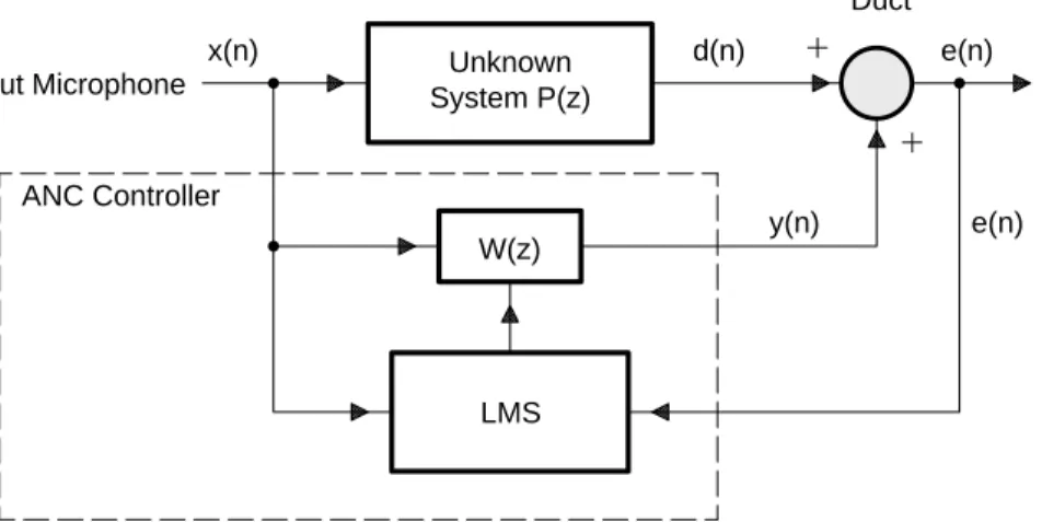
The error signal e(n) is measured at the error microphone downstream of the canceling speaker. The summing junction in Figure 6 represents the acoustical environment between the canceling speaker and the error microphone, where the primary noise d(n) is combined with the antinoise y(n) output from the adaptive filter. The antinoise signal can be modified by the secondary-path function H(z) in the acoustic channel from y(n) to e(n), just as the primary noise is modified by the primary path P(z) from the noise source to the error sensor. Therefore, it is necessary to compensate for H(z). A more detailed block diagram of an active noise control system that includes the secondary path H(z) is shown in Figure 7.
P(z) H(z) x(n) y(n) d(n) e(n) Duct Acoustic LMS W(z) ANC Controller e(n)
From Figure 7, the z-transform of error signal e(n) is:
E(z)+ X(z) P(z) ) X(z) W(z) H(z) (4)
Assuming that W(z) has sufficient order, after the convergence of the adaptive filter, the residual error is zero (that is, E(z) + 0). This result requires W(z) to be:
W(z)+–P(z)
H(z) (5)
to realize the optimal transfer function.
Thus, the adaptive filter W(z) has to model the primary path P(z) and inversely model the secondary path H(z). However, it is impossible to invert the inherent delay caused by H(z) if the primary path P(z) does not contain a delay of at least equal length. This is the overall limiting causality constraint in broadband feedforward control systems. Furthermore, from equation (5), the control system is unstable if there is a frequency ω such that H(ω)+ 0. Also, the control system is ineffective if there is a frequency ω where P(ω) + 0, (that is, a zero in the primary path causes an unobservable control frequency). Therefore, the characteristics of the secondary path H(z) have significant effects on the performance of an ANC system. Filtered-X Least-Mean-Square (FXLMS) Algorithm
To account for the effects of the secondary-path transfer function H(z), the conventional least-mean-square (LMS) algorithm [4] needs to be modified [3]. To ensure convergence of the algorithm, the input to the error correlator is filtered by a secondary-path estimate C(z). This results in the filtered-X LMS (FXLMS) algorithm developed by Morgan [11]. Burgess [3] has suggested using this FXLMS algorithm to compensate for the effects of the secondary path in ANC applications.
The FXLMS algorithm is illustrated in Figure 8, where the output y(n) is computed as: y(n)+ wT(n)x(n) +
ȍ
N – 1 i+ 0
wi(n)x(n – i) (6)
where wT(n) + [w0(n) w1(n) … wN – 1 (n)]T is the coefficient vector of W(z) at time n and
x (n) + [x(n) x(n – 1) … x(n – N + 1)]Tis the reference signal vector at time n.
The filter is implemented on a DSP in the form: y(n)+
ȍ
N – 1 i+ 0
y′(n) x′(n) C(z) P(z) H(z) x(n) y(n) d(n) e(n) Duct Acoustic LMS W(z) ANC Controller
Figure 8. Block Diagram of the FXLMS Algorithm for ANC The FXLMS algorithm can be expressed as:
w(n) 1) + w(n) – me(n)x(n)h(n) (7)
where µ is the step size of the algorithm that determines the stability and convergence of the algorithm and h(n) is the impulse response of H(z). Therefore, the input vector x(n) is filtered by H(z) before updating the weight vector. However, in practical applications, H(z) is unknown and must be estimated by the filter, C(z). Therefore: (8) wi(n) 1) + wi(n) – me(n)xȀ(n – i) i+ 0, 1 ,..., N – 1 and: (9) w(n) 1) + w(n) – me(n)xȀ(n) where: xȀ(n) + cTx(n) +
ȍ
M – 1 i+0 cix(n – i) (10)is the vector for the filtered version of reference input x′(n) that is computed as:
(11) xȀ(n) + [xȀ(n) xȀ(n – 1) AAA xȀ(n – N ) 1)]T
and:
(12) c+ [c0c1 AAA CM–1]
T
is the coefficient vector of the secondary-path estimate, C(z).
When this algorithm is implemented, the convergence of the filter can be achieved much more quickly than theory suggests, and the algorithm appears to be very tolerant of errors made in the estimation of the secondary path H(z) by the filter C(z). As shown by Morgan [11], the algorithm still converges with nearly 90° of phase error between C(z) and H(z).
It is important that in equation (7), a minus sign is used for ANC applications instead of a plus sign as in a conventional LMS algorithm. This is because the error signal in an ANC system is e(n) + d(n) + y′(n), due to the fact that the residual error e(n) is the result of acoustic superposition (addition) instead of electrical subtraction.
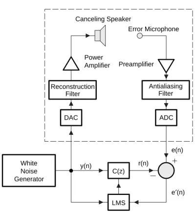
The transfer function H(z) is unknown and is time-varying due to effects such as aging of the loudspeaker, changes in temperature, and air flow in the secondary path. Thus, several on-line modeling techniques were developed by Eriksson [12]. Assuming the characteristics of H(z) are unknown but time-invariant, an off-line modeling technique can be used to estimate H(z) during a training stage. At the end of training, the estimated model C(z) is fixed and used for active noise control. The experimental setup for the direct off-line system modeling is shown in Figure 9, where an uncorrelated white noise is internally generated by the DSP. The training procedure is summarized following the figure. The algorithm of the white noise generator is given in Appendix A, Pseudo Random Number Generator.
H(z) Path Secondary e′(n) e(n) r(n) y(n) ADC Antialiasing Filter LMS C(z) DAC Reconstruction Filter Canceling Speaker Error Microphone Preamplifier Amplifier Power Generator Noise White
Figure 9. Experimental Setup for the Off-Line Secondary-Path Modeling
1. Generate a sample of white noise y(n) using the algorithm given in Appendix A. Output y(n) to drive the canceling loudspeaker. This internally generated white noise is used as the reference input for the adaptive filter C(z) and the LMS coefficient adaptation algorithm.
2. Input the secondary-path response e(n) from the error microphone. 3. Compute the response of the adaptive model r(n):
(13) r(n)+
ȍ
M – 1 i+0
ci(n) y(n – i)
where ci(n) is the ith coefficient of the adaptive filter C(z) at time n and M is the order of filter.
4. Compute the difference:
(14) eȀ(n) + e(n) – r(n)
5. Update the coefficients of the adaptive filter C(z) using the LMS algorithm:
(15) ci(n) 1) + ci(n)) meȀ(n)y(n – i), i + 0, 1,..., M – 1
where µ is the step size that must satisfy the following stability condition:
(16) 0t m t 1
M Py
where Py is the power of the generated white noise y(n).
6. Repeat the procedure for about 10 seconds. Save the coefficients of the adaptive filter C(z) and use them in the following noise cancellation mode.
After the off-line modeling is completed, the system is operated in the active noise cancellation mode. The algorithm is illustrated in Figure 10, and the procedure of on-line noise control is summarized following the figure. Primary Noise Input Microphone C(z) y(n) e(n) LMS W(z) x(n) Error Microphone Canceling Speaker ANC Controller
Figure 10. Active Noise Control Using the FXLMS Algorithm
1. Input the reference signal x(n) (from the input microphone) and the error signal e(n) (from the error microphone) from the input ports.
2. Compute the antinoise y(n):
(17) y(n)+
ȍ
N – 1 i+0
wi(n) x (n – i)
where wi(n) is the ith coefficient of the adaptive filter W(z) at time n and N is the order of filter
w(z).
4. Compute the filtered-X version of x′(n): xȀ(n) +
ȍ
M i+0
cix (n – 1) (18)
5. Update the coefficients of adaptive filter W(z) using the FXLMS algorithm:
wi(n) 1) + wi(n) – me(n)xȀ(n – i), i + 0, 1,..., N – 1 (19)
6. Repeat the procedure for the next iteration. Note that the total number of memory locations required for this algorithm is 2(N + M) plus some parameters.
Assembly language implementations of the FXLMS algorithm are given in Appendix C, TMS320C25 Ariel Board Implementation of ANC Algorithms, and Appendix D, General Configurable Software for ANC Evaluation.
Leaky FXLMS Algorithm
When an adaptive filter is implemented on a signal processor with fixed word lengths, roundoff noise is fed back to the filter weights and accumulates continuously. This can cause the coefficients to grow larger than the dynamic range of the processor (overflow), which results in inaccurate filter performance. One solution to the problem is based on adding a small forcing function, which tends to bias each filter weight toward zero. According to equation (9), this leaky FXLMS algorithm can be expressed as [5]:
w(n) 1) + vw(n) – me(n)xȀ(n) (20)
where v (the leakage factor) is slightly less than 1 and x′(n) is defined in equation (11).
The leaky FXLMS algorithm can not only reduce numerical error in the finite precision implementation but also limit the output power of the loudspeaker to avoid nonlinear distortion, which is caused by overdriving the canceling speaker.
Acoustic Feedback Effects and Solutions (FBFXLMS Algorithm)
Referring again to the simple system shown in Figure 2 on page 10, the antinoise output to the loudspeaker not only cancels acoustic noise downstream, but unfortunately, it also radiates upstream to the input microphone, resulting in a contaminated reference input x(n). This acoustic feedback introduces a feedback loop or poles in the response of the model and results in potential instability in the control system. This problem has been intensively studied in active noise and vibration control literature. Solutions such as the following have been proposed:
1. Using directional microphones and speakers [14]. (This has a limitation in that directional arrays are usually highly dependent on the spacing of the array elements and are directional over only a relatively narrow frequency range.)
2. Using fixed compensating signals (generated from the compensating filter whose coefficients are determined off-line by using a training signal) to cancel the effects of the acoustic feedback 3. Using a second off-line adaptive filter in parallel with the feedback path [15]
4. Using an adaptive IIR filter [16]
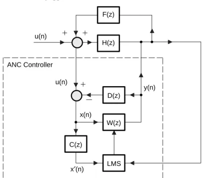
This report examines methods 2 and 4. An adaptive feedforward controller with feedback compensation is shown in Figure 11. The filter D(z) is an estimate of the feedback path F(z) from the adaptive filter output
y(n) to the output of the reference input microphone u(n). Filter D(z) removes the acoustic feedback from the reference sensor input; the filter C(z) compensates the secondary-path transfer function H(z) in the FXLMS algorithm. Removal of the acoustic feedback from the reference input adds a considerable margin of stability to the system if the model D(z) is accurate. The models C(z) and D(z) can be estimated simultaneously by an off-line modeling technique using an internally generated white noise.
The expressions for the antinoise y(n), filtered-X signal x′(n), and the adaptation equation for the FBFXLMS algorithm are the same as that for the FXLMS ANC system, except that x(n) in FBFXLMS algorithm is a feedback-free signal that can be expressed as:
x (n)+ u(n) –
ȍ
L i+1
diy(n – i) (21)
where u(n) is the signal from input microphone, di is the ith coefficient of D(z), and L is the order of D(z).
In the case of a perfect model of the feedback path (that is, D(z) + F(z)), the acoustic feedback is completely canceled by D(z). The adaptive filter converges to the transfer function given in equation (5), the ideal case without acoustic feedback. The function of D(z) is similar to the acoustic echo cancellation that is used in teleconferencing applications [16].
x′(n) e(n) y(n) x(n) u(n) C(z) LMS W(z) D(z) ANC Controller H(z) u(n) F(z)
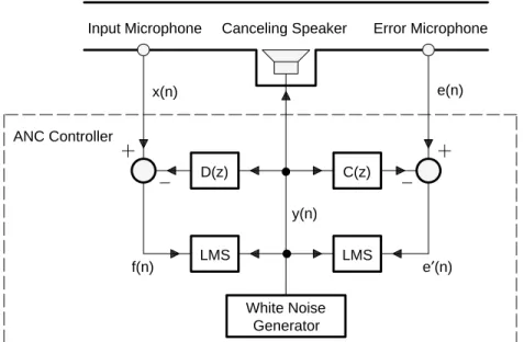
The system performs the off-line modeling first to estimate the secondary-path transfer function H(z) from the canceling speaker to the error microphone and the feedback path transfer function F(z) from the canceling speaker to the input microphone. The off-line modeling algorithm is illustrated in Figure 12 and the procedure is summarized following the figure.
e′(n) Generator White Noise x(n) y(n) C(z) D(z) LMS f(n) e(n) Error Microphone Canceling Speaker Input Microphone LMS ANC Controller
Figure 12. Off-Line Modeling of Secondary and Feedback Paths 1. a. Generate a white noise sample y(n).
b. Output this excitation signal y(n) to drive the canceling loudspeaker. c. Send y(n) to the adaptive filters C(z) and D(z).
d. Send y(n) to the LMS algorithm for updating C(z) and D(z).
2. Input x(n) from the input microphone and e(n) from the error microphone. 3. Compute e′(n) and f(n): (22) eȀ(n) + e(n) –
ȍ
M – 1 i+0 ci(n) y(n – i) and (23) f(n)+ x(n) –ȍ
L – 1 j+0 dj(n) y(n – j)4. Update the coefficients of the adaptive filters C(z) and D(z) using the LMS algorithm: (24) ci(n) 1) + ci(n)) meȀ(n)y(n – i), i + 0, 1,..., M – 1 and (25) dj(n) 1) + dj(n)) mf(n)y(n – j), j + 0, 1,..., L – 1
5. Repeat the off-line modeling for about 10 seconds. Save the coefficients of adaptive filters C(z) and D(z) and use them in the following active noise cancellation mode.
After the off-line modeling, the ANC system is operated in active noise cancellation mode. The algorithm (illustrated in Figure 11) is summarized as follows:
1. Input u(n) and e(n) from the input ports. 2. Compute the feedback-free reference input x(n):
(26) x(n)+ u(n) –
ȍ
L – 1 j+0
diy(n – j)
3. Compute the antinoise y(n):
(27) y(n)+
ȍ
N – 1 i+1
wi(n) x(n – i)
where wi(n) is the ith coefficient of the adaptive filter W(z) at time n and N is the order of filter
W(z).
4. Output the antinoise y(n) to the output port to drive the canceling loudspeaker. 5. Compute the filtered-X version of x′(n):
(28) xȀ(n) +
ȍ
M i+0
cix (n – i)
6. Update the coefficients of adaptive filter W(z) using the following FXLMS algorithm: (29) wi(n) 1) + wi(n)) me(n)xȀ(n – i), i + 0, 1,..., N – 1
7. Repeat the algorithm for the next iteration. Note that the total number of memory locations required in this algorithm is 2(N + M + L) plus some parameters.
Assembly language implementations of this algorithm are given in Appendix C, TMS320C25 Ariel Board Implementation of ANC Algorithms, and Appendix D, General Configurable Software for ANC Evaluation.
Filtered-U Recursive LMS (RLMS) Algorithm
The adaptive infinite impulse response (IIR) filter (method 4 on page 20) was proposed by Eriksson [17] for use in active noise control. This approach considers the acoustic feedback as a part of the whole acoustic plant, and the poles introduced by the acoustic feedback are removed by the poles of the adaptive IIR filter. This control system dynamically tracks changes in the secondary and feedback paths during cancellation operations. Also, as shown in equation (5), the IIR structure has the ability to model transfer functions directly with poles and zeros. Although there are various adaptive IIR algorithms that can be used, the recursive LMS (RLMS) algorithm developed by Feintuch [18] is selected here for reasons of computational simplicity.
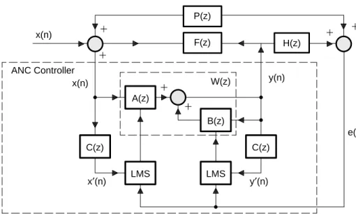
The RLMS algorithm must also be modified to compensate for the transfer function of the secondary and feedback paths. A block diagram of an ANC system using an adaptive IIR filter is shown in Figure 13, where y(n) is the output signal of IIR filter computed by:
y(n)+ aT(n) x(n)) bT(n) y(n – 1) +
ȍ
N – 1 i+ 0 ai(n) x(n – i) )ȍ
M j+ 1 bj(n) y(n – j) (30) where:a (n) = [a0 (n) a1 (n) … aN – 1 (n)]T is the weight vector of A(z) at time n b (n) = [b1 (n) b2 (n) … bM (n)]T is the weight vector of B(z) at time n
y (n – 1) = [y (n – 1) y (n – 2) … y (n – M)]T is the signal vector containing output feedback with one delay N = order of A(z)
M = order of B(z)
The filtered-U RLMS algorithm [12] can be expressed by two vector equations for adaptive filters A(z) and B(z) as follows:
a(n) 1) + a(n) – me(n) xȀ(n) (31)
and
(32) b(n) 1) + b(n) – me(n) yȀ(n – 1)
where:
(33) yȀ(n – 1) + [yȀ(n – 1) yȀ(n – 2) AAA yȀ(n – M)]T
and (34) yȀ(n) +
ȍ
M j+ 1 cjy(n – j)x(n) y′(n) F(z) H(z) C(z) LMS x′(n) e(n) C(z) LMS ANC Controller x(n) y(n) P(z) W(z) A(z) B(z)
Figure 13. ANC System With the Filtered-U RLMS Algorithm
After both A(z) and B(z) converge, the measured residual error signal e(n) is equal to zero. Now: W(z)+ A(z)
1 – B(z)+
–P(z)
H(z) – P(z) F(z) (35)
Given the complexities and pole-zero structure of P(z), H(z), and F(z), the convergence of A(z) and B(z) cannot be generalized. The optimum solutions A*(z) and B*(z) are not unique; however, the algorithm will converge to a solution that minimizes the residual error signal e(n). Based on equation (35), one possible set of solutions is:
(36) A * (z)+–P(z) H(z) and (37) B * (z)+P(z) F(z) H(z)
The system performs the off-line modeling to estimate the secondary-path transfer function using the algorithm summarized in the section on the FXLMS algorithm. After the off-line modeling, the ANC system is operated in noise cancellation mode. The detailed algorithm, shown in Figure 13, is summarized as follows:
1. Input the reference signal x(n) and the error signal e(n) from the input ports. 2. Compute the antinoise y(n):
(38) y(n)+
ȍ
N – 1 i+0 ai(n) x(n – i))ȍ
J j+1 bj(n) y(n – j)where N is the order of the filter A(z) and J is the order of the filter B(z). 3. Output the antinoise y(n) to the output port to drive the canceling speaker. 4. Perform the filtered-U operation:
(39) xȀ(n) +
ȍ
M – 1 i+0 cix (n – i) and (40) yȀ(n) +ȍ
M – 1 i+0 ciy (n – i – 1)where M is the order of the filter C(z).
5. Update the coefficients of the adaptive filters A(z) and B(z) using the filtered-U RLMS algorithm: (41) ai(n) 1) + ai(n)) mae(n) xȀ(n – i), i + 0, 1,..., N – 1 and (42) bj(n) 1) + bj(n) – mbe (n) yȀ(n – j), j + 1, 2,..., J
6. Repeat the algorithm for the next iteration.
Assembly language implementations of the filtered-U RLMS algorithm are given in Appendix C, TMS320C25 Ariel Board Implementation of ANC Algorithms, and Appendix D, General Configurable Software for ANC Evaluation.
Algorithms for Narrowband Feedforward ANC Systems
In many practical applications, the acoustic measurement of the reference signal is not feasible, such as when the primary noise is produced by rotating machines and is periodic as illustrated in Figure 14. In these cases, an alternative method can be used. This method estimates the acoustic signal using an indirect measurement from a nonacoustic sensor in place of the reference microphone.
Frequency 5f1 4f1 3f1 2f1 f1 Amplitude
Figure 14. Spectrum of Original Noise Signal
The synthesis of a reference signal is triggered by the synchronized input pulse from the noise source, such as a tachometer signal synthesized from an automotive engine. In general, there are two types of reference signals that are commonly used in the narrowband ANC systems:
•
Impulse train with a period equal to the inverse of the fundamental frequency of the periodic noise•
Sine waves that have the same frequencies as the corresponding harmonics to be canceled The first technique is called the waveform synthesis method (also called the Essex algorithm), which was proposed by Chaplin [19]. This technique can be analyzed as the adaptive transversal filter excited by the impulse train and updated by the FXLMS algorithm [20]. The second technique is called the adaptive notch filter for interference cancellation. The single-frequency notch filter uses two adaptive weights and a 90° phase shifter [21] to cancel an undesired sinusoidal interference in the primary input. The application of this technique to the active periodic noise control was proposed by Ziegler [22].Waveform Synthesis Method of Synthesizing the Reference Signal (Essex Algorithm) A waveform synthesizer produces a canceling signal y(n) to drive the canceling speaker. The generated waveform is output sequentially to the canceling speaker and is synchronized with the pulse from the nonacoustic sensor. A microphone in the area of the quiet zone senses the residual sound and feeds this back to the adaptation unit that is used to modify the waveform synthesizer. Cancellation occurs only at the frequencies of the harmonics; the frequency bands between the harmonics remain unaffected. This enables, for example, normal speech to be heard clearly in an otherwise impossibly noisy room, or enables the radio to be heard through a headset while the wearer is riding a motorcycle. Another reason for removing only some parts of the noise spectrum is that in a car the driver needs some audible indication of engine speed to be able to control the vehicle safely.
The preferred synchronization signal is derived from a toothed wheel driven by the engine, generating an impulse train of perhaps a hundred equally spaced pulses in each cycle of the source. The waveform
synthesizer stores canceling waveform samples {wj(n), j = 0, 1, …, N – 1}, where N is the number of samples for one cycle of the waveform. The synchronization signal is used to derive a memory address pointer, which can be a software-incremented counter controlled by interrupts generated from the synchronization signal. These samples represent the required waveform to be generated and are presented sequentially to a digital-to-analog converter to produce the actual antinoise waveform for the canceling speaker. That is:
y(n)+ wj(n), 0 v j v N – 1 (43)
represents the jth element of {wj (n)}, where j is a pointer. Some advanced digital signal processors such as TMS320C50, TMS320C30, and TMS320C40 have circular pointers for this type of addressing. The residual noise picked up by the error microphone is sampled in synchronization with the reference and canceling signals. The sampled error signal e(n) is then used by the adaptation unit to adjust the values of the canceling waveform {wj (n)} by the following algorithm:
wj(n) 1) + wj(n) – m sign[e(n)] (44)
This algorithm is the sign-error LMS algorithm (since the reference input x(n) + 1), which is derived based on the criterion to minimize the absolute value of the instantaneous error signal. In order to provide faster convergence, the traditional LMS algorithm can be used:
wj (n) 1) + wj (n) – me(n) (45)
where µ is less than unity.
In practice, the current error signal e(n) does not correspond to the jth element of the canceling waveform wj(n). For a practical system, there is a delay of several milliseconds between the time the signal [y(n) + wj(n)] is fed to the speaker and the time it is received at the error microphone. This delay can be accommodated by subtracting a time offset from the circular pointer j that is pointing to the waveform:
wj –D (n) 1) + wj –D (n) – me(n) (46)
where ∆ is the time delay of data samples between the output of the signal from the waveform synthesizer and its reception at the residual error microphone; that is:
D + dtT (47)
where δt is the time delay (which is constant for a given speaker-microphone arrangement) and T is the sampling period. Because the sampling rate is synchronized with the noise source, this offset number is updated in correspondence with the changing sampling rate.
Greater degrees of cancellation can be achieved in the presence of unsynchronized background noise if the residual waveforms are averaged over a number of cycles. The performance improves by 3–5 dB per
frequency component. However, the necessary number of averages strongly depends on the characteristics of the noise. Thus, there is a tradeoff between the degree of cancellation and the adaptation time required for canceling stationary waveforms.
The complexity of the broadband ANC system discussed previously and the narrowband ANC system using the waveform synthesis method is summarized in Table 1, where N is the order of the filter and complexity is given in terms of the number of coefficients that must be updated per sample period.
Table 1. Complexity of Broadband ANC and Narrowband ANC
ÁÁÁÁÁÁ OPERATION ÁÁÁÁÁÁÁ BROADBAND ANC ÁÁÁÁÁÁÁ NARROWBAND ANC ÁÁÁÁÁÁ ÁÁÁÁÁÁ Multiplication ÁÁÁÁÁÁÁ ÁÁÁÁÁÁÁ 2N + 1 ÁÁÁÁÁÁÁ ÁÁÁÁÁÁÁ 1 ÁÁÁÁÁÁ ÁÁÁÁÁÁ Addition ÁÁÁÁÁÁÁ ÁÁÁÁÁÁÁ 2N – 1 ÁÁÁÁÁÁÁ ÁÁÁÁÁÁÁ 1
The concept of the waveform synthesis method can be analyzed as if the adaptive FIR filter were excited by a periodic impulse train of period L [20]. To analyze the canceler output e(n) for a given input d(n), consider the transfer function G(z) between the initial input D(z) and the error output E(z). It is shown that [20]:
G(z)+E(z) D(z)+
1 – z– N
1 – (1 – m)z– N (48)
The properties of the transfer function G(z), given in equation (48), are those of a comb filter with notches at each harmonic frequency of the interference. Therefore, the tonal components of the periodic noise at the fundamental and the harmonic frequencies can be attenuated by this multiple notch filter.
Equation (48) also shows the location of the poles and zeros of G(z). For a generic fundamental frequency
ω0+ 2π / L, the poles and the zeros are aligned exactly at the same angles for any given value of step size
µ. The zeros are at
zk+ e"j k w0 (49)
and the poles are at
(50) Pk+ (1 – m)e"j k w0
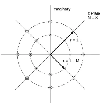
Real N = 8 z Plane Imaginary r = 1 r = 1 – M
Figure 15. Pole-Zero Placement in z Plane
The zeros must have constant amplitude (|z| = 1) and be equally spaced (2π / N) on the unit circle of the z-plane to create nulls in the frequency response at frequencies kω0. The poles have the same angle (frequency) as the zeros but are equally spaced on the circle at distance (1 – µ) from the origin. The effect of the poles is to introduce a resonance in the vicinity for the null, reducing the bandwidth of the notch. If
µ << 1 is used, the 3-dB bandwidth of each notch can be shown to be:
BW[pTm (Hz) (51)
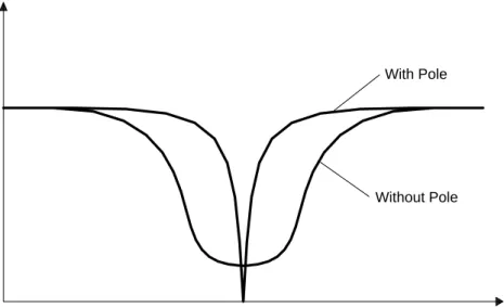
Therefore, the smaller the step size µ, the closer the poles are to the zeros and the narrower the bandwidths of the notches that can be achieved. This effect of a pole on notch bandwidth is shown in Figure 16.
With Pole Without Pole Frequency M agn it u d e
Figure 16. Effect of Pole on Notch Bandwidth Adaptive Notch Filters
The second type of reference signal used in the narrowband ANC system is a sine wave with the same frequency as the narrowband noise to be canceled. When a sine wave is employed as the reference input, the LMS algorithm becomes an adaptive notch filter to remove the primary spectral components within a narrow band centered about the reference frequency. A very narrow notch is usually desired to filter out the interference without distorting the signal and can be realized by an adaptive noise canceler. The advantages of the adaptive notch filter are that it offers easy control of bandwidth, an infinite null, and the capability of adaptively tracking the exact frequency of the interference. This is especially true when the frequency of the interfering sinusoid changes slowly.
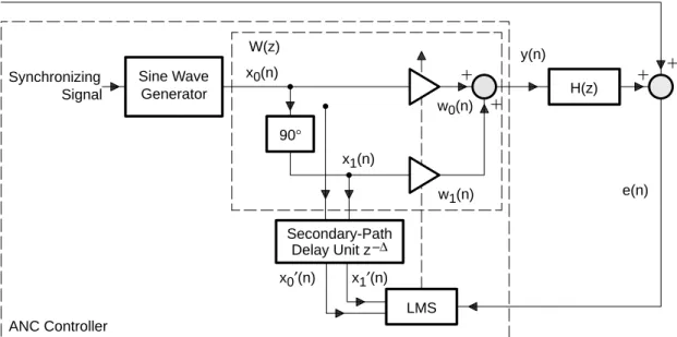
The application of the adaptive notch filter to active periodic noise control was developed by Ziegler [22]. A block diagram of this narrowband ANC system with two adaptive weights is shown in Figure 17. The timing signal sensor, such as an engine tachometer, is used to determine the fundamental frequency at which the repetitive noise is being generated. For example, an electric motor running at 1800 RPM completes 30 revolutions per second with a fundamental frequency of 30 Hz. A four-cylinder engine running at 1800 RPM also completes 30 revolutions per second but with only 15 complete firing cycles per second, and thus has a fundamental frequency 15 Hz.
d(n) Signal Synchronizing H(z) LMS x1(n) w1(n) e(n) y(n) w0(n) x0(n) 90° Secondary-Path Delay Unit z–∆ Generator Sine Wave x1′(n) x0′(n) ANC Controller W(z)
Figure 17. Single-Tone ANC System With Adaptive Notch Filter
The single-frequency active noise controller shown in Figure 17 can be configured in parallel or cascade structures [23] to cancel the narrowband noise at the fundamental frequency and its harmonics. A sine wave generator provides a sinusoidal reference signal at the desired frequency. Employing a Hilbert transform [24] as the 90° phase shifter, the sine wave is split into two orthogonal components, x0(n) and
x1(n), which can be used as reference inputs for the adaptive filter. These two signals are separately
weighted and then summed to produce the canceling signal y(n):
y(n)+ w0(n) x0(n)) w1(n) x1(n) (52) where x0(n)+ A cos(kw0n) (53) and (54) x1(n)+ A sin(kw0n)
where ω0 is the fundamental frequency, k is the harmonic index, A is the amplitude of the reference signal, and n is the time index. The sine-wave generator can be implemented by a ROM table look-up technique or by a digital resonator [24]. Algorithms of a sine-wave generator using both the table look-up and the digital oscillator are given in Appendix B, Digital Sine-Wave Generator.
The magnitude and the phase of this reference signal are adjusted in the controller, which feeds one or more loudspeakers serving as the control source to cancel the corresponding noise components. The LMS algorithm updates the filter weights to minimize the residual error e(n):
w0(n) 1) + w0(n) – me(n) x0(n – Dk) (55)
and
(56) w1(n) 1) + w1(n) – me(n) x1(n – Dk)
where ∆k is used to compensate for the effects of the secondary path at harmonic k. This delay represents the delay introduced between the adaptive filter output and the residual error input.
When the system time delay is fixed, the values can be estimated by an off-line secondary-path modeling technique (described previously; see page 18) and then built into the controller. In general, the values of the delay depend on the frequency. These delays can be determined by converting the impulse response of C(z) into the frequency domain by the discrete Fourier transform and then by calculating the delays from the phase values. That is:
tf+
–Ff
2pf (57)
where tf is the time delay at frequency f in seconds, Ff is the phase at frequency f in radians, and f is the frequency in Hz. The values of ∆k in equations (55) and (56) are then determined by:
Dk+ tf fs (58)
where fs is the sampling rate.
As mentioned previously, the secondary-path delay unit z–∆ in Figure 17 can be replaced by the estimate of the secondary path. The adaptive notch filter algorithm using the FXLMS algorithm can be expressed as:
wi(n) 1) + wi(n) – me(n)xiȀ(n) (59)
Structure for Multiple Frequency Cancellation
In practical applications, the periodic noise usually contains tones at the fundamental frequency and several harmonic frequencies. This type of noise can be attenuated by a filter with multiple notches. In general, realization of multiple notches requires a filter with higher order, which also can be realized by a parallel or cascade connection of multiple second-order sections. A method for eliminating multiple sinusoidals or other periodic interference was proposed by Glover [25]. The application of this technique to active periodic noise control is to generate the reference input as a sum of M sinusoids. That is:
x(n)+
ȍ
M m+1
Amcos(wmn) (60)
where Am and ωm are the amplitude and the frequency of the mth sinusoid, respectively.
When a sum of sinusoids is applied to an adaptive filter, the filter converges to a time-varying, tunable notch filter with a notch located at each of the reference frequencies. As long as a reference is available that includes every sinusoidal interference, the narrowband ANC system creates a notch over each sinusoid and follows it if it changes in frequency. This adaptive notch filter provides a simple method for the tracking and elimination of sinusoidal interferences. The application of Glover’s method for actively attenuating engine-generated noise was patented by Pfaff [26]. The reference signal representing the selected multiple harmonic noise components is generated from a predetermined table of values.
A single-frequency sinusoid can be canceled by the simple 2-weight adaptive filter. For the case where the undesired primary noise contains M sinusoids, M 2-weight adaptive filters can be connected in parallel to attenuate these narrowband components. A set of closely spaced reference sinusoids is synthesized from the information provided by the synchronization signal. A specific sinusoid is used as the reference input for the corresponding channel of the 2-weight adaptive filter Wm(z), which is connected in parallel with
the other filters, as shown in Figure 18.
The structure of each individual channel is shown in Figure 17. The overall transfer function of this parallel configuration is: (61) W(z)+
ȍ
M m+1 Wm(z)where m + 1, 2, … and M is the channel index. The canceling signal is a sum of M adaptive filter outputs. That is: (62) y(n)+
ȍ
M m+1 wm(n)Each reference input is filtered by the secondary-path estimate C(z) as:
(63) xm(n)+
ȍ
L – 1 i+0
cixm(n – 1), m+ 1, 2, AAA , M
Because only one error microphone is used, there is only one error signal e(n) used to update M adaptive filters based on the FXLMS algorithm.
e(n) d(n) xM(n) WM(z) yM(n) y(n) H(z) y1(n) W1(z) x1(n) x0(n) y0(n) W0(z) Sine Wave Generator . . .
Figure 18. Multiple 2-Weight Adaptive Filters in Parallel
Algorithms for Feedback ANC Systems
The principle of feedback ANC for a single-channel case, which can be formulated as an adaptive predictor, is shown in Figure 19. Because this system requires only one error microphone, it avoids the acoustic feedback problem inherent in the 2-microphone feedforward systems that were discussed previously. Feedback ANC schemes depend on the signal having a periodic characteristic. Several nonadaptive feedback ANC systems have been described in the literature in recent years, as reviewed in Nelson’s book [1].
Burgess [3] suggests the use of this configuration with the FXLMS algorithm to avoid the use of the input microphone. The basic idea of this algorithm is to estimate the primary noise d(n) and to use this as the reference input for the adaptive filter. As shown in Figure 19 and using the FXLMS algorithm, the primary noise is estimated as:
(64) x(n) + e(n) –
ȍ
M – 1 i+ 0
ciy (n – i)
where ci (i + 0, 1, … M – 1) is the coefficient of the secondary-path estimation filter C(z) and M is the order of the filter C(z).
x(n) y(n) d(n) H(z) W(z) P(z) C(z) x′(n) e(n) C(z) LMS ANC Controller
Figure 19. Block Diagram of the Feedback ANC System From Figure 19:
(65) D(z)+ E(z) – H(z)Y(z)
where both E(z) and Y(z) are available. If the transfer function H(z) of the secondary path is modeled by C(z):
(66) D(z)[ X(z) + E(z) – C(z)Y(z)
The error signal can be shown as:
(67) E(z)+ D(z) – W(z)H(z)X(z)
The error signal for this feedback ANC system is 0 when:
(68) W(z) H(z) X(z)+ D(z)
which is possible if the primary noise D(z) is periodic and the transfer function W(z)H(z) is equal to a delay equivalent to a multiple of the signal period.