Digital Object Identifier 10.1109/MSP.2013.2297439 Date of publication: 12 February 2015
T
he widespread use of multisensor technology and the emergence of big data sets have highlighted the limitations of standard flat-view matrix models and the necessity to move toward more versatile data analysis tools. We show that higher-order tensors (i.e., multiway arrays) enable such a fundamental para-digm shift toward models that are essentially polynomial, the uniqueness of which, unlike the matrix methods, is guaranteed under very mild and natural conditions. Benefiting from the power of multilinear algebra as their mathematical backbone, data analysis techniques using tensor decompositions are shown to have great flexibility in the choice of constraints which match data properties and extract more general latent compo-nents in the data than matrix-based methods.A comprehensive introduction to tensor decompositions is provided from a signal process-ing perspective, startprocess-ing from the algebraic foundations, via basic canonical polyadic and Tucker models, to advanced cause-effect and multiview data analysis schemes. We show that tensor decompositions enable natural generalizations of some commonly used signal processing para-digms, such as canonical correlation and subspace techniques, signal separation, linear regres-sion, feature extraction, and classification. We also cover computational aspects and point out how ideas from compressed sensing (CS) and scientific computing may be used for addressing the otherwise unmanageable storage and manipulation issues associated with big data sets. The
image licensed by graphic stock
[
Andrzej Cichocki, Danilo P. Mandic,
Anh huy Phan, Cesar F. Caiafa,
Guoxu Zhou, Qibin Zhao, and
Lieven De Lathauwer
]
[
From two-way to multiway component analysis
]
Tensor
DecomposiTions
for Signal Processing
Applications
concepts are supported by illustrative real-world case studies that highlight the benefits of the tensor framework as efficient and promising tools, inter alia, for modern signal processing, data ana-lysis, and machine-learning applications; moreover, these benefits also extend to vector/matrix data through tensorization.
HISTORICAL NOTES
The roots of multiway analysis can be traced back to studies of homogeneous polynomials in the 19th century, with contributors including Gauss, Kronecker, Cayley, Weyl, and Hilbert. In the modern-day interpretation, these are fully symmetric tensors. Decompositions of nonsymmetric tensors have been studied since the early 20th century [1], whereas the benefits of using more than two matrices in factor analysis (FA) [2] have been apparent in several communities since the 1960s. The Tucker decomposition (TKD) for tensors was introduced in psychometrics [3], [4], while the canonical polyadic decomposition (CPD) was independently rediscovered and put into an application context under the names of canonical decomposition (CANDECOMP) in psychometrics [5] and parallel factor model (PARAFAC) in linguistics [6]. Tensors were subsequently adopted in diverse branches of data analysis such as chemometrics, the food industry, and social sciences [7], [8]. When it comes to signal processing, the early 1990s saw a considerable interest in higher-order statistics (HOS) [9], and it was soon realized that, for multivariate cases, HOS are effectively higher-order tensors; indeed, algebraic approaches to independent component analysis (ICA) using HOS [10]–[12] were inherently tensor based. Around 2000, it was realized that the TKD repre-sents a multilinear singular value decomposition (MLSVD) [15]. Generalizing the matrix singular value decomposition (SVD), the workhorse of numerical linear algebra, the MLSVD spurred the interest in tensors in applied mathematics and scientific comput-ing in very high dimensions [16]–[18]. In parallel, CPD was suc-cessfully adopted as a tool for sensor array processing and deterministic signal separation in wireless communication [19], [20]. Subsequently, tensors have been used in audio, image and video processing, machine learning, and biomedical applications, to name but a few areas. The significant interest in tensors and their quickly emerging applications is reflected in books [7], [8],
[12], [21]–[23] and tutorial papers [24]–[31] covering various aspects of multiway analysis.
FROM A MATRIX TO A TENSOR
Approaches to two-way (matrix) component analysis are well estab-lished and include principal component analysis (PCA), ICA, non-negative matrix factorization (NMF), and sparse component analysis (SCA) [12], [21], [32]. These techniques have become standard tools for, e.g., blind source separation (BSS), feature extraction, or classifi-cation. On the other hand, large classes of data arising from modern heterogeneous sensor modalities have a multiway character and are, therefore, naturally represented by multiway arrays or tensors (see the section “Tensorization—Blessing of Dimensionality”).
Early multiway data analysis approaches reformatted the data tensor as a matrix and resorted to methods developed for classical two-way analysis. However, such a flattened view of the world and the rigid assumptions inherent in two-way analysis are not always a good match for multiway data. It is only through higher-order ten-sor decomposition that we have the opportunity to develop sophis-ticated models capturing multiple interactions and couplings instead of standard pairwise interactions. In other words, we can only discover hidden components within multiway data if the ana-lysis tools account for the intrinsic multidimensional patterns pre-sent, motivating the development of multilinear techniques.
In this article, we emphasize that tensor decompositions are not just matrix factorizations with additional subscripts, multi-linear algebra is much more structurally rich than multi-linear alge-bra. For example, even basic notions such as rank have a more subtle meaning, the uniqueness conditions of higher-order ten-sor decompositions are more relaxed and accommodating than those for matrices [33], [34], while matrices and tensors also have completely different geometric properties [22]. This boils down to matrices representing linear transformations and quad-ratic forms, while tensors are connected with multilinear map-pings and multivariate polynomials [31].
NOTATIONS AND CONVENTIONS
A tensor can be thought of as a multi-index numerical array, whereby the order of a tensor is the number of its modes or
[TABLE 1]BASIC NOTATION.
, ,Aa,a
A tenSor, mAtrix, vector, ScAlAr
[ , , , ]a a a
A= 1 2f R mAtrix A with column vectorS ar
(:, , , , )i i i
a 2 3f N Fiber oF tenSor A obtAined by Fixing All but one index
(:,:, , , )i i
A 3f N mAtrix Slice oF tenSor A obtAined by Fixing All but two indiceS
(:,:,:, , , )i i
A 4f N tenSor Slice oF A obtAined by Fixing Some indiceS
( , , , )
A I I1 2fIN SubtenSor oF A obtAined by reStricting indiceS to belong to SubSetS { , , , }1 2 I
In3 f n
A( )n!RIn#I I1 2gIn-1In+1gIN mode-n mAtricizAtion oF tenSor A!RI1# #I2 g#IN whoSe entry At row i
n And column (i1-1)I2gIn-1In+1gIN+g+(iN-1-1)IN+iN iS equAl to ai i12fiN
A
vec^ h!RI IN N-1gI1 vectorizAtion oF tenSor A!RI1# #I2g#IN with the entry At PoSition
[( ) ]
i1+
/
kN=2 ik-1I I1 2gIk-1 equAl to ai i12fNi ( , , , )diag
D= m m1 2fmR diAgonAl mAtrix with drr=mr
( , , , ) diag
D= N m m1 2fmR diAgonAl tenSor oF order N with drr rg=mr
,
dimensions; these may include space, time, frequency, trials, classes, and dictionaries. A real-valued tensor of order N is denoted by A!RI1#I2#g#IN and its entries by a .
, , ,
i i1 2fiN Then, an N 1#
vector a is considered a tensor of order one, and an N M# matrix
A a tensor of order two. Subtensors are parts of the original data tensor, created when only a fixed subset of indices is used. Vector-valued subtensors are called fibers, defined by fixing every index but one, and matrix-valued subtensors are called slices, obtained by fix-ing all but two indices (see Table 1). The manipulation of tensors often requires their reformatting (reshaping); a particular case of reshaping tensors to matrices is termed matrix unfolding or
matri-cization (see Figure 1). Note that a mode- n multiplication of a
ten-sor A with a matrix B amounts to the multiplication of all mode-n vector fibers with ,B and that, in linear algebra, the ten-sor (or outer) product appears in the expression for a rank-1 mat-rix: abT=a b.
%
Basic tensor notations are summarized in Table 1, various product rules used in this article are given in Table 2, while Figure 2 shows two particular ways to construct a tensor.INTERPRETABLE COMPONENTS IN TWO-WAY DATA ANALYSIS
The aim of BSS, FA, and latent variable analysis is to decompose a data matrix X!RI J# into the factor matrices A [ ,a
1 = , , ] a2f aR !RI R# and B=[ , , , ]b b1 2f bR !RJ R# as X ADBT E a b E r r R r rT 1 m = + = + =
/
, E a b r r R r r 1 % m = + =/
(1)where D= ( , , , )diag m m1 2fmR is a scaling (normalizing) matrix,
the columns of B represent the unknown source signals (factors or latent variables depending on the tasks in hand), the columns of A
represent the associated mixing vectors (or factor loadings), while
E is noise due to an unmodeled data part or model error. In other words, model (1) assumes that the data matrix X comprises hidden components br ^r=1 2, , ,f Rh that are mixed together in an
unknown manner through coefficients A, or, equivalently, that data contain factors that have an associated loading for every data chan-nel. Figure 3(a) depicts the model (1) as a dyadic decomposition, whereby the terms a br
%
r=a br rT are rank-1 matrices.The well-known indeterminacies intrinsic to this model are: 1) arbitrary scaling of components and 2) permutation of the rank-1 terms. Another indeterminacy is related to the physical meaning of the factors: if the model in (1) is unconstrained, it admits infinitely many combinations of A and .B Standard matrix factorizations in linear algebra, such as QR-factorization, eigenvalue decomposition (EVD), and SVD, are only special
... ... ... I J K I X(3) X(2) U1 (SVD/PCA) VT 1 X(:, :, k) K I I X(1) J J X(:, j, :) A2 (NMF/SCA) BT J K K A3 (ICA) BT = S 3 X(i, :, :) Σ = ~ = ~ = ~ 2 (a) (b) (c) Unfolding
[FIg1] MWCA for a third-order tensor, assuming that the components are (a) principal and orthogonal in the first mode, (b) nonnegative and sparse in the second mode, and (c) statistically independent in the third mode.
[TABLE 2] DEFINITION OF PRODuCTS.
B
C=A#n mode-n Product oF A!RI1# #I2 g#IN And B!RJn#In yieldS C!RI1#g#In-1#Jn#In+1#g#IN with entrieS ci in j in n iN iIn 1ai in i in n iNbj in n
n
1g-1 +1g =
/
= 1g-1 +1g And mAtrix rePreSentAtion C( )n=BA( )n;B B, , ,B
C= "A ( )1 ( )2f ( )N, Full multilineAr Product, C A B( ) B( ) B( )
N N
1 1 2 2 # # g# =
C=A B
%
tenSor or outer Product oF A!RI1# #I2 g#IN And B!RJ1#J2#g#JM yieldS C!RI1# #I2g#IN#J1#J2#g#JM withentrieS ci i1 2gi j jN1 2gjM=ai i1 2giNbj j1 2gjM a a a
X= ( )1
%
( )2% %
g ( )N tenSor or outer Product oF vectorS a( )n!RIn (n=1, , )fN yieldS A rAnk-1 tenSor X!RI1# #I2 g#INwith entrieS x a a( ) ( ) a( )
i i1 2fiN= i11 i22f iNN
C=A B7 kronecker Product oF A!RI1#I2 And B!RJ1#J2 yieldS C!RI J1 1#I J2 2 with entrieS
c(i1-1)J1+j i1,(2-1)J2+j2=ai i1 2bj j1 2
C=A B9 khAtri–rAo Product oF A=[ , , ]a1faR !RI R# And B=[ , , ]b1fbR!RJ R# yieldS C!RIJ R# with columnS
cases of (1), and owe their uniqueness to hard and restrictive constraints such as triangularity and orthogonality. On the other hand, certain properties of the factors in (1) can be repre-sented by appropriate constraints, making possible the unique estimation or extraction of such factors. These constraints include statistical independence, sparsity, nonnegativity, expo-nential structure, uncorrelatedness, constant modulus, finite alphabet, smoothness, and unimodality. Indeed, the first four properties form the basis of ICA [12]–[14], SCA [32], NMF [21], and harmonic retrieval [35].
TENSORIZATION—BLESSINg OF DIMENSIONALITY While one-way (vectors) and two-way (matrices) algebraic struc-tures were, respectively, introduced as natural representations for segments of scalar measurements and measurements on a grid, tensors were initially used purely for the mathematical benefits they provide in data analysis; for instance, it seemed natural to stack together excitation–emission spectroscopy matrices in chemometrics into a third-order tensor [7].
The procedure of creating a data tensor from lower-dimen-sional original data is referred to as tensorization, and we propose the following taxonomy for tensor generation:
1) Rearrangement of lower-dimensional data structures: Large-scale vectors or matrices are readily tensorized to higher-order tensors and can be compressed through tensor decompositions if they admit a low-rank tensor approxima-tion; this principle facilitates big data analysis [23], [29], [30] [see Figure 2(a)]. For instance, a one-way exponential signal
( )
x k =azk can be rearranged into a rank-1 Hankel matrix or
a Hankel tensor [36] ( ) ( ) ( ) ( ) ( ) ( ) ( ) ( ) ( ) , H b b x x x x x x x x x a 0 1 2 1 2 3 2 3 4 h h h g g g = =
%
J L K K K KK N P O O O OO (2)where b=[ , , , ]1 z z2 fT. Also, in sensor array processing, tensor structures naturally emerge when combining snap-shots from identical subarrays [19].
2) Mathematical construction: Among many such examples, the Nth-order moments (cumulants) of a vector-valued random variable form an Nth-order tensor [9], while in second-order ICA, snapshots of data statistics (covariance matrices) are effect-ively slices of a third-order tensor [12], [37]. Also, a (channel#
time) data matrix can be transformed into a (channel#time#
frequency) or (channel#time#scale) tensor via time-frequency or wavelet representations, a powerful procedure in multi-channel electroencephalogram (EEG) analysis in brain sci-ence [21], [38].
3) Experiment design: Multifaceted data can be naturally stacked into a tensor; for instance, in wireless communica-tions the so-called signal diversity (temporal, spatial, spec-tral, etc.) corresponds to the order of the tensor [20]. In the same spirit, the standard eigenfaces can be generalized to tensor faces by combining images with different illumina-tions, poses, and expressions [39], while the common modes in EEG recordings across subjects, trials, and conditions are best analyzed when combined together into a tensor [28]. 4) Natural tensor data: Some data sources are readily gen-erated as tensors [e.g., RGB color images, videos, three-dimensional (3-D) light field displays] [40]. Also, in scientific computing, we often need to evaluate a discretized multivariate function; this is a natural tensor, as illustrated in Figure 2(b) for a trivariate function ( , , )f x y z [23], [29], [30].
The high dimensionality of the tensor format is therefore associated with blessings, which include the possibilities to obtain compact representations, the uniqueness of decompositions, the flexibility in the choice of constraints, and the generality of com-ponents that can be identified.
CANONICAL POLYADIC DECOMPOSITION DEFINITION
A polyadic decomposition (PD) represents an Nth-order tensor R
X! I1# #I2 g#IN as a linear combination of rank-1 tensors in the form . b b b X ( ) ( ) ( ) r r R r r rN 1 1 2 g m = =
%
%
%
/
(3)Equivalently, X is expressed as a multilinear product with a diagonal core B B B X D ( ) ( ) ( ) N N 1 1 2 2 # # g# = , ;B B, , ,B D ( )1 ( )2 f ( )N =" , (4)
where D= ( , , , )diagN m m1 2fmR [cf. the matrix case in (1)].
Figure 3 illustrates these two interpretations for a third-order I = 26 (64 × 1)(8 × 8) + ··· + (2 × 2 × 2 × 2 × 2 × 2) z0 z0 + ∆z z0 + 2∆z y0 y0 + ∆y y0 + 2∆y x0 + ∆ x x0 + 2∆ x x0 z x y (a) (b)
[FIg2] Construction of tensors. (a) The tensorization of a vector or matrix into the so-called quantized format; in scientific computing, this facilitates supercompression of large-scale vectors or matrices. (b) The tensor is formed through the discretization of a trivariate function ( , , ).f x y z
tensor. The tensor rank is defined as the smallest value of R for which (3) holds exactly; the minimum rank PD is called
canoni-cal PD (CPD) and is desired in signal separation. The term CPD
may also be considered as an abbreviation of CANDECOMP/ PARAFAC decomposition, see the “Historical Notes” section. The matrix/vector form of CPD can be obtained via the Khatri–Rao products (see Table 2) as
, X( )n =B D B( )n ^ ( )N9g9B(n+1)9B(n-1)9g9B( )1hT ( ) [B B B ] ,d vec X = ( )N 9 (N 1-)9g9 ( )1 (5) where d=[m m1, , ,2fmR]T. RANK
As mentioned earlier, the rank-related properties are very different for matrices and tensors. For instance, the number of complex-valued rank-1 terms needed to represent a higher-order tensor can be strictly smaller than the number of real-valued rank-1 terms [22], while the determination of tensor rank is in gen-eral NP-hard [41]. Fortunately, in signal processing applications, rank estimation most often corresponds to determining the num-ber of tensor components that can be retrieved with sufficient accuracy, and often there are only a few data components present. A pragmatic first assessment of the number of components may be through inspection of the multilinear singular value spectrum (see the “Tucker Decomposition” section), which indicates the size of the core tensor in the right-hand side of Figure 3(b). The existing techniques for rank estimation include the core consistency diag-nostic (CORCONDIA) algorithm, which checks whether the core tensor is (approximately) diagonalizable [7], while a number of techniques operate by balancing the approximation error versus the number of degrees of freedom for a varying number of rank-1 terms [42]–[44].
UNIQUENESS
Uniqueness conditions give theoretical bounds for exact tensor decompositions. A classical uniqueness condition is due to Kruskal [33], which states that for third-order tensors, the CPD is unique up to unavoidable scaling and permutation ambiguities, provided that
,
kB( )1+kB( )2+kB( )3$2R+2 where the Kruskal rank kB of a matrix
B is the maximum value ensuring that any subset of kB columns is linearly independent. In sparse modeling, the term (kB+1) is also known as the spark [32]. A generalization to Nth-order tensors is due to Sidiropoulos and Bro [45] and is given by
. k 2R N 1 n N 1 B( )n $ + -=
/
(6)More relaxed uniqueness conditions can be obtained when one factor matrix has full-column rank [46]–[48]; for a thorough study of the third-order case, we refer to [34]. This all shows that, compared to matrix decompositions, CPD is unique under more natural and relaxed conditions, which only require the compo-nents to be sufficiently different and their number not unreason-ably large. These conditions do not have a matrix counterpart and are at the heart of tensor-based signal separation.
COMPUTATION
Certain conditions, including Kruskal’s, enable explicit computa-tion of the factor matrices in (3) using linear algebra [essentially, by solving sets of linear equations and computing (generalized) EVD] [6], [47], [49], [50]. The presence of noise in data means that CPD is rarely exact, and we need to fit a CPD model to the data by minimizing a suitable cost function. This is typically achieved by minimizing the Frobenius norm of the difference between the given data tensor and its CP approximation, or, alter-natively, by least absolute error fitting when the noise is Lapla-cian [51]. The theoretical Cramér–Rao lower bound and
X br br ar a1 aR bR b1 + ··· + (I × J ) λ1 λR (R × J ) (R × R ) (I × R ) = = ∼ = ∼ A D (a) cr ar a1 b1 c1 + ··· + (I × J × k ) λR bR cR (K × R ) (R × J ) (R × R× R ) (I × R ) aR λ1 A
=
BT BT C (b)[FIg3] The analogy between (a) dyadic decompositions and (b) PDs; the Tucker format has a diagonal core. The uniqueness of these decompositions is a prerequisite for BSS and latent variable analysis.
Cramér–Rao induced bound for the assessment of CPD perform-ance were derived in [52] and [53].
Since the computation of CPD is intrinsically multilinear, we can arrive at the solution through a sequence of linear subprob-lems as in the alternating least squares (ALS) framework, whereby the least squares (LS) cost function is optimized for one component matrix at a time, while keeping the other com-ponent matrices fixed [6]. As seen from (5), such a conditional update scheme boils down to solving overdetermined sets of linear equations.
While the ALS is attractive for its simplicity and satisfactory performance for a few well-separated components and at suffi-ciently high signal-to-noise ratio (SNR), it also inherits the problems of alternating algorithms and is not guaranteed to converge to a stationary point. This can be rectified by only updating the factor matrix for which the cost function has most decreased at a given step [54], but this results in an N-times increase in computational cost per iteration. The convergence of ALS is not yet completely understood—it is quasilinear close to the stationary point [55], while it becomes rather slow for ill-conditioned cases; for more details, we refer to [56] and [57].
The conventional all-at-once algorithms for numerical optimi-zation, such as nonlinear conjugate gradients, quasi-Newton, or nonlinear least squares (NLS) [58], [59], have been shown to often outperform ALS for ill-conditioned cases and to be typically more robust to overfactoring. However, these come at the cost of a much higher computational load per iteration. More sophisticated ver-sions use the rank-1 structure of the terms within CPD to perform efficient computation and storage of the Jacobian and (approxi-mate) Hessian; their complexity is on par with ALS while, for ill-conditioned cases, the performance is often superior [60], [61].
An important difference between matrices and tensors is that the existence of a best rank- R approximation of a tensor of rank greater than R is not guaranteed [22], [62] since the set of ten-sors whose rank is at most R is not closed. As a result, the cost functions for computing factor matrices may only have an infi-mum (instead of a miniinfi-mum) so that their minimization will approach the boundary of that set without ever reaching the boundary point. This will cause two or more rank-1 terms go to infinity upon convergence of an algorithm; however, numerically, the diverging terms will almost completely cancel one another while the overall cost function will still decrease along the itera-tions [63]. These diverging terms indicate an inappropriate data model: the mismatch between the CPD and the original data ten-sor may arise because of an underestimated number of compo-nents, not all tensor components having a rank-1 structure, or data being too noisy.
CONSTRAINTS
As mentioned earlier, under quite mild conditions, the CPD is unique by itself, without requiring additional constraints. However, to enhance the accuracy and robustness with respect to noise, prior knowledge of data properties (e.g., statistical independence, spars-ity) may be incorporated into the constraints on factors so as to facilitate their physical interpretation, relax the uniqueness
conditions, and even simplify computation [64]–[66]. Moreover, the orthogonality and nonnegativity constraints ensure the existence of the minimum of the optimization criterion used [63], [64], [67]. APPLICATIONS
The CPD has already been established as an advanced tool for sig-nal separation in vastly diverse branches of sigsig-nal processing and data analysis, such as in audio and speech processing, biomedical engineering, chemometrics, and machine learning [7], [24], [25], [28]. Note that algebraic ICA algorithms are effectively based on the CPD of a tensor of the statistics of recordings; the statistical independence of the sources is reflected in the diagonality of the core tensor in Figure 3, i.e., in vanishing cross-statistics [11], [12]. The CPD is also heavily used in exploratory data analysis, where the rank-1 terms capture the essential properties of dynamically complex signals [8]. Another example is in wireless communica-tion, where the signals transmitted by different users correspond to rank-1 terms in the case of line-of-sight propagation [19]. Also, in harmonic retrieval and direction of arrival type applications, real or complex exponentials have a rank-1 structure, for which the use of CPD is natural [36], [65].
EXAMPLE 1
Consider a sensor array consisting of K displaced but otherwise identical subarrays of I sensors, with Iu=KI sensors in total. For R narrowband sources in the far field, the baseband equiva-lent model of the array output becomes X=AST+E, where
A!CI Ru# is the global array response, S!CJ R# contains J
snapshots of the sources, and E is the noise. A single source )
(R=1 can be obtained from the best rank-1 approximation of the matrix X; however, for R21, the decomposition of X is not unique, and, hence, the separation of sources is not possible without incorporating additional information. The constraints on the sources that may yield a unique solution are, for instance, constant modulus and statistical independence [12], [68].
Consider a row-selection matrix Jk!CI I#u that extracts the rows of X corresponding to the kth subarray, k=1, , .f K For two identical subarrays, the generalized EVD of the matrices
J X1 and J X2 corresponds to the well-known estimation of
sig-nal parameters via rotatiosig-nal invariance techniques (ESPRIT) [69]. For the case K22, we shall consider J Xk as slices of the
tensor X!CI J K# # (see the section “Tensorization—Blessing
of Dimensionality”). It can be shown that the signal part of
X admits a CPD as in (3) and (4), with m1=g=mR=1,
( , , ),
J A B( )diag b( ) b( )
k = 1 k31 f kR3 and B( )2 =S[19], and the
conse-quent source separation under rather mild conditions—its uniqueness does not require constraints such as statistical inde-pendence or constant modulus. Moreover, the decomposition is unique even in cases when the number of sources, ,R exceeds the
number of subarray sensors, ,I or even the total number of sen-sors, .Iu Note that particular array geometries, such as linearly
and uniformly displaced subarrays, can be converted into a con-straint on CPD, yielding a further relaxation of the uniqueness conditions, reduced sensitivity to noise, and often faster computation [65].
TuCKER DECOMPOSITION
Figure 4 illustrates the principle of TKD, which treats a tensor R
X! I1#I2#g#IN as a multilinear transformation of a (typically dense but small) core tensor G!RR1#R2#g#RN by the factor matrices B( )n [b( )n,b( )n, ,b( )] R , Rn I R 1 2 n n n f ! = # n=1 2, , ,f N [3], [4], given by , b b b g X ( ) ( ) ( ) r r r r r rN r R r R r R 1 2 1 1 1 N N N N 1 2 1 2 2 2 1 1
%
% %
g g = g = = = ^ h/
/
/
(7) or equivalently B B B X G ( ) ( ) ( ) N N 1 1 2 2 # # g# = ;GB B( )1, ( )2, ,f B( )N . = " , (8)Via the Kronecker products (see Table 2), TKD can be expressed in a matrix/vector form as ( ) X( )n =B G( )n ( )n B( )N7g7B(n+1)7B(n-1)7g7B( )1 T . ( ) [B B B ] ( ) vec X = ( )N7 (N 1-)7g7 ( )1 vec G
Although Tucker initially used the orthogonality and ordering constraints on the core tensor and factor matrices [3], [4], we can also employ other meaningful constraints.
MULTILINEAR RANK
For a core tensor of minimal size, R1 is the column rank (the
dimension of the subspace spanned by mode-1 fibers), R2 is the
row rank (the dimension of the subspace spanned by mode-2 fibers), and so on. A remarkable difference from matrices is that the values of ,R R1 2, ,f RN can be different for N$3. The N-tuple ( ,R R1 2, ,f RN) is consequently called the multilinear
rank of the tensor X.
LINKS BETWEEN CPD AND TUCKER DECOMPOSTION TKD can be considered an expansion in rank-1 terms (polyadic but not necessary canonical), as shown in (7), while (4) represents CPD as a multilinear product of a core tensor and factor matrices (but the core is not necessary minimal); Table 3 shows various other connections. However, despite the obvious interchangeabil-ity of notation, the CPD and TKD serve different purposes. In gen-eral, the Tucker core cannot be diagonalized, while the number of CPD terms may not be bounded by the multilinear rank. Conse-quently, in signal processing and data analysis, CPD is typically used for factorizing data into easy to interpret components (i.e., the rank-1 terms), while the goal of unconstrained TKD is most often to compress data into a tensor of smaller size (i.e., the core tensor) or to find the subspaces spanned by the fibers (i.e., the col-umn spaces of the factor matrices).
UNIQUENESS
The unconstrained TKD is in general not unique, i.e., factor matri-ces B( )n are rotation invariant. However, physically, the subspaces
defined by the factor matrices in TKD are unique, while the bases in these subspaces may be chosen arbitrarily—their choice is compensated for within the core tensor. This becomes clear upon
realizing that any factor matrix in (8) can be postmultiplied by any nonsingular (rotation) matrix; in turn, this multiplies the core tensor by its inverse, i.e.,
;B B, , ,B X= "G ( )1 ( )2 f ( )N, ,H;B R B R( )1 ( )1, ( )2 ( )2, ,f B R( )N ( )N = " , , ;R ,R , ,R H G ( )1 1 ( )2 1 ( )N 1 f = " - - -, (9)
where the matrices R( )n are invertible.
MULTILINEAR SVD
Orthonormal bases in a constrained Tucker representation can be obtained via the SVD of the mode- n matricized tensor
X( )n =UnRn nVT (i.e., B( )n =Un, n=1 2, , , ).f N Because of the
orthonormality, the corresponding core tensor becomes . U U U S X T T N NT 1 1 2 2 # # g# = (10) C A (I1 × I2 × I3) (R1 × R2 × R3) (R2 × l2) (l3 × R3) (I× R1) BT = ∼
[FIg4] The Tucker decompostion of a third-order tensor. The column spaces of ,A ,B and c represent the signal subspaces for the three modes. The core tensor G is nondiagonal, accounting for the possibly complex interactions among tensor components.
[TABLE 3]DIFFERENT FORMS OF CPD AND TuCKER
REPRESENTATIONS OF A ThIRD-ORDER TENSOR X!RI J K# # .
CPD TKD
tenSor rePreSentAtion, outer ProductS
a b c X r r r r r R 1 % % m = =
/
X gr r rar br cr r R r R r R 1 1 1 1 2 3 1 2 3 3 3 2 2 1 1 % % = = = =/
/
/
tenSor rePreSentAtion, multilineAr ProductS
A B C X=D#1 #2 #3 X=G#1A#2B#3C mAtrix rePreSentAtionS ( ) X( )1=A D C B9 T X( )1=A G C B( )1( 7 )T ( ) X( )2=B D C A9 T X( )2=B G C A( )2( 7 )T ( ) X( )3=C D B A9 T X( )3=C G B A( )3( 7 )T vector rePreSentAtion ( ) (C B A)d
vecX = 9 9 vec( )X =(C B A7 7 )vec( )G
ScAlAr rePreSentAtion xijk ra b cir jr kr r R 1 m = =
/
xijk gr r ra b cir jr kr r R r R r R 1 1 1 1 2 3 1 2 3 3 3 2 2 1 1 = = = =/
/
/
mAtrix SliceS Xk=X(:,:, )k ( ,c c , ,c ) diag Xk=A k1 k2f kRBT (:,:, ) c r Xk A kr G B r R T 1 3 3 3 3 = =/
Then, the singular values of X( )n are the Frobenius norms of
the corresponding slices of the core tensor :S ( )Rn r rn n, =
(:, :, , , :, ,:) ,r
S f n f F with slices in the same mode being
mutually orthogonal, i.e., their inner products are zero. The col-umns of Un may thus be seen as multilinear singular vectors, while the norms of the slices of the core are multilinear singular values [15]. As in the matrix case, the multilinear singular values govern the multilinear rank, while the multilinear singular vectors allow, for each mode separately, an interpretation as in PCA [8]. LOW MULTILINEAR RANK APPROXIMATION
Analogous to PCA, a large-scale data tensor X can be approxi-mated by discarding the multilinear singular vectors and slices of the core tensor that correspond to small multilinear singular val-ues, i.e., through truncated matrix SVDs. Low multilinear rank approximation is always well posed; however, the truncation is not necessarily optimal in the LS sense, although a good estimate can often be made as the approximation error corresponds to the degree of truncation. When it comes to finding the best approxi-mation, the ALS-type algorithms exhibit similar advantages and drawbacks to those used for CPD [8], [70]. Optimization-based algorithms exploiting second-order information have also been proposed [71], [72].
CONSTRAINTS AND TUCKER-BASED MULTIWAY COMPONENT ANALYSIS
Besides orthogonality, constraints that may help to find unique basis vectors in a Tucker representation include statistical inde-pendence, sparsity, smoothness, and nonnegativity [21], [73], [74]. Components of a data tensor seldom have the same properties in its modes, and for physically meaningful representation, different constraints may be required in different modes so as to match the properties of the data at hand. Figure 1 illustrates the concept of multiway component analysis (MWCA) and its flexibility in choos-ing the modewise constraints; a Tucker representation of MWCA naturally accommodates such diversities in different modes.
OTHER APPLICATIONS
We have shown that TKD may be considered a multilinear extension of PCA [8]; it therefore generalizes signal subspace techniques, with applications including classification, feature extraction, and subspace-based harmonic retrieval [27], [39], [75], [76]. For instance, a low multilinear rank approximation achieved through TKD may yield a higher SNR than the SNR in the original raw data tensor, making TKD a very natural tool for compression and signal enhancement [7], [8], [26].
BLOCK TERM DECOMPOSITIONS
We have already shown that CPD is unique under quite mild con-ditions. A further advantage of tensors over matrices is that it is even possible to relax the rank-1 constraint on the terms, thus opening completely new possibilities in, e.g., BSS. For clarity, we shall consider the third-order case, whereby, by replacing the rank-1 matrices b( ) b( ) b b( ) ( )
r1 % r2 = r1 r2T in (3) by low-rank matrices
,
A Br rT the tensor X can be represented as [Figure 5(a)]
(A B) c . X r R r rT r 1 % = =
/
(11)Figure 5(b) shows that we can even use terms that are only required to have a low multilinear rank (see the “Tucker Decom-position” section) to give
. A B C X Gr r R r r r 1 1 2 3 # # # = =
/
(12)These so-called block term decompositions (BTDs) in (11) and (12) admit the modeling of more complex signal components than CPD and are unique under more restrictive but still fairly natural conditions [77]–[79].
EXAMPLE 2
To compare some standard and tensor approaches for the separa-tion of short durasepara-tion correlated sources, BSS was performed on five linear mixtures of the sources ( )s t1 =sin(6rt) and
( ) exp( )sin( ),
s t2 = 10t 20rt which were contaminated by white
Gaussian noise, to give the mixtures X=AS E+ !R5 60# , where ( ) [ ( ), ( )]
S t s t s t T
1 2
= and A! R5 2# was a random matrix whose
columns (mixing vectors) satisfy a aT 0 1. ,
1 2= a1 2= a2 2=1.
The 3-Hz sine wave did not complete a full period over the 60 sam-ples so that the two sources had a correlation degree of (|s sT |)/( s s ) 0 35. .
1 2 1 2 2 2 = The tensor approaches, CPD, TKD,
and BTD employed a third-order tensor X of size 24 # 37 # 5 generated from five Hankel matrices whose elements obey
( , , )i j k
X =X( ,k i j 1+ - ) (see the section “Tensorization— Blessing of Dimensionality”). The average squared angular error (SAE) was used as the performance measure. Figure 6 shows the simulation results, illustrating the following.
■ PCA failed since the mixing vectors were not orthogonal
and the source signals were correlated, both violating the assumptions for PCA.
■ The ICA [using the joint approximate diagonalization of
eigenmatrices (JADE) algorithm [10]] failed because the sig-nals were not statistically independent, as assumed in ICA.
A1 (I × J × K ) (I × L1) (L1 × J ) BT AR + ··· + (I × LR) (LR × J ) c1 cR (K ) (K ) 1 BRT = ~ (K × N1) (I × J × K ) (I × L1) (M1 × J ) + ··· + C1 CR A1 AR (LR × MR× NR) BT 1 BRT = ~ 1 R (a) (b)
[FIg5] BTDs find data components that are structurally more complex than the rank-1 terms in CPD. (a) Decomposition into terms with multilinear rank ( , , ).L L 1r r (b) Decomposition into terms with multilinear rank ( ,L M Nr r, r).
■ Low-rank tensor approximation via a rank-2 CPD was used
to estimate A as the third factor matrix, which was then inverted to yield the sources. The accuracy of CPD was com-promised as the components of tensor X cannot be repre-sented by rank-1 terms.
■ Low multilinear rank approximation via TKD for the
mul-tilinear rank (4, 4, 2) was able to retrieve the column space of the mixing matrix but could not find the individual mixing vectors because of the nonuniqueness of TKD.
■ BTD in multilinear rank-(2, 2, 1) terms matched the data
structure [78]; it is remarkable that the sources were recov-ered using as few as six samples in the noise-free case. hIghER-ORDER COMPRESSED SENSINg (hO-CS)
The aim of CS is to provide a faithful reconstruction of a signal of interest, even when the set of available measurements is (much) smaller than the size of the original signal [80]–[83]. Formally, we have available M (compressive) data samples y!RM, which are assumed to be linear transformations of the original signal x!RI
(M1I). In other words, y=Ux, where the sensing matrix RM I
!
U # is usually random. Since the projections are of a lower
dimension than the original data, the reconstruction is an ill-posed inverse problem whose solution requires knowledge of the physics
of the problem converted into constraints. For example, a two-dimensional image X!RI1#I2 can be vectorized as a long vector
( )X
x=vec !RI (I I I)
1 2
= that admits sparse representation in a known dictionary B!RI I# so that x=Bg, where the matrix B
may be a wavelet or discrete cosine transform dictionary. Then, faithful recovery of the original signal x requires finding the spars-est vector g such that
, ,
W W B,
y= g with g 0#K =U (13)
where · 0 is the ,0-norm (number of nonzero entries) and
.
K%I
Since the ,0-norm minimization is not practical, alternative
solutions involve iterative refinements of the estimates of vector g
using greedy algorithms such as the orthogonal matching pur-suit (OMP) algorithm, or the ,1-norm minimization algorithms
g 1=
^
/
iI=1 gij [83]. Low coherence of the composite dictionarymatrix W is a prerequisite for a satisfactory recovery of g (and hence )x—we need to choose U and B so that the correlation between the columns of W is minimum [83].
When extending the CS framework to tensor data, we face two obstacles:
■ loss of information, such as spatial and contextual
relation-ships in data, when a tensor X!RI1#I2#g#IN is vectorized.
0.05 0.1 0.15 0.2 −0.3 −0.2 −0.1 0 0.1 Time (s) 0.05 0.1 0.15 0.2 Time (s) 0.05 0.1 0.15 0.2 Time (s) s1 −0.2 −0.1 0 0.1 s1 s ˆsPCA ˆsICA ˆsCPD s ˆsCPD ˆsTKD ˆsBTD s ˆsCPD ˆsTKD ˆsBTD −0.2 −0.1 0 0.1 0.2 0.3 s2 0 10 20 30 40 0 20 40 60 SNR (dB) (a) (b) (c) (d) SAE (dB) PCA ICA CPD TKD BTD
[FIg6] The blind separation of the mixture of a pure sine wave and an exponentially modulated sine wave using PCA, ICA, CPD, TKD, and BTD. The sources s1 and s2 are correlated and of short duration; the symbols st1 and st2 denote the estimated sources. (a)–(c)
Sources ( )s1t and ( )s2 t and their estimates using PCA, ICA, CPD, TKD, and BTD; (d) average squared angular errors (SAE) in estimation
■ data handling since the size of vectorized data and the
associated dictionary B!RI I# easily becomes prohibitively
large (see the section “Large-Scale Data and the Curse of Dimensionality”), especially for tensors of high order.
Fortunately, tensor data are typically highly structured, a per-fect match for compressive sampling, so that the CS framework relaxes data acquisition requirements, enables compact storage, and facilitates data completion (i.e., inpainting of missing samples due to a faulty sensor or unreliable measurement).
KRONECKER-CS FOR FIXED DICTIONARIES
In many applications, the dictionary and the sensing matrix admit a Kronecker structure (Kronecker-CS model), as illustrated in Figure 7(a) [84]. In this way, the global composite dictionary matrix becomes W=W( )N7W(N 1-)7g7W( )1, where each term W( )n =U( )nB( )n has a reduced dimensionality since
B( )n !RIn#In and U( )n !RMn#In. Denote M M M M N 1 2g
= and
,
I=I I1 2gIN then, since Mn#In, n=1 2, , , ,f N this reduces
storage requirements by a factor of (Rn nI Mn)/( ).MI The
compu-tation of Wg is affordable since g is sparse; however, computing
WTy is expensive but can be efficiently implemented through a
sequence of products involving much smaller matrices W( )n [85].
We refer to [84] for links between the coherence of factor matri-ces W( )n and the coherence of the global composite dictionary
matrix .W
Figure 7 and Table 3 illustrate that the Kronecker-CS model is effectively a vectorized TKD with a sparse core. The tensor equivalent of the CS paradigm in (13) is therefore to find the sparsest core tensor G such that
, W W W Y G ( ) ( ) ( ) N N 1 1 2 2 # # g# , (14)
with G 0#K, for a given set of modewise dictionaries B( )n and sensing matrices U( )n(n=1 2, , ,f N). Working with several
small dictionary matrices, appearing in a Tucker representation, instead of a large global dictionary matrix, is an example of the use of tensor structure for efficient representation; see also the section “Large-Scale Data and the Curse of Dimensionality.”
A higher-order extension of the OMP algorithm, referred to as the Kronecker-OMP algorithm [85], requires K iterations to find the K nonzero entries of the core tensor .G Additional computa-tional advantages can be gained if it can be assumed that the K nonzero entries belong to a small subtensor of ,G as shown in Figure 7(b); such a structure is inherent to, e.g., hyperspectral imaging [85], [86] and 3-D astrophysical signals. More precisely, if the K=LN nonzero entries are located within a subtensor of size
(L L# #g#L), where L%In, then, by exploiting the block-tensor structure, the so-called N-way block OMP algorithm (N-BOMP) requires at most NL iterations, which is linear in N W y W(3) W(3) W(2) W(2) W(1) W(1) ⊗ g Sparse Vector Representation (Kronecker-CS) Measurement Vector (CS) Sparse Vector (M1M2M3 × I1I2I3) (M1 × M2 × M3) (M1 × l1) (l1 × l2 × l3) (M2 × l2) (M3 × I3) (I1I2I3) (M1M2M3) Measurement Tensor (CS) Block Sparse Core Tensor
Block Sparse Tucker Representation =
~
= ~
⊗
(a) Vector Representation
(b) Tensor Representation
[FIg7] CS with a Kronecker-structured dictionary. OMP can perform faster if the sparse entries belong to a small subtensor, up to permutation of the columns of W( )1, W( )2, and W( )3.
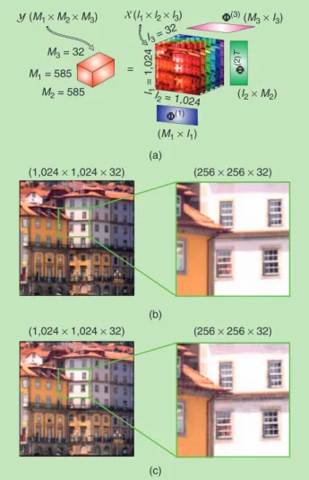
[FIg8] The multidimensional CS of a 3-D hyperspectral image using Tucker representation with a small sparse core in wavelet bases. (a) The Kronecker-CS of a 32-channel hyperspectral image. (b) The original hyperspectral image-RgB display. (c) The reconstruction (SP = 33%, PSNR = 35.51 dB)-RgB display. (a) (b) (c) (1,024 × 1,024 × 32) (256 × 256 × 32) (1,024 × 1,024 × 32) (256 × 256 × 32) = (M1 × M2 × M3) (l1 × l2 × l3) Φ(3) (M3× I3) Φ(1) Φ (2 )T M3 = 32 M1 = 585 M2 = 585 I = 1,0241 I3 = 32 I2 = 1,024 (I2× M2) (M1× I1) 32
[85]. The Kronecker-CS model has been applied in magnetic res-onance imaging, hyperspectral imaging, and in the inpainting of multiway data [86], [84].
APPROACHES WITHOUT FIXED DICTIONARIES
In Kronecker-CS, the modewise dictionaries B( )n !RIn#In can be chosen so as best to represent the physical properties or prior knowledge about the data. They can also be learned from a large ensemble of data tensors, for instance, in an ALS-type fashion [86]. Instead of the total number of sparse entries in the core ten-sor, the size of the core (i.e., the multilinear rank) may be used as a measure for sparsity so as to obtain a low-complexity represen-tation from compressively sampled data [87], [88]. Alternatively, a CPD representation can be used instead of a Tucker representa-tion. Indeed, early work in chemometrics involved excitation– emission data for which part of the entries was unreliable because of scattering; the CPD of the data tensor is then computed by treating such entries as missing [7]. While CS variants of several CPD algorithms exist [59], [89], the oracle properties of tensor-based models are still not as well understood as for their standard models; a notable exception is CPD with sparse factors [90]. EXAMPLE 3
Figure 8 shows an original 3-D (1,024#1,024#32) hyperspectral image ,X which contains scene reflectance measured at 32 differ-ent frequency channels, acquired by a low-noise Peltier-cooled dig-ital camera in the wavelength range of 400–720 nm [91]. Within the Kronecker-CS setting, the tensor of compressive measure-ments Y was obtained by multiplying the frontal slices by random Gaussian sensing matrices U( )1 !RM1#1024 and
R
( )2 ! M2 1024
U # ( ,M M 1 024, )
1 21 in the first and second mode,
respectively, while U( )3 !R32 32# was the identity matrix [see
Figure 8(a)]. We used Daubechies wavelet factor matrices
B( )1 =B( )2 !R1024 1024# and B( )3 !R32 32# , and employed the N-way block tensor N-BOMP to recover the small sparse core tensor
and, subsequently, reconstruct the original 3-D image, as shown in Figure 8(b). For the sampling ratio SP=33% (M1=M2=585) this gave the peak SNR (PSNR) of 35.51 dB, while taking 71 min for Niter=841 iterations needed to detect the subtensor which contains the most significant entries. For the same quality of reconstruction (PSNR=35.51 dB), the more conventional Kronecker-OMP algorithm found 0.1% of the wavelet coefficients as significant, thus requiring Niter=K=0 001. #( ,1 024#
, ) ,
1 024 32# =33 555 iterations and days of computation time. LARgE-SCALE DATA AND ThE CuRSE OF DIMENSIONALITY The sheer size of tensor data easily exceeds the memory or satu-rates the processing capability of standard computers; it is, there-fore, natural to ask ourselves how tensor decompositions can be computed if the tensor dimensions in all or some modes are large or, worse still, if the tensor order is high. The term curse of
dimensionality, in a general sense, was introduced by Bellman to
refer to various computational bottlenecks when dealing with high-dimensional settings. In the context of tensors, the curse of dimensionality refers to the fact that the number of elements of an
Nth-order (I I# #g#I) tensor, ,IN scales exponentially with
the tensor order .N For example, the number of values of a
discre-tized function in Figure 2(b) quickly becomes unmanageable in terms of both computations and storing as N increases. In addi-tion to their standard use (signal separaaddi-tion, enhancement, etc.), tensor decompositions may be elegantly employed in this context as efficient representation tools. The first question is, which type of tensor decomposition is appropriate?
EFFICIENT DATA HANDLING
If all computations are performed on a CP representation and not on the raw data tensor itself, then, instead of the original IN raw
data entries, the number of parameters in a CP representation reduces to NIR which scales linearly in N (see Table 4). This , effectively bypasses the curse of dimensionality, while giving us the freedom to choose the rank, ,R as a function of the desired accuracy
[16]; on the other hand, the CP approximation may involve numer-ical problems (see the section “Canonnumer-ical Polyadic Decomposition”). Compression is also inherent to TKD as it reduces the size of a given data tensor from the original IN to (NIR R+ N), thus
exhib-iting an approximate compression ratio of ( / )I R N. We can then benefit from the well understood and reliable approximation by means of matrix SVD; however, this is only useful for low .N
TENSOR NETWORKS
A numerically reliable way to tackle curse of dimensionality is through a concept from scientific computing and quantum infor-mation theory, termed tensor networks, which represents a tensor of a possibly very high order as a set of sparsely interconnected matrices and core tensors of low order (typically, order 3). These low-dimensional cores are interconnected via tensor contractions to provide a highly compressed representation of a data tensor. In addition, existing algorithms for the approximation of a given ten-sor by a tenten-sor network have good numerical properties, making it
[TABLE 4] STORAgE COST OF TENSOR MODELS FOR AN
th
N -ORDER TENSOR X!RI I# #g#I FOR WhICh ThE STORAgE
REQuIREMENT FOR RAW DATA IS ( ).OIN
1) cAnonicAl PolyAdic decomPoSition O(NIR)
2) tucker O(NIR R+ N)
3) tenSor trAin O(NIR2)
4) quAntized tenSor trAin O(NR2log( ))I
2 A B (l1× R1) (R1× l2× R2) (R2× l3× R3) (R3× l4× R4) (R4× l5) (1) (2) (3)
[FIg9] The TT decomposition of a fifth-order tensor X!RI1# #I2 g#I5,
consisting of two matrix carriages and three third-order tensor carriages. The five carriages are connected through tensor contractions, which can be expressed in a scalar form as xi i i i i1 2 3 4 5, , , , =
a , g( ), , g( ), , g( ), , b , . r R r R i r r i r r i r r i r r i r R 1 1 1 2 3 1 2 2 1 1 1 1 1 2 2 2 3 3 3 4 5 4 5 5 5 f = =
/
=/
/
possible to control the error and achieve any desired accuracy of approximation. For example, tensor networks allow for the representation of a wide class of discretized multivariate functions even in cases where the number of function values is larger than the number of atoms in the universe [23], [29], [30].
Examples of tensor networks are the hierarchical TKD and ten-sor trains (TTs) (see Figure 9) [17], [18]. The TTs are also known as matrix product states and have been used by physicists for more than two decades (see [92] and [93] and references therein). The PARATREE algorithm was developed in signal processing and fol-lows a similar idea; it uses a polyadic representation of a data ten-sor (in a possibly nonminimal number of terms), whose computation then requires only the matrix SVD [94].
For very large-scale data that exhibit a well-defined structure, an even more radical approach to achieve a parsimonious representation may be through the concept of quantized or quan-tic tensor networks (QTNs) [29], [30]. For example, a huge vector
x!RI with I=2L elements can be quantized and tensorized
into a (2 2# #g#2) tensor X of order ,L as illustrated in
Fig-ure 2(a). If x is an exponential signal, ( )x k =azk, then X is a symmetric rank-1 tensor that can be represented by two parame-ters: the scaling factor a and the generator z (cf. (2) in the sec-tion “Tensorizasec-tion—Blessing of Dimensionality”). Nonsymmetric terms provide further opportunities, beyond the sum-of-exponen-tial representation by symmetric low-rank tensors. Huge matrices and tensors may be dealt with in the same manner. For instance, an Nth-order tensor X!RI1#g#IN, with I q ,
n= Ln can be
quan-tized in all modes simultaneously to yield a (q q# #g#q) quantized tensor of higher order. In QTN, q is small, typically
, , ,
q=2 3 4 e.g., the binary encoding q^ =2h reshapes an Nth -order tensor with (2L1#2L2#g#2LN) elements into a tensor of order (L1+L2+g+LN) with the same number of elements. The TT decomposition applied to quantized tensors is referred to as the quantized TT (QTT); variants for other tensor representa-tions have also been derived [29], [30]. In scientific computing, such formats provide the so-called supercompression—a logarith-mic reduction of storage requirements: O( )IN O(Nlog ( ))I .
q "
COMPUTATION OF THE
DECOMPOSITION/REPRESENTATION
Now that we have addressed the possibilities for efficient tensor rep-resentation, the question that needs to be answered is how these representations can be computed from the data in an efficient man-ner. The first approach is to process the data in smaller blocks rather than in a batch manner [95]. In such a divide-and-conquer approach, different blocks may be processed in parallel, and their decompositions may be carefully recombined (see Figure 10) [95], [96]. In fact, we may even compute the decomposition through recursive updating as new data arrive [97]. Such recursive tech-niques may be used for efficient computation and for tracking decompositions in the case of nonstationary data.
The second approach would be to employ CS ideas (see the sec-tion “Higher-Order Compressed Sensing (HO-CS)”) to fit an alge-braic model with a limited number of parameters to possibly large data. In addition to enabling data completion (interpolation of missing data), this also provides a significant reduction of the cost of data acquisition, manipulation, and storage, breaking the curse of dimensionality being an extreme case.
While algorithms for this purpose are available both for low-rank and low multilinear low-rank representation [59], [87], an even more drastic approach would be to directly adopt sampled fibers as the bases in a tensor representation. In the TKD setting, we would choose the columns of the factor matrices B( )n as
mode-n fibers of the tensor, which requires us to address the fol-lowing two problems: 1) how to find fibers that allow us to accurately represent the tensor and 2) how to compute the corresponding core tensor at a low cost (i.e., with minimal access to the data). The mat-rix counterpart of this problem (i.e., representation of a large matrix on the basis of a few columns and rows) is referred to as the pseudoskeleton approximation [98], where the optimal representation corresponds to the columns and rows that inter-sect in the submatrix of maximal volume (maximal absolute value of the determinant). Finding the optimal submatrix is computationally hard, but quasioptimal submatrices may be found by heuristic so-called cross-approximation methods that (k) (1) (k) (K) (K) (1) (1) (k ) (K ) ... ... BT A A(1) A(k) A(K ) C(1) C(k) C(K ) B(K )T B(k )T B(1)T = ∼ = ∼ = ∼ C
[FIg10] Efficient computation of CPD and TKD, whereby tensor decompositions are computed in parallel for sampled blocks. These are then merged to obtain the global components A, B, and C, and a core tensor .G
only require a limited, partial exploration of the data matrix. Tucker variants of this approach have been derived in [99]–[101] and are illustrated in Figure 11, while a cross-approximation for the TT format has been derived in [102]. Following a somewhat different idea, a tensor generalization of the CUR decomposition of matrices samples fibers on the basis of statistics derived from the data [103].
MuLTIWAY REgRESSION—hIghER-ORDER PARTIAL LS MULTIVARIATE REGRESSION
Regression refers to the modeling of one or more dependent
variables (responses), ,Y by a set of independent data
(predic-tors), .X In the simplest case of conditional mean square
esti-mation (MSE), whereby yt=E y x( | ), the response y is a linear combination of the elements of the vector of predictors x; for multivariate data, the multivariate linear regression (MLR) uses a matrix model, Y=XP E+ , where P is the matrix of coeffi-cients (loadings) and E is the residual matrix. The MLR solu-tion gives P=(X XT )-1X YT and involves inversion of the
moment matrix X XT . A common technique to stabilize the inverse of the moment matrix X XT is the principal component
regression (PCR), which employs low-rank approximation of X. MODELING STRUCTURE IN DATA—THE PARTIAL LS Note that in stabilizing multivariate regression, PCR uses only information in the X variables, with no feedback from the Y varia-bles. The idea behind the partial LS (PLS) method is to account for structure in data by assuming that the underlying system is gov-erned by a small number, ,R of specifically constructed latent
vari-ables, called scores, that are shared between the X and Y variables; in estimating the number ,R PLS compromises between fitting X
and predicting Y. Figure 12 illustrates that the PLS procedure: 1) uses eigenanalysis to perform contraction of the data matrix X
to the principal eigenvector score matrix T=[ , , ]t1ftR of rank R
and 2) ensures that the tr components are maximally correlated
with the ur components in the approximation of the responses ,Y
this is achieved when the ur\s are scaled versions of the tr\s. The Y-variables are then regressed on the matrix U=[ , , ].u1fuR
Therefore, PLS is a multivariate model with inferential ability that aims to find a representation of X (or a part of )X that is relevant for predicting Y, using the model
, X TPT E t p E r r R r T 1 = + = + =
/
(15) . Y UQT F u q F r r R r T 1 = + = + =/
(16)The score vectors tr provide an LS fit of X-data, while at the
same time, the maximum correlation between t and u scores ensures a good predictive model for Y variables. The predicted responses Ynew are then obtained from new data Xnew and the loadings P and .Q
In practice, the score vectors ,tr are extracted sequentially, by a
series of orthogonal projections followed by the deflation of X. Since the rank of Y is not necessarily decreased with each new ,tr we may
continue deflating until the rank of the X-block is exhausted so as to balance between prediction accuracy and model order.
The PLS concept can be generalized to tensors in the follow-ing ways:
1) Unfolding multiway data. For example, tensors (X I J K# # ) and (YI M N# # ) can be flattened into long matrices (X I JK# ) and (YI MN# ) so as to admit matrix-PLS (see Figure 12). However, such flattening prior to standard bilinear PLS obscures the structure in multiway data and compromises the interpret-ation of latent components.
2) Low-rank tensor approximation. The so-called N-PLS attempts to find score vectors having maximal covariance with response variables, under the constraints that tensors X
and Y are decomposed as a sum of rank-1 tensors [104]. 3) A BTD-type approximation. As in the higher-order PLS (HOPLS) model shown in Figure 13 [105], the use of block terms within HOPLS equips it with additional flexibility, together with a more physically meaningful analysis than unfolding-PLS and N-PLS.
The principle of HOPLS can be formalized as a set of sequen-tial approximate decompositions of the independent tensor
R
X! I1# #I2 g#IN and the dependent tensor Y!RJ1#J2#g#JM (with I1=J1) so as to ensure maximum similarity (correlation) between the scores tr and ur within the matrices T and ,U
based on
Entry of Maximum Absolute Value Within a Fiber in the Residual Tensor C(3) C(1) C(2) Two-Way CA: PCA, ICA, NMF, . . . = ~
[FIg11] The Tucker representation through fiber sampling and cross-approximation: the columns of factor matrices are sampled from the fibers of the original data tensor .X Within MWCA, the selected fibers may be further processed using BSS algorithms.
U T ur (I × N ) (I × M ) (I × R ) (I × R ) (R × N ) (R × M ) PT QT tr pr qr = R r = 1 R r = 1 = = ~ = ~ X Y
[FIg12] The basic PLS model performs joint sequential low-rank approximation of the matrix of predictors X and the matrix of responses Y so as to share (up to the scaling ambiguity) the latent components—columns of the score matrices T and .U The matrices p and Q are the loading matrices for predictors and responses, and e and F are the corresponding residual matrices.


![Figure 8 shows an original 3-D (1,024#1,024#32) hyperspectral image ,X which contains scene reflectance measured at 32 differ-ent frequency channels, acquired by a low-noise Peltier-cooled dig-ital camera in the wavelength range of 400–720 nm [91]](https://thumb-us.123doks.com/thumbv2/123dok_us/1872407.2773307/11.850.439.787.155.227/original-hyperspectral-contains-reflectance-measured-frequency-channels-wavelength.webp)
