Aerodynamic Shape Optimization Benchmarks with Error Control and Automatic Parameterization

Aerodynamic Shape Optimization Benchmarks with

Error Control and Automatic Parameterization

George R. Anderson

∗ Stanford University, CA

Marian Nemec

†

Science and Technology Corp., Moffett Field, CA

Michael J. Aftosmis

‡

NASA Ames Research Center, Moffett Field, CA

Results are presented for four optimization benchmark problems posed by the AIAA Aerodynamic Design Optimization Discussion Group. The benchmarks are intended to exercise optimization frameworks on representative airfoil and wing design problems. All problems involve drag minimization subject to geometric and aerodynamic constraints. Our design approach involves two forms of adaptation. First, the shape parameterization is gradually and automatically enriched from an initially coarse search space. Second, adjoint solutions are used to drive adaptive mesh refinement to control discretization error. The error threshold is tailored so that the finest meshes, with the greatest accuracy, are used only when nearing the optimum. On the inviscid airfoil design problem, while reducing the drag by a factor of 10, we show how the combination of progressive parameterization and tiered discretization error control can dramatically accelerate the optimization. On the viscous airfoil design problem, we use inviscid analysis-driven optimization to reduce the total drag by a factor of two. Next, we improve the span efficiency factor of a wing by performing twist optimization. Finally, we optimize the Common Research Model wing, managing to hold drag roughly fixed, while targeting an initially-violated pitching moment constraint. Our approach aims to introduce greater complexity and accuracy only when necessary to improve the design, and also support a greater degree of automation.

I.

Introduction

T

o encourage systematic evaluation of aerodynamic optimization frameworks, a suite of benchmark opti-mization problems is being developed by the AIAA Aerodynamic Design Optiopti-mization Discussion Group. The purpose of these benchmarks is to exercise the capabilities of aerodynamic optimization frameworks on challenging design problems. In this work we solve the benchmark problems using an adaptive shape optimization approach comprised of two basic elements:

• Progressive shape parameterization: We periodically and automatically refine the search space as the shape evolves.1

• Discretization error control: We monitor and control the aerodynamic objective and constraint error throughout the optimization using error-driven mesh adaptation.2

Through periodic enrichment of the search space, our system is able to explore the design space more thoroughly and more robustly than under a fixed parameterization approach. Discretization error control helps ensure that accurate flow solutions are driving the optimization. Taken together, these two components aim for automatic, accurate and thorough exploration of unfamiliar design spaces. Both elements increase resolution (and thus cost) only when necessary to achieve design improvement. Throughout the work, focus is placed on automating non-design-related effort, such as meshing and shape parameterization, as much

∗_{Ph.D. Candidate, Department of Aeronautics and Astronautics; [email protected]. Member AIAA.}

†_{Senior Research Scientist, Applied Modeling and Simulation Branch, MS 258-5; [email protected]. Member AIAA.}

‡_{Aerospace Engineer, Applied Modeling and Simulation Branch, MS 258-5; [email protected]. Assoc. Fellow AIAA.}

as possible. Additionally, our approach strives to ensure that the final optimized shape depends only on the problem specification (objective and constraints) and is robust with respect to other inputs, such as the initial design, shape parameterization, flow mesh, etc.

This study employs a adjoint-based design framework3 that uses an embedded-boundary Cartesian mesh method for inviscid flow solutions.4, 5 _{Adjoint solutions}6 _{are used for three purposes: (1) goal-oriented} discretization error control via adaptive mesh refinement,7, 8_{(2) aerodynamic objective and constraint gradient} computation,9 _{and (3) prioritization of candidate refinements of the shape control,}1 _{the latter being a new} use of the adjoint. For this study design changes are driven by the SQP optimizer SNOPT.10

Figure 1 gives the essential details of the four benchmark cases, which have also been described by previous partipants.11–16_{Mach numbers range from 0.5 to 0.85, under inviscid and viscous conditions. For} each case the aerodynamic optimization problem consists of finding a shape_S that minimizes an objective function_J(Q(_S)), which is evaluated after solving the flow equations for the flow state Q. There may also be aerodynamic or geometric design constraints of the forma_{≤ C}i(Q(S))≤b. All of the benchmark cases are drag minimization problems (J =CD), while the constraints involve lift, pitching moment and wing thickness or volume.

Case I: Drag minimization for symmetric

airfoil containing NACA0012

(M0.85, inviscid)

Case II: Drag minimization for airfoil at fixed

lift, pitching moment and area

(M0.724, viscous)

Case III: Wing twist for minimum

induced drag at fixed lift

(M0.5, inviscid)

Case IV: Drag minimization for swept wing at

fixed lift, pitching moment and volume

(M0.85, viscous)

Figure 1:Overview of four benchmark cases, illustrated with isomach contours.

Throughout this work we optimize shapes by deforming discrete surface triangulations. Shape manip-ulation is handled with a standalone modeler for discrete geometry, implemented as an extension to an open-source computer graphics suite called Blender.17 _{This extension allows Blender to serve as a geometry} engine for optimization. For the benchmarks we use several custom deformation techniques, which are implemented as plugins to this platform. Shape sensitivities are computed analytically for each deformer. Geometric functionals (e.g. thickness and volume) are computed by a standalone tool that provides analytic

derivatives to the functionals. The design framework communicates with these geometry tools via XDDM, which is an XML protocol for extensible design markup.3

For the benchmark problems, special focus is placed on the correctness and completeness of the results. The next two sections elaborate on our two-fold approach to accurately and thoroughly explore the design space, while controlling computational costs and user time. In Sections IV and V we present results for the four benchmark cases.

II.

Progressive Search Space Refinement

The discrete surface being designed has potentially millions of degrees of freedom (one per vertex). To reduce the search to a manageable number of dimensions, the surface modifications areparameterized, yielding a smaller “search space” (a subspace of the full design space) consisting of design variables (DV) with values Xand a deformation functionD(X). The local linearization ofD provides the shape derivatives ∂S

∂X, which

describe the deformation modes of each parameter. Typically, a designer chooses a static set of shape deformation parameters, which may be more or less effective at improving the objective function. This search space is only a subset of the entire design space, and so it cannot generate all feasible shapes. In this paper we instead use a “progressive” parameterization approach. This approach is discussed in detail in a companion research paper.1 _{Here we give a brief overview.}

Auto: Partition Feature/Constraint

Parameter

Auto:Parameterize

Binary Refinement

Auto: Refine

User: Mark Features and Constraints

Bound

A B C

D E F

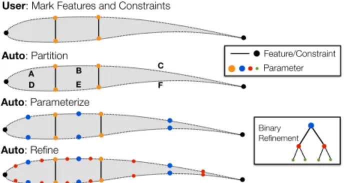
Figure 2:Progressive parameterization of an airfoil with discrete, hierarchical shape control refinement

In a progressive approach, a sequence of search spaces is generated, with a progressively increasing number of design variables, as illustrated in Figure 2. After optimizing within an initial low-dimensional search space, the shape control is refined, opening up new avenues for improvement, and the optimiza-tion continues in the higher-dimensional space. The basic idea is to first optimize in low-dimensional search spaces, allowing rapid design improvementa_, and then to introduce more dimensions to drive to-wards the optimal shape.b

To set up the problem, the designer specifies the objective function and constraints as usual. But instead of generating a static set of design variables, important designfeatures are marked, e.g. leading

edge, trailing edge, spar locations. Using these features as dividers, the surface is partitioned into regions, which are automatically parameterized. When parameterizing a curve such as an airfoil, initially a single design variable is placed at the midpoint of each region. Finer control is then gradually introduced as necessary. We adopt ahierarchical search space refinement technique, which implies a discrete approach to adding design variables, akin toh-refinement in mesh adaptation. This allows the shape control to be encoded as a binary tree, as depicted in Figure 2. This defines a clear sequence of search spaces that maintains strong regularity in the spacing of parameters.

! 2 Optimize Shape Refine Parameters Get candidates Shape derivatives Project gradients Geometry Modeler Rank ad a p ti v e XDDM Optimize Shape

Refine Search Space

Geometry Modeler

Optimize Shape

Refine Search Space

Geometry Modeler Determine Candidates

Rank Candidates

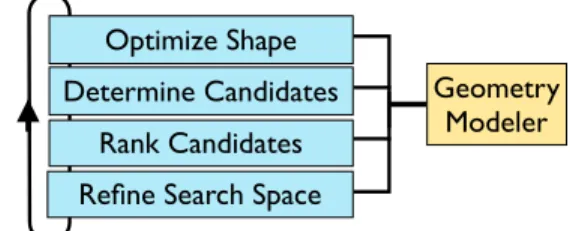
Figure 3: Optimization loop with concurrent search space refinement. The standalone geometry modeler is invoked via the XDDM protocol.3

As shown in Figure 3, the optimization process is now decomposed into a series of subproblems with fixed shape control, each of which is solved by a standard aerodynamic design framework. Once the current search space is sufficiently exploited, a search space refinement request is sent to the geometry modeler. Conceptually, both the static shape optimization framework and the geometry modeler can be viewed as standalone servers, although in practice there is a fair amount of interplay among them.

To address questions ofwhen andwhereto refine the shape control, a refinement strategy must be developed. In a companion research paper, we provide a more in-depth treatment of these components.1 _{In the next} sections we briefly cover the essential features of our shape control system.

a_{BFGS methods theoretically converge inO(N}

DV) search directions, meaning that having fewer degrees of freedom generally

leads to (initially) faster design improvement.

A. Triggering Search Space Refinement

To determine when to transition to a finer search space, we use a “trigger”, or stopping criterion, that terminates the optimization in the current search space and initiates a parameter refinement. A timely and robust trigger is critical for efficiency. Over-optimization on early parameterizations leads to sluggish design improvement and is a poor investment of resources, an observation also made by other authors.2, 18

One obvious and robust trigger is based on satisfying a tolerance on reduction of a norm of the objective gradients,c _{which indicates that optimality is being approached in the current search space. However, the} cutoff value is problem-dependent (especially with poorly scaled search spaces) making it difficult to set. For relatively smooth problems, we adopt a more aggressive approach. We monitor the rate of design improvement, as measured by the slope of the objective history with respect to search directions (see, e.g. Figure 8), and trigger a parameter refinement when this slope tapers to below a certain fraction of the maximum slope achieved under the current parameterization.d _{From an engineering perspective, this} makes sense: improvement in the objective function vs. cost is typically the figure of merit. However, for more difficult optimization problems, we observe that less aggressive triggers can be more effective, as the slope-based trigger can too hastily invoke a transition.

B. Uniform vs. Adaptive Refinement

The simplest and most robust approach to generate a sequence of parameterizations is to uniformly refine the search space, e.g. by binary subdivision of each tree, as shown in Figure 2. However, the distribution of parameters is then likely to be suboptimal, which can hurt efficiency. Alternatively,adaptive refinement aims to select themost effective parameterization, maximizing design improvement for a fixed number of design variables. This often reduces the total number of design variables required to find the optimum.

! 2 Optimize Shape Refine Parameters Get candidates Shape derivatives Project gradients Geometry Modeler Rank ad a p ti v e XDDM Optimize Shape

Refine Search Space

Geometry Modeler

Optimize Shape

Refine Search Space

Geometry Modeler Determine Candidates

Rank Candidates

Figure 4: Optimization loop with adaptive search space refinement. The API to the ge-ometry modeler is critical, as communication with it is required at every phase.

The adaptive optimization loop is depicted in Figure 4. To predict the relative effectiveness of the myriad possible shape control refinements, we extract gradient information the final adjoint solution(s) in the previous search space. Specifically, we compare norms of the local linearization of the objective and constraints tocandidate design variables, which provide some of the best information readily available on the parameters’ relative effectiveness. Naturally, this prediction is only local, because of the nonlinear design space. Furthermore, it is only as accurate as the PDE solutions. Nevertheless, our experiments show that larger gradients are strongly correlated with short term design improvements.

Choosing the best ensemble of N out ofNcand candidate parameters is a difficult combinatorial problem. We use a greedy

strategy, adding one parameter at a time from a priority queue ranked by the gradient norms. Much greater detail is given in the companion paper,1where we found this strategy to perform substantially better than random sampling and other simple methods.

The final consideration for adaptive refinement is the rate of parameter growth, which also has a critical impact on efficiency. Excessively high growth rates introduce large numbers of design variables, leading to a search space that is slow to navigate. However, slow parameter growth rates effectively “starve” the optimizer of degrees of freedom, stunting design improvement. We observe that the appropriate growth rate is problem-dependent. Simple problems, such as benchmark Case I, favor rapid growth rates, while more complex problems favor slower growth rates.

III.

Discretization Error Control Strategy

Controlling discretization error is an essential component of our system, because it enables a trade between cost and accuracy that dramatically accelerates the early phases of optimization. Our approach here is somewhat atypical. As shown in Figure 5, each design iteration is automatically meshed using output-based

c_{Or on satisfaction of the KKT conditions when constraints are present}

d_{This normalization by the maximum slope handles the widely differing scales that can be present in different objective}

Design 5 Final 103 104 Cells 0.05 0.1 Functional (J H ) 103 Cells 10-5 10-4 10-3 10-2 Error Error-Indicator | 2 | J ∆J 0 500 1000 1500 2000 MG Cycles 0 0.05 0.1 0.15 0.2 Functional /nobackupp8/ganders1/benchmarks/naca0012/prog3/param00/design000/M0.85A0B0_DP1 Iterative Convergence Thu Nov 20 14:42:07 2014 104 Cells 0.047 0.048 0.049 0.05 0.051 0.052 Functional (J H ) 103 Cells 10-5 10-4 10-3 10-2 Error Error-Indicator | 2 | J ∆J 0 500 1000 1500 2000 MG Cycles 0 0.05 0.1 0.15 0.2 Functional /nobackupp8/ganders1/benchmarks/naca0012/prog3/param00/design000/M0.85A0B0_DP1 Iterative Convergence Thu Nov 20 14:43:47 2014 10 3 10 4 Cells 0.05 0.1 Functional (J_H) 10 3 Cells 10 -5 10 -4 10 -3 10 -2 Error Error-Indicator | 2 | J ∆ J 0 500 1000 1500 2000 MG Cycles 0 0.05 0.1 0.15 0.2 Functional /nobackupp8/ganders1/benchmarks/naca0012/prog3/param00/design000/M0.85A0B0_DP1 Iterative Convergence Thu Nov 20 14:42:07 2014 103 104 Cells 0.05 0.1 Functional (J H ) 103 Cells 10-5 10-4 10-3 10-2 Error Error-Indicator | 2 | J ∆J 0 500 1000 1500 2000 MG Cycles 0 0.05 0.1 0.15 0.2 Functional /nobackupp8/ganders1/benchmarks/naca0012/prog3/param00/design000/M0.85A0B0_DP1 Iterative Convergence Thu Nov 20 14:42:07 2014 NACA0012 ±E Design 5 Design 59 103 104 Cells 0.05 0.1 Functional (J H ) 103 Cells 10-5 10-4 10-3 10-2 Error Error-Indicator | 2 | J ∆J 0 500 1000 1500 2000 MG Cycles 0 0.05 0.1 0.15 0.2 Functional /nobackupp8/ganders1/benchmarks/naca0012/prog3/param00/design000/M0.85A0B0_DP1 Iterative Convergence Thu Nov 20 14:42:07 2014 104 Cells 0.047 0.048 0.049 0.05 0.051 0.052 Functional (J H ) 103 Cells 10-5 10-4 10-3 10-2 Error Error-Indicator | 2 | J ∆J 0 500 1000 1500 2000 MG Cycles 0 0.05 0.1 0.15 0.2 Functional /nobackupp8/ganders1/benchmarks/naca0012/prog3/param00/design000/M0.85A0B0_DP1 Iterative Convergence Thu Nov 20 14:43:47 2014 10 3 10 4 Cells 0.05 0.1 Functional (J_H) 10 3 Cells 10 -5 10 -4 10 -3 10 -2 Error Error-Indicator | 2 | J ∆ J 0 500 1000 1500 2000 MG Cycles 0 0.05 0.1 0.15 0.2 Functional /nobackupp8/ganders1/benchmarks/naca0012/prog3/param00/design000/M0.85A0B0_DP1 Iterative Convergence Thu Nov 20 14:42:07 2014 103 104 Cells 0.05 0.1 Functional (J H ) 103 Cells 10-5 10-4 10-3 10-2 Error Error-Indicator | 2 | J ∆J 0 500 1000 1500 2000 MG Cycles 0 0.05 0.1 0.15 0.2 Functional /nobackupp8/ganders1/benchmarks/naca0012/prog3/param00/design000/M0.85A0B0_DP1 Iterative Convergence Thu Nov 20 14:42:07 2014 NACA0012

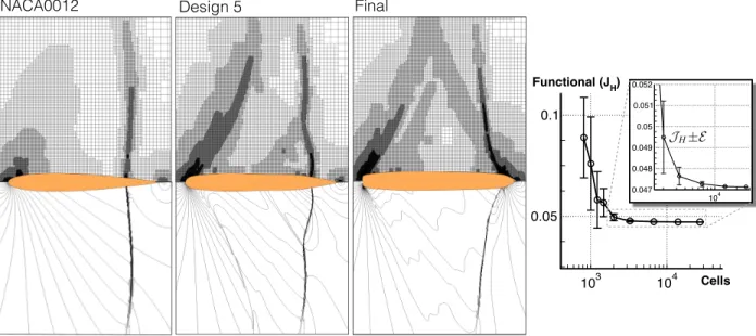
Figure 5: Top: Flow meshes adapted to accurately compute pressure drag at various airfoil shapes encountered

during optimization of Case I.Bottom: Mach contours.Right: Convergence of drag functional with mesh refinement for the baseline design. Bars indicate uncertainty in drag and properly bound the actual changes in the functional value.

e=|Jh(Qh) JH(QH)| (1)

Once the mesh refinement process is in the asymptotic region, the estimate of the remaining error can be expressed as E= 1 X i=0 1 4i= 4 3e (2)

assuming second order convergence, orE= 2efor first order convergence.

In contrast, under a typical fixed-mesh approach, an initial mesh convergence study is performed to determine a mesh appropriate for the baseline design, and then that same mesh is used for all designs. As the shape deviates more and more from the baseline, the initial mesh becomes less appropriate, leading to higher solution error as the design evolves. A convergence study on the final design does not solve the problem, because the optimization was being driven by flow solutions with ever-worsening accuracy, casting doubt on

the optimality of the final design. In our approach, accuracy is selectivelyincreasedwhile approaching the

optimum. This both saves expense up-front and also gives more credibility to the final design.

Talk about approach to adaptation for multiple functionals. Talk about error-tightening approach in more concrete terms. An advantage of non-tiered error control is the ability to stop anywhere and trust that result. C. Curve Parameterization by Direct Manipulation

D. Wing Parameterization

!

7 Baseline

Random Twist Stations Initial generators Target generators 22 24 26 28 30 2.4 2.6 2.8 3 3.2 3.4 3.6 Axis Fixed Twist Control stations

Figure 6: Wing planform parameterization

(Blender plugin)

For the two wing design problems, we use a deformer that interpolates both twist and airfoil section deformation in the spanwise direction. The deformer is illustrated in Figure 6. At each station a curve deformer (described in the previous sec-tion) sets the airfoil shape, after which the twist is applied. The twist is in the streamwise plane about a user-defined axis and is linearly interpolated between successive stations. Control sta-tions can be arbitrarily spaced along the span, but for this work we maintain strict regularity by refining only at the midpoints between consecutive stations.

5 of 13

American Institute of Aeronautics and Astronautics Figure 5: Top: Flow meshes adapted to accurately compute pressure drag at various airfoils encountered during optimization for Case I. Bottom: Mach contours. Right: Convergence of drag functional with mesh refinement for the baseline design. Bars indicate uncertainty in drag and asymptotically bound the actual changes in the functional value.

adaptive refinement that seeks to reduce error in the objective and constraint functionals.2_{Thus we obtain} mesh convergence information foreach design. Naturally,an indiscriminate application of tight error control would greatly increase the computational expense. However, by tracking the output error and comparing it to the evolution of the objective function, we can selectively reduce solution the accuracy during the early stages of optimization, when large design improvements are possible even with coarse simulations. The resolution can then be automatically sharpened as the design approaches optimality. From an engineering perspective, this approach has the added benefit of providing an estimate of the error on the functionals of interest throughout design.

To estimate the discretization error in an aerodynamic functional (e.g. lift or drag), we use an adjoint-weighted residual approach.19_{An example of convergence of this error estimate with mesh refinement is shown} in the right frame of Figure 5. For most practical studies involving multiple design functionals, we construct acombined mesh adaptation functional that seeks to adequately resolve all the outputs. For example, in Case III (twist optimization) we adapt the mesh to resolve the span efficiency factor, which leads to a mesh that is well-balanced to compute both lift and drag.

One tremendous advantage of output-based meshing at each design iteration is that it removes the burden of having to hand-craft flow meshes for optimization. In contrast, in the typical approach, one tries to construct a fixed mesh that anticipates how critical flow features will move as the design progresses. As the shape deviates more and more from the baseline, the fixed mesh becomes less appropriate, often leading to higher solution error as the design evolves. In our approach, accuracy is selectively increased while approaching the optimum. This reduces up-front costs (in both user and computational time) and also gives more credibility to the optimality of the final design.

IV.

Inviscid Benchmarks

The two inviscid problems (Cases I and III) are presented first. Case I involves drag minimization for a symmetric non-lifting airfoil that must contain the baseline shape. Case III is a twist optimization problem for induced drag minimization subject to a lift constraint. Throughout each optimization we monitor objective convergence with shape control refinement, constraint satisfaction, and error in the outputs. A few ancillary details, such as optimizer settings, are given in the Appendix.

A. Case I. Symmetric Transonic Airfoil Design

The first test case is a geometrically-constrained drag minimization problem (_J =CD). The starting airfoil is a modified NACA 0012 (henceforth “N0012m”), where the trailing edge is made sharp.e _{The design Mach} number is 0.85, while the angle of attack is fixed atα= 0◦_{. Additionally, the final airfoil shape mustcontain} the original airfoil. This constraint is satisfied when y _≥yN0012m everywhere on the upper surface, and inversely on the lower surface. Because the solution must be symmetric, we work only in the upper half of the domain with a symmetry boundary condition at y = 0. The farfield boundaries are placed 96 chords away in each coordinate direction.

1. Shape Parameterization 0 0.2 0.4 0.6 0.8 1 -0.08 -0.06 -0.04 -0.02 0 0.02 0.04 0.06 0.08 Initial Final Control Points Level 1 Level 2 Level 0

Figure 6:Case I: Initial parameterization with 7 design variables, generated by twice uniformly refining a 1-DV parameterization (lower half generated by symmetry)

To deform the airfoil we use a “direct manipulation” approach, where we explicitly specify the deformation of certain “pilot points” along the airfoil, as shown in Figure 6. These points serve as the design variables, while deformation of the remain-der of the curve is smoothly interpolated using radial basis functions.f

For this problem, initially a single pilot point is placed on the top surface, as shown in Figure 6 (black dot). Practically

speaking, we observe that it is more efficient to start with several design variables, rather than a truly minimal set, so we immediately perform two uniform refinements before beginning optimization. The shape control is clustered towards the leading edge by transforming the arc-length parametric spaceg_{. During shape control} refinement, new pilot points are placed at the midpoints between existing ones. The midpoint is measured in the transformed space, so in physical space, they are also biased towards the leading edge.

−0.08 −0.04 0.00 0.04 0.08 Scaled T o scale 0.00 0.25 0.50 0.75 1.00 x/c −1.6 −0.8 0.0 0.8 Cp NACA0012 Optimized

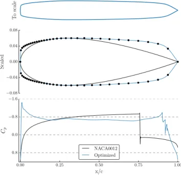
Figure 7: Case I: Final airfoil shape and pressure profile. Black dots indicate the location of the final 31 shape control parameters.

To handle the containment constraint, we set the lower bound of each shape pa-rameter to the corresponding local thick-ness of the N0012m. The direct manipu-lation approach guarantees that the airfoil will exactly interpolate these pilot points. Regions between the shape control parame-ters may temporarily violate the contain-ment constraint, but these violations get squeezed out as more parameters are added. In keeping with our adaptive approach, the containment constraint becomes more pre-cise as the search space is refined.

2. Optimization Results

Figure 7 shows the final optimized airfoil and its pressure profile. Two features are most noticeable. First, the leading edge has become extremely blunt. In fact, after every successive parameter refinement, the nose became blunter, limited only by the first shape parameter’s proximity to the leading edge. This is the expected optimal result for

this problem, though naturally this shape would have poor off-design performance and poor viscous perfor-mance. By the final design, the containment constraint is satisfied everywhere (not just at the interpolation points).

e_{Via modification of thex}4_{coefficient: y=±0.6 0.2969}√_{x−0.1260x−0.3516x}2_{+ 0.2843x}3_−0.1036x4

f_{We choose the basis functionφ=r}3_{here, primarily because it requires no local tuning parameters, making it more amenable}

to automation.20–23

D ra g (c ou n ts ) 0 6 12 18 24 30 36 42 48 54 60 Search direction 0 100 200 300 400 500 O b jecti ve P0: 7DV P1: 15DV P2: 31DV 0 6 12 18 24 30 36 42 48 54 60

Search direction

0 100 200 300 400 500

O

b

jecti

ve

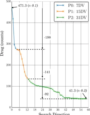
P0: 7DV P1: 15DV P2: 31DV Search Direction 471.3 (± 0.1) -198 41.3 (± 0.3) -141 -92

Figure 8:Case I: Objective convergence

Figure 8 shows the convergence of the objective function over 60 search directions, and over 3 parameterization levels. The parameterization was automatically refined (i.e. with no user intervention) when the objective slope tapered to 20% of its maximum slope. The final level contained 31 de-sign variables. The drag was reduced from the baseline 471 counts to 41.3 counts. An additional refinement to 63-DVs proved unable to further improve the design. The final de-sign is probably close to optimal, as demonstrated by the diminishing return on each additional parameter refinement visible in Figure 8. Some further improvement is likely pos-sible, but even the small amount of remaining discretization error combined with the very high-dimensional design space makes further improvement extremely difficult.

Figure 9 compares the initial and final meshes, which were automatically adapted to reduce error in drag. Interme-diate designs generated radically different mesh refinement patterns (see Figure 5 for the final design of the 7-DV param-eterization level). The refinement patterns reflect movement of the shock and changes in the width of the supersonic re-gion. For the final design, the adjoint-based mesh adaptation process provided an estimate of the remaining error in drag of about 0.3 counts (<3_·10−5 _inC

D). The output-based mesh adaptation performed a mesh refinement study at each

design iteration, yielding convergence similar to that shown in the right frame of Figure 5. This level of error was roughly constant throughout the optimization (see Table 1), giving high credibility to the final design. The cell count required to meet the error tolerance gradually increased throughout optimization. This indicates that the optimization drove the design to become more sensitive to the mesh discretization, as the shock weakened and numerical dissipation became more noticeable.

Baseline Final

Mach

0.85 1 1.15

Figure 9: Case I: Comparison of baseline and final meshes. The mesh refines the regions most important for computing drag, primarily focusing on the leading edge expansion and shock. Meshing requirements to achieve the same error tolerance generally increased with optimization: the baseline mesh has 26K cells (upper half only), while the final design has 61K cells.

Table 1:Case I drag reduction with optimization. All drag measured in counts (CD·104) Baseline 7 DV 15 DV 31 DV CD 471.3 273.8 133.0 41.3 Error estimate _±0.1 _±0.1 _±0.1 _±0.35 Cells 26 K 49 K 50 K 61 K 3. Sensitivity to Farfield

The optimization process radically increased the sensitivity of the flow to the farfield boundary distance. The initial N0012m, with its relatively confined regions of supersonic flow, is quite lenient with respect to the farfield boundary location.h _{An initial domain size study indicated that a farfield distance of 24 chords} was sufficient to resolve drag to within 2 counts of the value obtained using 96-chord distances. However, the final design’s carefully tuned shock structure (see Figure 7) could not be reliably resolved with farfields nearer than about 96 chords. We observed that near the final design, an inadequate farfield distance or mesh resolution can lead to an alternate solution with stronger shocks that roughly double the amount of drag! In our approach, we adapt the mesh to suit each design iteration, but always within a fixed domain size. To combat this changing sensitivity, a more comprehensive approach might periodically re-evaluate the sensitivity to farfield boundary distance, expanding the domain as necessary.

B. Assessment of the Approach

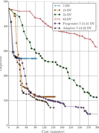
0 30 60 90 120 150 180 210 240 270 300 Cost (minutes) 0 100 200 300 400 500 O b jecti ve 7-DV 15-DV 31-DV 63-DV Progressive 7-15-31 DV Adaptive 7-12-22 DV

Figure 10:Case I: Effectiveness of different parameteriza-tion schemes, showing design improvement vs. wall-clock time. ×-marks indicate search space refinements on the progressive and adaptive methods. (All cases used identical error control settings.)

A progressive, automated approach has clear ad-vantages in terms of user time and thoroughness. However, a naive implementation can also be very costly.Before proceeding to the remaining bench-marks, it is worth pausing to evaluate the computa-tional performance of our approach. To solve Case I, we used a constant error target throughout the opti-mization to satisfy the benchmark discussion group requirements of having an accurate flow solutions throughout design. Now, however, we show that the bulk of the design improvement can be obtained using quite coarse meshes, with substantial error con-trol only being applied near the end to resolve the design landscape near the optimum.

1. Adaptive vs. Fixed Search Spaces

We observe that progressive parameterization strongly outperforms any of the fixed search spaces on Case I. To give a rough sense of performance, Fig-ure 10 plots design improvement versus wall-clock time for solving Case I with various parameteriza-tions on four cores of a laptopi_{. The uniform} refine-ment scheme (labeled “progressive”) and the adap-tive approach (which resulted in fewer design vari-ables) both achieved faster and deeper overall design improvement than any coarse or fine fixed param-eterization. As expected, low-dimensional search spaces support limited design improvement, while high-dimensional spaces take much longer to navi-gate. On the finest (63-DV) fixed parameterization,

h_{The farfield boundary state is enforced weakly via 1-D Riemann invariants without using circulation correction.}

0 40 80 120 160 200 240 280 320 Cost (minutes) 0 100 200 300 400 500 600 Ob jectiv e

Constant Error Tol. Progressive Error Control

(a)Design improvement vs. wall-clock time. Only meshing, flow solver, and adjoint solutions timed: geometry genera-tion excluded. Shaded bands on the progressive case indi-cate discretization uncertainty in the functional. ×-marks denote search space refinements.

106 105 104 Functional Error Tolerance 0.0 50.0 k 100.0 k # Cells 0 10 20 30 40 50 60 70 80 90 Design Iteration 0 5 10 15 20

Mesh Refinement Depth

106 105 104 103 102 Functional Error Tolerance 0.0 10.0 k 20.0 k 30.0 k # Cells 0 20 40 60 80 100 120 140 Design Iteration 0 5 10 15 20

Mesh Refinement Depth

Design Iteration Design Iteration

(b) Constant error tolerance and actual error estimate history 106 105 104 Functional Error Tolerance 0.0 50.0 k 100.0 k # Cells 0 10 20 30 40 50 60 70 80 90 Design Iteration 0 5 10 15 20

Mesh Refinement Depth

106 105 104 103 102 Functional Error Tolerance 0.0 10.0 k 20.0 k 30.0 k # Cells 0 20 40 60 80 100 120 140 Design Iteration 0 5 10 15 20

Mesh Refinement Depth

Design Iteration Design Iteration

(c) Progressive error control and actual error estimate history 10 6 10 5 10 4 10 3 10 2 Functional Error Tolerance Functional Error Tolerance 0.0 50.0 k 100.0 k # Cells # Cells 0 20 40 60 80 100 120 140 160 Design Iteration 0 5 10 15 20

Mesh Refinement Depth Mesh Refinement Depth

#

C

el

ls

Design Iteration Constant tolerance Progressive control

(d) Cell count history

Figure 11:Case I: Comparison of fixed error control vs. progressive error control. Both cases were performed with identical parameterization strategies and on identical hardware (2013 MacBook Pro with a 2.6GHz Intel Core i7 and 16GB of memory).

which stalled quite early, the optimizer may simply be unable to navigate the design space, as also reported by Carrieret al.on this problem.12_{Starting in a coarse design space appears to smooth the navigation early} on, leading to a more robust search process, an observation we also expand upon in the companion paper.1 On this problem, the adaptive approach (which results in fewer design variables) is slightly faster than the progressive approach for most of the process. This speedup is largely due to the smaller number of shape derivative calls to the geometry modeler and gradient projections, and perhaps partly due to the lower dimensional design space. For slow geometry modelers, this advantage could be even more significant. However, factors such as the trigger, rate of variable introduction, indicator, scaling, and path-dependence make it difficult to draw firm conclusions about the computational advantage of adaptive refinement vs. uniform refinement from such a cursory study.

2. Error Control Strategy

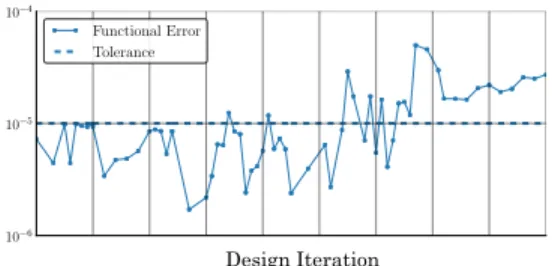
The adjoint-based mesh refinement technique used here provides a mesh refinement study and discretization error estimate along with every functional evaluation. While using tight error control throughout the opti-mization can lend credence to the process, blind application can result in unnecessary expense. Consulting Figure 11a, we see that a progressive error-targeting scheme has a significant cost advantage over the static error approach that we used for the Case I benchmark. Early in design, large improvements can be guided even with fairly coarse meshes. By adopting very loose tolerances early on (Figure ??), the early stages of

optimization are greatly accelerated, without sacrificing accuracy near the optimum.

Our automatic adaptive meshing approach is especially advantageous for problems like Case I, which exhibit substantial, unpredictable differences between the initial and final designs. However, near the optimum successive design iterations are often quite similar. Warm-starting the meshing and flow solutions for nearby designs is an obvious avenue for further acceleration.

C. Case III. Subsonic Wing Twist Optimization

We defer Case II momentarily to first consider the other inviscid problem, Case III. This is a wing twist optimization problem, where the airfoil section and planform remain unmodified. The objective is to reduce drag (J = CD), subject to a lift constraint (CL = 0.375). The flight condition is Mach 0.5. Since the flow is shock-free, this is strictly an induced drag reduction problem. Assuming the span efficiency factor cannot exceed 1.0, as non-planar deformations are minimal with the twist applied about the trailing edge, the minimum possible drag is about

CDmin = C2 L πe0ÆR =0.375 2 6.0π = 74.6 counts (1)

However, as the wing is untapered, and twist is about the trailing edge, we do not expect that the optimal design will recover a precisely elliptical lift distribution. Additionally, we observed a very small shock on the wing tip near the trailing edge, where the flow accelerates around the tip to the top surface, which may further reduce the possible drag gains.

The baseline design has only about 77 counts of drag. Unlike Case I, where the objective was reduced by a factor of ten, here the possible improvements are very small, which places high demands on the accuracy of the flow solution.24 _{We compute adjoint solutions for the drag and lift functionals to compute their gradients,} allowing the nonlinear lift constraint to be treated exactly by SNOPT.

1. Shape Parameterization

The baseline geometry is a straight, unswept, untwisted wing, generated by extruding the N0012m section three chord lengths and capping the tip by a simple revolution. For this problem we use a deformer that interpolates twist between arbitrary spanwise stations. The twist is in the streamwise plane about the trailing edge and is linearly interpolated between successive stations. Control stations can be arbitrarily spaced along the span, but for this problem we maintain strict regularity by refining only at the midpoints between consecutive stations. We allow the global angle of attack to vary and therefore hold the twist fixed at the wing root. The first parameterization (“P0”) has two twist stations, located at the tip and mid-span. To generate the second level (“P1”), new twist stations are added at the midpoints between existing ones.

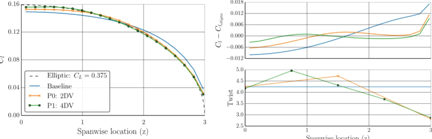
0.00 0.04 0.08 0.12 0.16 Cl Elliptic:CL= 0.375 Baseline P0: 2DV P1: 4DV 0.012 0.006 0.000 0.006 0.012 0.018 Cl Clel li p ti c 3.0 3.5 4.0 4.5 5.0 T w ist 0.00 0.04 0.08 0.12 0.16 Cl Elliptic:CL= 0.375 Baseline P0: 2DV P1: 4DV 0.012 0.006 0.000 0.006 0.012 0.018 Cl Clel li p ti c 0 1 2 3 Spanwise location (z) 2.5 3.0 3.5 4.0 4.5 5.0 T w ist 0.00 0.04 0.08 0.12 0.16 Cl Elliptic:CL= 0.375 Baseline P0: 2DV P1: 4DV 0.012 0.006 0.000 0.006 0.012 0.018 Cl Clel li p ti c 0 1 2 3 Spanwise location (z) 2.5 3.0 3.5 4.0 4.5 5.0 T w ist

Figure 12:Case III: Twist optimization results. Left: Sectional lift distribution profiles. Top right: Deviation from elliptic distribution. Bottom right: Twist distribution

10 of 18

2. Mesh and Error Control

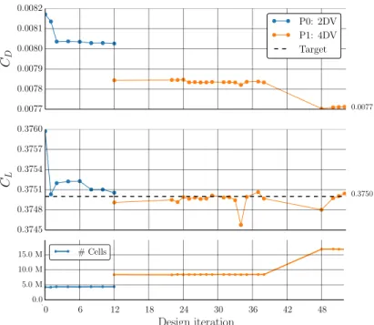
The error control scheduling was set to coincide with the parameterization refinements, and the farfield boundaries were placed at 48 chords away. In the first design space, the resulting adapted meshes contained about 5 million cells, but for the second design space, the meshes contained 10-15 million cells to meet the tighter error tolerance.

3. Optimization Results 0.0077 0.0078 0.0079 0.0080 0.0081 0.0082 CD 0.0077 P0: 2DV P1: 4DV Target 0 6 12 18 24 30 36 42 48 Design iteration 0.3745 0.3748 0.3751 0.3754 0.3757 0.3760 CL 0.3750 103 102 Functional Error Tolerance 0.0 5.0 M 10.0 M 15.0 M # Cells 0 6 12 18 24 30 36 42 48 Design Iteration 0 5 10 15 20

Mesh Refinement Depth

0.0077 0.0078 0.0079 0.0080 0.0081 0.0082 CD 0.0077 P0: 2DV P1: 4DV Target 0 6 12 18 24 30 36 42 48 Design iteration 0.3745 0.3748 0.3751 0.3754 0.3757 0.3760 CL 0.3750

Figure 13:Case III: Top: Convergence of drag. Middle: Convergence of lift. Bottom: Cell count history

Figure 12 shows the main results of the op-timization. The lift distribution rapidly approaches an elliptical shape, with only very small discrepancies at the tip, due to the untapered section, and at the root, which compensates to exactly match lift. Figure 13 shows the convergence of the lift and drag functionals. Because a coarser mesh was used in the initial de-sign space, there is a jump in functional values when transitioning to the finer de-sign space. By the end lift is satisfied and drag is reduced. To accurately de-termine the total improvement, we per-formed an additional high resolution anal-ysis on the initial and final designs. Fig-ure 14 shows the convergence of span effi-ciency factor with mesh refinement for the initial and final designs. In terms of drag, the initial design hadCD = 77.2 counts at CL = 0.3762, or in terms of span ef-ficiency e= 0.972_±0.003. By the final design this was improved toCD= 76.1 at

CL= 0.3762 (e= 0.987±0.003).

10

6

10

7

Cells

0.5

0.6

0.7

0.8

0.9

1

Span Efficiency Factor

10

6

10

7

Cells

10

-3

10

-2

10

-1

Error

Error-Indicator |η| 2 | J_C - J_H | ∆J

0

500

1000

1500

2000

0

0.2

0.4

0.6

0.8

1

Functional

maxRef = 16

Iterative Convergence

Tue Nov 25 14:07:40 2014

10

6

10

7

Cells

0.5

0.6

0.7

0.8

0.9

1

Span Efficiency Factor

10

6

10

7

Cells

10

-3

10

-2

10

-1

Error

Error-Indicator |η| 2 | J_C - J_H | ∆J

0

500

1000

1500

2000

0

0.2

0.4

0.6

0.8

1

Functional

maxRef = 16

Iterative Convergence

Tue Nov 25 13:57:51 2014 107 Cells 0.9 0.92 0.94 0.96 0.98 1

Span Efficiency Factor

106 107 Cells 10-3 10-2 10-1 Error Error-Indicator |η| 2 | JC - JH | ∆J 0 500 1000 1500 2000 MG Cycles 0 0.2 0.4 0.6 0.8 1 Functional /nobackupp8/ganders1/benchmarks/twist/marian_setup_6/param01/BEST/M0.5A4.50345B0_DP1 maxRef = 16 Iterative Convergence Tue Nov 25 13:56:59 2014 107 Cells 0.95 0.96 0.97 0.98

Span Efficiency Factor

106 107 Cells 10-3 10-2 10-1 Error Error-Indicator |η| 2 | J_C - J_H | ∆J 0 500 1000 1500 2000 MG Cycles 0 0.2 0.4 0.6 0.8 1 Functional maxRef = 16 Iterative Convergence Tue Nov 25 13:54:56 2014

(a)Baseline design

10

6

10

7

Cells

0.5

0.6

0.7

0.8

0.9

1

Span Efficiency Factor

10

6

10

7

Cells

10

-3

10

-2

10

-1

Error

Error-Indicator |η| 2 | J_C - J_H | ∆J

0

0.2

0.4

0.6

0.8

1

Functional

maxRef = 16

Iterative Convergence

Tue Nov 25 14:07:40 2014 107 Cells 0.95 0.96 0.97 0.98

Span Efficiency Factor

106 107 Cells 10-3 10-2 10-1 Error Error-Indicator |η| 2 | J_C - J_H | ∆J 0 500 1000 1500 2000 MG Cycles 0 0.2 0.4 0.6 0.8 1 Functional maxRef = 16 Iterative Convergence Tue Nov 25 13:54:56 2014

10

6

10

7

Cells

0.4

0.5

0.6

0.7

0.8

0.9

1

Span Efficiency Factor

10

6

10

7

Cells

10

-2

10

-1

Error

Error-Indicator |η| 2 | J_C - J_H | ∆J

0

500

1000

1500

2000

0

0.5

1

1.5

2

Functional

maxRef = 16

Iterative Convergence

Wed Nov 26 16:42:14 2014 106 107 Cells 0.9 0.92 0.94 0.96 0.98 1

Span Efficiency Factor

106 107 Cells 10-2 10-1 Error Error-Indicator |η| 2 | J_C - J_H | ∆J 0 500 1000 1500 2000 MG Cycles 0 0.5 1 1.5 2 Functional /nobackupp8/ganders1/benchmarks/twist/final_analysis maxRef = 16 Iterative Convergence Wed Nov 26 16:43:09 2014 (b) Final design

Figure 14:Case III: Convergence of span efficiency factor with mesh refinement

11 of 18

Table 2:Case III results.

Distance from Root 0c 0.6c 1.2c 1.8c 2.4c 2.7c 2.85c 2.97c 3.0c

Twist (o_{) 4.2 4.8 4.5 4.1 3.5 3.2 3.0 2.9 2.9}

Sectional Lift (2cl/b) 0.156 0.156 0.146 0.126 0.094 0.069 0.050 0.030 0.0

V.

Viscous Benchmarks

We now turn to the two RANS optimization benchmarks. As our design framework uses an inviscid solver, the results will not be directly comparable to other viscous results. For Case II, we modify the design problem slightly to achieve better viscous performance with an inviscid optimization approach. The modification was guided by viscous analysis from a recently developed 2D Cartesian RANS approach by Berger and Aftosmis.25 A. Case II. Transonic Airfoil Design

0.05 0.00 0.05 S ca led T o sca le 0.00 0.25 0.50 0.75 1.00 x/c 1.8 1.2 0.6 0.0 0.6 Cp RAE 2822 3 1 4 5 2 6 Binary Refinement

Figure 15: Case II: Initial 6-DV parameteri-zation and uniform refinement.

Case II revisits transonic airfoil design (Mach 0.734), but this time with more realistic design constraints. The objective is again to reduce the drag (J = CD), while constraints are imposed on lift, pitching moment (which is initially violated) and the areaA:

CL = 0.824

CM ≥ −0.092

A_≥ARAE≈0.07787c2

We compute adjoint solutions for the drag, lift and pitching moment functionals to compute their gradients. The area is computed on the discrete surface, and the constraint gradients are differentiated analytically.

The baseline shape is the RAE 2822 airfoil. We parameterize the deformation with the same curve deformer as in Case I. In addition to angle of attack, there are initially six shape parameters, as shown in Figure 15. Shape control refinement is uniform. For discretization error control, we set a lower tolerance in the first search space, and then tighten it to target±0.5 counts of drag on the second level.

1. Inviscid Optimization: Trial 1 (Pure Inviscid Design)

Figure 16 shows the results of driving the optimization with inviscid flow solutions at the specified flight conditions. SNOPT rapidly drove down the drag, but after several search directions without noticeably improving the aerodynamic constraints, it increased its internal constraint weights, rapidly driving the pitching moment and lift to be satisfied. The shock is nearly eliminated even under the first parameterization. After refining to 14-DVs (and simultaneously tightening the discretization error tolerance), the shock is completely eliminated. An additional refinement to 30-DV’s did not yield any further improvent for reducing the negligible remaining inviscid drag.

2. Viscous Analysis

To check the viscous performance of this design, we computed the flow using the Cartesian RANS solver mentioned above,25_{with a Spalart-Allmaras turbulence model at Re}

c= 6.5 million. The RANS solution is shown in Figure 17. The inviscidly-designed airfoil does have superior viscous performance to the original RAE. Consulting Table 3, the viscousCD is reduced by 90 counts. However, the presence of the boundary layer increased the angle of attack necessary to achieveCL= 0.824, resulting in higher Mach numbers over the top surface and thus the presence of a moderately strong shock.

−0.06 −0.03 0.00 0.03 0.06 0.09 Scaled T o scale 0.00 0.25 0.50 0.75 1.00 x/c −1.8 −1.2 −0.6 0.0 0.6 Cp RAE 2822 P0: 6 DV P1: 14 DV

(a) Top: Final airfoil to scale. Middle: Final parame-terization. Bottom: Pressure profile at the end of each optimization level. 0.000 0.002 0.004 0.006 0.008 0.010 CD 0.0007 P0: 6 DV P1: 14 DV Min Target 0.76 0.78 0.80 0.82 0.84 0.86 CL 0.8240 −0.12 −0.08 −0.04 CM -0.0920 0 20 40 60 80 100 Design iteration 0.0775 0.0800 0.0825 0.0850 0.0875 0.0900 Area 0.0779

(b) Convergence of aerodynamic functionals (plotted at successful search directions). The first level used some-what coarser flow meshes, visible in the subtle disconti-nuity in drag where the parameterization is refined.

Figure 16:Case II: Trial 1 (inviscid) results across two parameterization levels

Figure 17:Case II: Reynolds-averaged Navier-Stokes anal-ysis of the inviscid design, showing pressure contours and colored by Mach number. (CL= 0.824,M0.734,Re= 6.5

million)

At these flight conditions under the assumption of inviscid flow, a wide range of shapes eliminate the shock while satisfying the constraints. However, most of these designs have poor viscous performance. To encourage the optimizer to prefer shapes with bet-ter viscous performance, we follow the approach used by Smithet al.26_{and earlier by Campbell.}27_Briefly, we mimic the shallower effectivetrailing edge slope present in the RANS analysis, by applying a small upward cubic deflection to the last 20% of the airfoil at every design iteration during inviscid design:

y=y+ x−0.8 0.2 3 sin(θ) (2)

where we usedθ= 0.3◦. This forces the optimizer and inviscid solver to compensate for a shallower effective trailing edge camber line. Naturally, the fictitious deflection is then removed when analyzing the final design under viscous conditions. To help exclude irrelevant designs with little inviscid penalty but poor viscous performance, for this trial we also added three thickness preservation constraints by removing three design variables in the initial search space.

−0.08 −0.04 0.00 0.04 0.08 Scaled T o scale 0.00 0.25 0.50 0.75 1.00 x/c −1.8 −1.2 −0.6 0.0 0.6 Cp Baseline P0: 3DV P1: 11DV

(a)Top: Final airfoil to scale. Middle: Final parameter-ization. (Note the deflection at the trailing edge, which is appliedafter the curve deformation.)Bottom: Inviscid pressure profile 0 0.2 0.4 0.6 0.8 1

x/C

-2 -1 0 1 2

Cp

Viscous

Inviscid

C

L

= 0

.

824

, M

0

.

734

Inviscid

Viscous

(b) Pressure profile for final design

(c)Viscous solution of final design, showing isobars, with color indicating Mach number (CL = 0.824, M0.734,

Re= 6.5 million) 0 0.1 0.2 0.3 0.4 0.5 0.6 0.7 0.8 0.9 1 1.1 x/C 0 0.001 0.002 0.003 0.004 0.005 0.006 0.007 0.008 0.009 0.01 Cf (d)Friction coefficientCf.

Table 3:Case II drag reduction with optimization.

Solver Baseline Trial 1 Trial 2

Inviscid CD 0.0068 0.0007 0.0007 Error _±0.0001 _±0.00005 _±0.00006 Cells 21K 12K 27 K αtrim 1.73◦ 2.28◦ 2.72◦ Viscous CD 0.0252 0.0162 0.0124 αtrim 3.45◦ 3.60◦ 2.61◦

Figure 18 shows the results of this second optimization. Although the new inviscid design (top left frame) is not fully shock-free, the viscous performance (other frames) is substantially better, leading to about 124 counts of drag, or 38 counts lower than the purely inviscid design. As show in Table 3, the primary difference is that this design has a much better match between the trimmedαfor the inviscid analysis and for the viscous analysis, leading to similar behavior over

the front region, and importantly, similar shock placement.

B. Case IV. Transonic Wing Design

Case IV is a wing design optimization problem at Mach 0.85. The objective is to reduce drag (_J =CD), subject to a lift constraint and a pitching moment constraintj_{, which is initially violated. The baseline} geometry is the Common Research Model wing (henceforth “CRM”), scaled so that the mean aerodynamic chord has unit length. The planform is fixed, while variation in the vertical direction is permitted, including airfoil design and sectional twist. The twist is about the trailing edge and is fixed at the root, while the angle of attack is permitted to vary. The wing is required to maintain its initial volumeV0 and also to maintain at least 25% of its original local thicknesst0everywhere. To approximate this continuous thickness constraint, we used a 10_×10 grid of constraints distributed evenly across the planform.

Axis P0 P1 22 24 26 28 30 2.4 2.6 2.8 3 3.2 3.4 3.6 22 24 26 28 30 2.4 2.6 2.8 3 3.2 3.4 3.6 Twist

P0

P1

x

y

Figure 19:Case IV: First two shape control levels (8-DV and 26-DV)

The full optimization problem is

minCD

CL= 0.5

CM ≥ −0.17

V _≥V0≈0.26291

ti≥0.25ti0∀i

We solve this problem unmodified, but at invis-cid conditions to demonstrate our design approach. Thus results will not be directly comparable to vis-cous design results.

1. Shape Parameterization

For this problem, we use a deformer similar to that used in Case III, but here it interpolates both twist and airfoil section deformation independently. At each station a curve deformer (identical to the setup used for Cases I and II) deforms the airfoil shape, after which the twist is applied. Each airfoil param-eter has a bump-shaped deformation mode (based on RBF interpolation) that is mostly confined to the region between its neighboring points, while main-taining smoothness. As before, the twist is in the

streamwise plane about the trailing edge and is linearly interpolated. Control over airfoil sections and twist can happen at different stations, allowing for “anisotropic” shape control. For example, the twist control may have a higher spanwise resolution than the airfoil control. Similarly, each airfoil control station can offer different shape control resolution.

0.0100 0.0125 0.0150 0.0175 0.0200 0.0225 CD 0.0116 P0: 8DV P1: 26DV P2: 70DV Min Target 0.490 0.495 0.500 0.505 CL 0.4993 0 8 16 24 32 40 48 56 64 72 Design iteration −0.26 −0.24 −0.22 −0.20 −0.18 −0.16 CM -0.1694

Figure 20: Case IV: Convergence of aerodynamic func-tionals (only plotted at successful search directions).

Figure 19 shows the first two search spaces (“P0” and “P1”). The initial parameterization allows twist at the tip and break (fixed at the root) and very rough camber and thickness control (two control points each on the root, break and tip sections). There are initially eight shape design variables, plus the angle of attack. To refine the parameterization, we add new control stations at the spanwise mid-points between the existing stations, and simultane-ously add new airfoil control points at the midpoints between existing control points. Two additional pa-rameterization levels (“P1” and “P2”) are generated by uniform refinement, resulting in 26 and 70 geo-metric design variables, respectively.

2. Optimization Results

Figure 20 shows the convergence of the aerodynamic functionals over the three parameterization levels. Under “P0”, the initially violated pitching constraint is driven to satisfaction. To do this, large airfoil de-formations are enacted, as shown in Figure 21 (blue

−0.24 −0.16 −0.08 0.00 0.08 0.16 S ca le d T o sc al e 0.0 0.3 0.6 0.9 1.2 1.5 x/c −1.0 −0.5 0.0 0.5 Cp Baseline P0: 8DV P1: 26DV P2: 70DV (a) 2.35% −0.06 −0.03 0.00 0.03 0.06 0.09 S ca le d T o sc al e 0.75 1.00 1.25 1.50 1.75 x/c −1.0 −0.5 0.0 0.5 Cp Baseline P0: 8DV P1: 26DV P2: 70DV (b)26.7% 0.025 0.050 0.075 0.100 0.125 0.150 S ca le d T o sc al e 1.50 1.65 1.80 1.95 2.10 2.25 x/c −1.0 −0.5 0.0 0.5 Cp Baseline P0: 8DV P1: 26DV P2: 70DV (c)55.7% 0.075 0.100 0.125 0.150 0.175 0.200 S ca le d T o sc al e 1.95 2.10 2.25 2.40 2.55 x/c −1.0 −0.5 0.0 0.5 Cp Baseline P0: 8DV P1: 26DV P2: 70DV (d)69.5% 0.16 0.18 0.20 0.22 0.24 0.26 S ca le d T o sc al e 2.40 2.55 2.70 2.85 x/c −1.0 −0.5 0.0 0.5 Cp Baseline P0: 8DV P1: 26DV P2: 70DV (e)82.8% 0.24 0.26 0.28 0.30 0.32 S ca le d T o sc al e 2.7 2.8 2.9 3.0 3.1 x/c −1.0 −0.5 0.0 0.5 Cp Baseline P0: 8DV P1: 26DV P2: 70DV (f )94.4%

lines), with a resulting sharp increase in drag. After adding more shape control resolution, the drag is rapidly driven down nearly to the initial value, while nearly satisfying the constraints. The airfoil sections (Figure 21, orange lines) relax to more subtle changes from the baseline shape. The thickness and volume constraints are met at every design iteration. Overall, all of the constraints are nearly satisfied by the end, with only a slight drag penalty associated with having to meet the initially violated pitching moment constraint. We did not yet analyze the performance of the inviscidly optimized wing with a viscous flow solver. It is possible that a modification of the trailing edge (as in Case II) would improve the viscous performance.

VI.

Summary

We presented results for four optimization benchmark problems. On the two inviscid design problems, expected results were recovered. For Case I, our final shape is nearly identical to shapes seen by previous participants,11–15_{with similar or superior drag performance (reduction of 10}

×from the baseline). For Case III, although potential improvements were quite small, by optimizing the wing twist, we drove the lift distribution closer to elliptic. On Case II, we showed how an inviscid design approach with slight problem modifications was able to reduce the RANS-analyzed drag by a factor of two (128 counts). On Case IV, we showed how our progressive parameterization and discretization error control systems work together to solve a typical 3D design problem, holding drag roughly constant while meeting an initially violated pitching moment constraint.

Our approach combines progressively refined shape spaces with progressive discretization error control. We showed how progressive parameterizations susbtantially reduced the optimization cost compared to using fine fixed parameterizations. By using a tiered approach to discretization error control, we achieved rapid early design progress on coarser meshes, while automatically transitioning to higher resolution when approaching the optimum. In the future we hope to demonstrate this system on larger scale problems, such as low-boom design or wing-body-nacelle integration.

Acknowledgments

The authors gratefully acknowledge helpful discussions with David Rodriguez (NASA Ames) and the manuscript reviewers, Joshua Leffell and Susan Cliff (NASA Ames). Support for George Anderson and Michael Aftosmis was provided from a NASA Seedling award. Support for Marian Nemec was provided both by NASA Ames Research Center contract NNA10DF26C and by the Subsonic Fixed Wing and Supersonics projects of NASA’s Fundamental Aeronautics program.

References

1_{Anderson, G. R., Aftosmis, M. J., and Nemec, M., “Adaptive Shape Control for Aerodynamic Design,”AIAA Paper}

2015-????, Kissimmee, FL, January 2015.

2_{Nemec, M. and Aftosmis, M. J., “Output Error Estimates and Mesh Refinement in Aerodynamic Shape Optimization,”}

AIAA Paper 2013-0865, Grapevine, TX, January 2013.

3_{Nemec, M. and Aftosmis, M. J., “Parallel Adjoint Framework for Aerodynamic Shape Optimization of Component-Based}

Geometry,”AIAA Paper 2011-1249, Orlando, FL, January 2011.

4_{Aftosmis, M. J., “Solution Adaptive Cartesian Grid Methods for Aerodynamic Flows with Complex Geometries,”Lectures}

at the Von Karman Institute, March 1997.

5_{Aftosmis, M. J., Berger, M. J., and Adomavicius, G., “A Parallel Multilevel Method for Adaptively Refined Cartesian}

Grids with Embedded Boundaries,”AIAA Paper 2000-0808, Reno, NV, January 2000.

6_{Nemec, M., Aftosmis, M. J., Murman, S. M., and Pulliam, T. H., “Adjoint Formulation for an Embedded-Boundary}

Cartesian Method,”AIAA Paper 2005-0877, Reno, NV, January 2005.

7_{Nemec, M. and Aftosmis, M. J., “Adjoint Error Estimation and Adaptive Refinement for Embedded-Boundary Cartesian}

Meshes,”18th AIAA Computational Fluid Dynamics Conference, No. 4187, Miami, FL, June 2007.

8_{Nemec, M., Aftosmis, M. J., and Wintzer, M., “Adjoint-Based Adaptive Mesh Refinement for Complex Geometries,”}

AIAA Paper 2008-0725, Reno, NV, January 2008.

9_{Nemec, M. and Aftosmis, M. J., “Adjoint Sensitivity Computations for an Embedded-Boundary Cartesian Mesh Method,”}

J. Comp. Phys., Vol. 227, 2008, pp. 2724–2742.

10_{Gill, P. E., Murray, W., and Saunders, M. A., “SNOPT: An SQP Algorithm for Large-Scale Constrained Optimization,”}

SIAM Journal on Optimization, Vol. 12, No. 4, 2002, pp. 979–1006.

11_{Bisson, F., Nadarajah, S., and Shi-Dong, D., “Adjoint-Based Aerodynamic Optimization of Benchmark Problems,”AIAA}

Paper 2014-0412, National Harbor, MD, January 2014.

“Gradient-Based Aerodynamic Optimization with the elsA Software,”AIAA Paper 2014-0568, National Harbor, MD, January 2014.

13_{Telidetzki, K., Osusky, L., and Zingg, D. W., “Application of Jetstream to a Suite of Aerodynamic Shape Optimization}

Problems,”AIAA Paper 2014-0571, National Harbor, MD, January 2014.

14_{Poole, D. J., Allen, C. B., and Rendall, T. C. S., “Application of Control Point-Based Aerodynamic Shape Optimization}

to Two-Dimensional Drag Minimization,”AIAA Paper 2014-0413, National Harbor, MD, January 2014.

15_{Amoignon, O., Navratil, J., and Hradil, J., “Study of Parameterizations in the Project CEDESA,”AIAA Paper 2014-0570,}

National Harbor, MD, January 2014.

16_{Lyu, Z., Kenway, G. K. W., and Martins, J. R. R. A., “RANS-based Aerodynamic Shape Optimization Investigations of}

the Common Research Model Wing,”AIAA Journal, 2014.

17_{Anderson, G. R., Aftosmis, M. J., and Nemec, M., “Parametric Deformation of Discrete Geometry for Aerodynamic}

Shape Design,”AIAA Paper 2012-0965, Nashville, TN, January 2012.

18_{Duvigneau, R., “Adaptive Parameterization using Free-Form Deformation for Aerodynamic Shape Optimization,” Tech.}

Rep. 5949, INRIA, 2006.

19_{Nemec, M. and Aftosmis, M. J., “Toward Automatic Verification of Goal-Oriented Flow Simulations,” Tech. Rep.}

TM-2014-218386, NASA, 2014.

20_{Morris, A. M., Allen, C. B., and Rendall, T. C. S., “Domain-Element Method for Aerodynamic Shape Optimization}

Applied to a Modern Transport Wing,”AIAA Journal, Vol. 47, No. 7, 2009.

21_{Jakobsson, S. and Amoignon, O., “Mesh Deformation using Radial Basis Functions for Gradient-based Aerodynamic}

Shape Optimization,”Computers and Fluids, Vol. 36, No. 6, July 2007, pp. 1119–1136.

22_{Rendall, T. C. S. and Allen, C. B., “Unified Fluid-Structure Interpolation and Mesh Motion using Radial Basis Functions,”}

Int. J. Numer. Meth. Eng., Vol. 74, 2008, pp. 1519–1559.

23_{Yamazaki, W., Mouton, S., and Carrier, G., “Geometry Parameterization and Computational Mesh Deformation by}

Physics-Based Direct Manipulation Approaches,”AIAA Journal, Vol. 48, No. 8, August 2010, pp. 1817–1832.

24_{Wintzer, M., “Span Efficiency Prediction Using Adjoint-Driven Mesh Refinement,”Journal of Aircraft, Vol. 47, No. 4,}

July-August 2010, pp. 1468–1470.

25_{Berger, M. and Aftosmis, M. J., “Progress Towards a Cartesian Cut-Cell Method for Viscous Compressible Flow,”AIAA}

Paper 2012-1301, Nashville, TN, January 2012.

26_{Smith, S. C., Nemec, M., and Krist, S. E., “Integrated Nacelle-Wing Shape Optimization for an Ultra- High Bypass}

Fanjet Installation on a Single-Aisle Transport Configuration,”AIAA Paper 2013-0543, Grapevine, Texas, January 2013.

27_{Campbell, R. L., “Efficient Viscous Design of Realistic Aircraft Configurations,”AIAA Paper 98-2539, June 1998.}

Appendix A. Optimization Details

Table 4 shows some of the optimizer settings used for each case. For progressive parameterization, the KKT condition is reported for the final search space. On all prior search spaces, a trigger is used to avoid over-optimizing on early design spaces.

Table 4:Optimization Settings

Case 1 Case 2 Case 3 Case 4

Trigger Slope<0.2 Optimality Optimality Optimality

SNOPT Major Step Limit 1.0 1.0 1.0 1.0

Table 5:Flow Solver Details

Case 1 Case 2 Case 3 Case 4

Farfield distance (x,y,z) (_±96,_∅,+96) (_±96,_∅,_±96) (_±48,+48,_±48) (_±113,+113,_±113)