Dynamic conditional score models with time-varying location, scale and shape parameters

1

UC3M Working papers

Departamento de Economía

Economics

Universidad Carlos III de Madrid

17-08

Calle Madrid, 126

July, 2017

28903 Getafe (Spain)

ISSN 2340-5031

Fax (34) 916249875

Dynamic Conditional Score Models with Time-Varying

Location, Scale and Shape Parameters

Astrid Ayala

a

_{, Szabolcs Blazsek}

a

_{and Alvaro Escribano}



,

b

a

_{School of Business, Universidad Francisco Marroquín, Guatemala}

b

_{Department of Economics, Universidad Carlos III de Madrid, Spain}

Abstract

We introduce new dynamic conditional score (DCS) models with time-varying

location, scale and shape parameters. For these models, we use the Student's-t, GED

(general error distribution), Gen-t (generalized-t), Skew-Gen-t (skewed generalized-t),

EGB2 (exponential generalized beta of the second kind) and NIG (normal-inverse

Gaussian) distributions. We show that the maximum likelihood (ML) estimates of the

new DCS models are consistent and asymptotically Gaussian. As an illustration, we

use daily log-return time series data from the S&P 500 index for period 1950 to 2016.

We find that, with respect to goodness-of-fit and predictive performance, the DCS

models with dynamic shape are superior to the DCS models with constant shape and

the benchmark AR-t-GARCH model.

Keywords: dynamic conditional score models, score-driven shape parameters

JEL codes: C22, C52, C58



_{Corresponding author. UC3M-Chair for Internationalization. Department of Economics, Universidad}

Carlos III de Madrid, Calle Madrid 126, 28903, Getafe (Madrid), Spain. Telephone: +34 916249854.

(E-mail:[email protected])

1. Introduction

The precise forecasting of the probability distribution of financial returns and, more specifically,

the precise forecasting of volatility, are important concerns of practitioners for the effective

management of financial portfolios. When probability distributions that include scale and shape

parameters are used to model financial returns, then both parameters influence volatility. In

standard financial time series models, the scale parameter is dynamic and the shape parameter

(if it is specified) is constant over time. We suggest new financial time series models, for which

both the scale and shape parameters of financial returns are dynamic. We show that changes

in the scale are more related to the normal risk (non-extreme risk) of the investment (i.e., news

of low or moderate impacts that frequently updates asset prices), while changes in the shape

are more related to the extreme risk of the investment (i.e., news that appears from time to

time with significant influence on asset prices). We also show that the normal risk component

of dynamic shape is significant, which motivates the use of the new models.

Our models extend the previous financial time series models with constant shape parameters,

since: (i) they have a superior likelihood-based statistical performance and forecast performance;

(ii) they estimate the dynamics of both scale and shape parameters effectively; (iii) news on asset

value updates the distribution of financial return not only through scale, but also through shape;

(iv) they use different dynamic tail shape for the left and right tails of the return distribution;

(v) they identify extreme events and sudden changes in extreme risk effectively; (vi) they can

be used to separate the normal risk and extreme risk components of scale and shape, and to

study the influence of those components on volatility.

In the body of literature relevant to this field, different econometric methods are used to

investigate dynamic tail shape for financial returns. Quintos et al. (2001) construct tests of tail

shape constancy that allow for an unknown breakpoint, and present applications of those tests for

stock price data from Thailand, Malaysia and Indonesia. Galbraith and Zernov (2004) present

applications of the same tests for the Dow Jones Industrial Average (DJIA) and Standard &

Poor’s 500 (S&P 500) indexes. More recently, Bollerslev and Todorov (2011) suggest a flexible

nonparametric method of dynamic tail shape, which is used by the same authors for

high-frequency data from the S&P 500. There are several methods in the body of literature that

use options data to estimate dynamic tail shape for financial returns (e.g., Bakshi et al. 2003;

Bollerslev et al. 2009; Backus et al. 2011). In relation to options data and dynamic tail

shape, we also refer to the recent works of Bollerslev and Todorov (2014) and Bollerslev et al.

(2015). Furthermore, by using panel data models, Kelly and Jiang (2014) identify a common

variation in the tail shape of United States (US) stock returns. In our paper, (i) we use a

new flexible parametric approach to estimate dynamic tail shape; (ii) the proposed econometric

models are not only for the dynamic modeling of tail shape, but also for that of the asymmetry

and peakedness of the distribution.

The main contribution of this paper is that we introduce new dynamic conditional score

(DCS) models (Harvey 2013), for which the shape parameters are dynamic. We introduce those

models for the Student’s-

t

, GED (general error distribution), Gen-

t

(generalized-

t

),

Skew-Gen-t

(skewed generalized-

t

), EGB2 (exponential generalized beta of the second kind) and NIG

(normal-inverse Gaussian) distributions. The new models are extensions of the DCS models

with constant shape introduced in the works of Harvey (2013), Caivano and Harvey (2014),

Harvey and Sucarrat (2014) and Harvey and Lange (2017). In addition, to the best of our

knowledge the Skew-Gen-

t

-DCS and NIG-DCS specifications used in this paper are new, since

(i) for Skew-Gen-

t

-DCS, we use a density function that has not yet been used in the body of DCS

literature, and (ii) the NIG distribution has not yet been used in the body of DCS literature.

As an illustration, we use return time series data from the adjusted S&P 500 index for period

1950 to 2016. The analysis of S&P 500 data is useful, for example, for investors of (i)

well-diversified US equity portfolios; (ii) S&P 500 futures and options contracts traded at Chicago

Mercantile Exchange (CME); (iii) exchange traded funds (ETFs) related to the S&P 500.

We apply the results of Jensen and Rahbek (2004) to argue that the maximum likelihood

(ML) estimates of the DCS models with dynamic shape are consistent and asymptotically

Gaus-sian. We compare the statistical performance of the new DCS models with that of the DCS

models with constant shape and the standard AR (autoregressive) (Box and Jenkins 1970)

plus

t

-GARCH (generalized autoregressive conditional heteroskedasticity) with leverage effects

(Bollerslev 1987; Glosten et al. 1993) model. We find that the score-driven dynamics of shape

are significant for the new DCS models, and show that the likelihood-based performance of

the new DCS models is superior to that of DCS with constant shape and AR-

t

-GARCH. We

separate the normal risk and extreme risk components of scale and shape, and study the

dif-ferent importances of those components. We find that changes in scale are more related to the

normal risk component, and changes in shape are more related to the extreme risk component.

Finally, we undertake an out-of-sample exercise, and show that the density forecast performance

of EGB2-DCS with dynamic shape is superior to that of

t

-GARCH with leverage effects.

The remainder of this paper is organized as follows. Section 2 presents the econometric

frame-work. Section 3 presents the model specifications. Section 4 presents the statistical inferences.

Section 5 presents the empirical results. Section 6 concludes.

2. Econometric framework

In all econometric specifications of this paper, we model the daily log-return time series

y

=

ln(

p

/p

) for days

t

= 1

, . . . , T

, where

p

is closing price, adjusted for dividends and stock

splits, of a financial asset for day

t

(for

p

, we use pre-sample data).

2.1. Benchmark model

As the benchmark model, we use AR(

p

) plus

t

-GARCH(1,1) with leverage effects. For this

standard financial time-series model

y

=

µ

+

v

=

µ

+

λ

1/2

t

, where

is the error term

with the Student’s

t

-distribution and a constant shape parameter (i.e., the degrees of freedom

parameter). The location and squared-scale equations of this model are specified as:

µ

=

c

+

X

φ

y

(2.1)

λ

=

ω

+

βλ

+ [

α

+

α

1

(

<

0)]

v

(2.2)

of freedom parameter implies a finite conditional variance of

y

. We initialize

µ

by using

pre-sample data and

λ

by parameter

λ

. The conditional distribution of

y

is the non-standardized

Student’s

t

-distribution

t

[

µ

, λ

1/2

t

,

exp(

δ

) + 2]. The conditional mean and volatility of

y

are

µ

and

λ

[1 + 2 exp(

−

δ

)]

, respectively. The log-density of

y

is

ln

f

(

y

|

y

, . . . , y

) = ln Γ

exp(

δ

) + 3

2

−

ln Γ

exp(

δ

) + 2

2

−

1

2

ln(

πλ

)

(2.3)

−

1

2

ln[exp(

δ

) + 2]

−

exp(

δ

) + 3

2

ln

1 +

exp(

δ

) + 2

2.2. DCS models of location, scale and shape

The general form of DCS models is

y

=

µ

+

v

=

µ

+ exp(

λ

)

, where

µ

and exp(

λ

) are

the dynamic location and scale parameters, respectively. For

, we use the Student’s-

t

, GED,

Gen-

t

, Skew-Gen-

t

, EGB2 and NIG distributions. Potentially, there may be more than one

shape parameter of

, and it is determined by the parameter

ρ

(

k

= 1 if there is one shape

parameter, and

k

≥

1 if the number of shape parameters is greater than one). We consider

constant and dynamic alternatives of

ρ

. For the dynamic alternatives,

ρ

is driven by the

conditional score of the log-likelihood (LL) with respect to

ρ

(hereafter, score function).

We present the DCS models of location, scale and shape, by using the representation of

Harvey (2013) that can be related to the unobserved components models (Harvey 1989). A

DCS model is obtained from an unobserved components model by replacing its error terms with

the score functions. The location, scale and shape equations of the DCS model are given by

µ

=

c

+

X

φ

µ

!

+

θu

(2.4)

λ

=

ω

+

βλ

+

αu

+

α

sgn(

−

)(

u

+ 1)

(2.5)

ρ

=

δ

+

γ

ρ

+

κ

u

(2.6)

y

,

λ

by parameter

λ

and

ρ

by using

δ

/

(1

−

γ

). It is worth noting that, as an alternative,

we also use parameter

ρ

to initialize

ρ

. For each DCS model with dynamic shape, we also

consider the alternative

ρ

=

δ

that is a DCS model with constant shape.

The general notation

ρ

is specified as

ν

,

η

,

τ

,

ξ

and

ζ

for different shape parameters

(Section 3). If a given DCS model includes more than one shape parameter, then we use a

different parameter index for each shape parameter. For example, we use

δ

,

γ

and

κ

for

ν

and

δ

,

γ

and

κ

for

η

for the case of Gen-

t

-DCS (Section 3.3).

The parameters

µ

,

λ

and

ρ

are updated by lags of the score functions

u

,

u

and

u

, respectively. For

µ

, we use the DCS-QAR(

p

) model (Harvey 2013). For

λ

, we use the

DCS-EGARCH (exponential GARCH) model with leverage effects (Harvey and Chakravarty

2008; Harvey 2013). In the body of literature, DCS-EGARCH with constant shape parameters

that uses the Student’s

t

, GED, Gen-

t

, Skew-Gen-

t

and EGB2 distributions for

is named as

Beta-

t

-EGARCH (Harvey and Chakravarty 2008), GED-EGARCH (Harvey 2013), Beta-Gen-

t

-EGARCH (Harvey and Lange 2017), Beta-Skew-Gen-

t

-EGARCH (Harvey and Lange 2017) and

EGB2-EGARCH (Caivano and Harvey 2014), respectively. For

ρ

, we use the DCS-QAR(1)

model that is applied for location

µ

in the work of Harvey (2013). To the best of our knowledge,

the use of score-driven shape parameters is new in the body of literature.

It is noteworthy that in this paper we use the Skew-Gen-

t

density function from the work of

McDonald and Michelfelder (2017) for

, which is different from the Skew-Gen-

t

density function

used in the work of Harvey and Lange (2017). Furthermore, to the best of our knowledge, the

present paper is the first to use the NIG distribution (Barndorff-Nielsen and Halgreen 1977) for

DCS models of location, scale and shape. We name DCS-EGARCH with NIG distribution, as

the NIG-EGARCH model.

2.3. Error terms of DCS models with time-varying location, scale and shape

In this section, we present the six alternative specifications of

. In Fig. 1, for illustration, we

present the probability density function of each specification for different shape parameters, and

compare each of them with the standard normal distribution.

First,

∼

t

[0

,

1

,

exp(

ν

) + 2], where

ν

influences the tail-heaviness of

. The conditional

mean and variance of

are

E

(

|

y

, . . . , y

) = 0

(2.7)

Var(

|

y

, . . . , y

) = 1 + 2 exp(

−

ν

)

(2.8)

respectively. In this specification, the degrees of freedom parameter [exp(

ν

) + 2] is greater than

two, hence, the conditional variance is finite.

Second,

∼

GED[0

,

1

,

exp(

ν

)], where

ν

influences the peakedness of

. The conditional

mean and variance of

are

E

(

|

y

, . . . , y

) = 0

(2.9)

Var(

|

y

, . . . , y

) = 2

Γ[3 exp(

−

ν

)]

Γ[exp(

−

ν

)]

(2.10)

respectively, where Γ(

x

) is the gamma function.

Third,

∼

Gen-

t

[0

,

1

,

exp(

ν

) + 2

,

exp(

η

)], where

ν

and

η

influence the tail-heaviness and

peakedness of

, respectively. The conditional mean and variance of

are

E

(

|

y

, . . . , y

) = 0

(2.11)

Var(

|

y

, . . . , y

) = [exp(

ν

) + 2]

×

Γ [3 exp(

−

η

)] Γ[exp(

ν

−

η

)]

Γ [exp(

−

η

)] Γ

h

exp(ηt)

i

(2.12)

respectively. In this specification, the degrees of freedom parameter [exp(

ν

) + 2] is greater than

two, hence, the conditional variance is finite.

For the Student’s-

t

, GED and Gen-

t

models,

is a martingale difference sequence (MDS),

i.e.,

E

(

|

y

, . . . , y

) = 0. We estimate the residuals by using ˆ

= (

y

−

µ

ˆ

) exp(

−

λ

ˆ

). For ˆ

,

as suggested by Harvey (2013), we apply the MDS test of Escanciano and Lobato (2009) that

involves an automatic procedure for lag selection in the statistical test.

Fourth,

∼

Skew-Gen-

t

[0

,

1

,

tanh(

τ

)

,

exp(

ν

) + 2

,

exp(

η

)], where tanh(

x

) is the hyperbolic

tangent function, and

τ

,

ν

and

η

influence asymmetry, tail-heaviness and peakedness,

respec-tively, of

. The Skew-Gen-

t

distribution uses different dynamic tail shape for the left and right

tails, similar to the recent works of Bollerslev and Todorov (2014) and Bollerslev et al. (2015).

The conditional mean and variance of

are

E

(

|

y

, . . . , y

) =

2tanh(

τ

)[exp(

ν

) + 2]

B

n

,

o

B

n

,

o

(2.13)

Var(

|

y

, . . . , y

) = [exp(

ν

) + 2]

×

(2.14)

×







[3tanh

(

τ

) + 1]

B

h

,

i

B

h

,

i

−

4tanh

(

τ

)

B

h

,

i

B

h

,

i







respectively, where

B

(

x, y

) = Γ(

x

)Γ(

y

)

/

Γ(

x

+

y

) is the Beta function. In this specification, the

degrees of freedom parameter [exp(

ν

) + 2] is greater than two, hence, the conditional variance

is finite. Furthermore, the asymmetry parameter tanh(

τ

) is in the interval (

−

1

,

1), as required

for Skew-Gen-

t

.

Fifth,

∼

EGB2[0

,

1

,

exp(

ξ

)

,

exp(

ζ

)], where

ξ

and

ζ

influence both asymmetry and

tail-heaviness. EGB2 uses different dynamic tail shape for the left and right tails, similar to the

recent works of Bollerslev and Todorov (2014) and Bollerslev et al. (2015). The conditional

mean and variance of

are

E

(

|

y

, . . . , y

) = Ψ

[exp(

ξ

)]

−

Ψ

[exp(

ζ

)]

(2.15)

Var(

|

y

, . . . , y

) = Ψ

[exp(

ξ

)] + Ψ

[exp(

ζ

)]

(2.16)

respectively, where Ψ

₍

_x

_{) and Ψ}

₍

_x

_{) are polygamma functions of orders 0 and 1, respectively.}

Sixth,

∼

NIG[0

,

1

,

exp(

ν

)

,

exp(

ν

)tanh(

η

)], where

ν

and

η

influence tail-heaviness and

similar to the recent works of Bollerslev and Todorov (2014) and Bollerslev et al. (2015). The

conditional mean and variance of

are

E

(

|

y

, . . . , y

) =

tanh(

η

)

[1

−

tanh

(

η

)]

(2.17)

Var(

|

y

, . . . , y

) =

exp(

−

ν

)

[1

−

tanh

(

η

)]

(2.18)

respectively. In this specification, the absolute value of the asymmetry parameter

|

exp(

ν

)tanh(

η

)

|

is less than the tail-heaviness parameter exp(

ν

) that is required for NIG.

For the Skew-Gen-

t

, EGB2 and NIG models,

E

(

|

y

, . . . , y

)

6

= 0. The conditional mean

of

y

for these models is

E

(

y

|

y

, . . . , y

) =

µ

+ exp(

λ

)

E

(

|

y

, . . . , y

). Given the formula

of

E

(

|

y

, . . . , y

) for Skew-Gen-

t

, EGB2 and NIG, we define the transformed residuals as

=

−

E

(

|

y

, . . . , y

). We estimate the transformed residuals by using

ˆ

= (

y

−

µ

ˆ

) exp(

−

ˆ

λ

)

−

E

ˆ

(

|

y

, . . . , y

)

(2.19)

For ˆ

, we apply the MDS test of Escanciano and Lobato (2009).

3. DCS specifications of location, scale and shape

In this section, for each error specification, we present the conditional distribution of

y

, the

conditional mean and volatility of

y

, the log of the conditional density of

y

, and the score

functions with respect to location, scale and shape.

3.1.

t-DCS model

The conditional distribution of the log-return

y

is the non-standardized Student’s

t

-distribution

t

[

µ

,

exp(

λ

)

,

exp(

ν

) + 2]. The conditional mean and volatility of the log-return

y

are

µ

and

exp(

λ

)[1 + 2 exp(

−

ν

)]

, respectively. The log of the conditional density of

y

is

ln

f

(

y

|

y

, . . . , y

) = ln Γ

exp(

ν

) + 3

2

−

ln Γ

exp(

ν

) + 2

2

(3.1)

−

ln(

π

) + ln[exp(

ν

) + 2]

2

−

λ

−

exp(

ν

) + 3

2

ln

1 +

exp(

ν

) + 2

In general, the conditional score of

y

is the partial derivative of ln

f

(

y

|

y

, . . . , y

) with respect

to a time-varying parameter (Harvey 2013). In the

t

-DCS model, the score functions with respect

to

µ

,

λ

and

ν

are as follows. First, the score function with respect to

µ

is

∂

ln

f

(

y

|

y

, . . . , y

)

∂µ

=

exp(

λ

)

+ exp(

ν

) + 2

×

exp(

ν

) + 3

exp(2

λ

)

=

u

×

exp(

ν

) + 3

exp(2

λ

)

(3.2)

where

u

is the scaled score function. Second, the score function with respect to

λ

is

u

=

∂

ln

f

(

y

|

y

, . . . , y

)

∂λ

=

[exp(

ν

) + 3]

exp(

ν

) + 2 +

−

1

(3.3)

Third, the score function with respect to

ν

is

u

=

exp(

ν

)

2

Ψ

exp(

ν

) + 3

2

−

exp(

ν

)

2

Ψ

exp(

ν

) + 2

2

−

exp(

ν

)

2 exp(

ν

) + 4

(3.4)

+

exp(

ν

)[exp(

ν

) + 3]

2[exp(

ν

) + 2][

+ exp(

ν

) + 2]

−

exp(

ν

)

2

×

ln

1 +

exp(

ν

) + 2

3.2. GED-DCS model

The conditional distribution of the log-return

y

is the non-standardized GED distribution,

denoted as GED[

µ

,

exp(

λ

)

,

exp(

ν

)]. The conditional mean and volatility of

y

are

µ

and

exp(

λ

)2

×

Γ[3 exp(

−

ν

)]

Γ[exp(

−

ν

)]

(3.5)

respectively. The log of the conditional density of

y

is

ln

f

(

y

|

y

, . . . , y

) =

−

[1 + exp(

−

ν

)] ln(2)

−

λ

−

ln Γ[1 + exp(

−

ν

)]

−

1

2

|

|

exp(νt)

_(3.6)

function with respect to

µ

is

∂

ln

f

(

y

|

y

, . . . , y

)

∂µ

=

|

|

×

exp(

ν

−

λ

)

2

=

u

×

exp(

ν

−

λ

)

2

(3.7)

where

u

is the scaled score function. Second, the score function with respect to

λ

is

u

=

∂

ln

f

(

y

|

y

, . . . , y

)

∂λ

=

exp(

ν

)

2

|

|

₋

₁

_(3.8)

Third, the score function with respect to

ν

is

u

=

∂

ln

f

(

y

|

y

, . . . , y

)

∂ν

= exp(

−

ν

) ln(2) + exp(

−

ν

)Ψ

[1 + exp(

−

ν

)]

(3.9)

−

exp(

ν

)

2

|

|

exp(νt)

_ln

_|

t

|

3.3. Gen-t-DCS model

The conditional distribution of

y

is the non-standardized Gen-

t

distribution that we denote by

Gen-

t

[

µ

,

exp(

λ

)

,

exp(

ν

) + 2

,

exp(

η

)]. The conditional mean and volatility of

y

are

µ

and

exp(

λ

)[exp(

ν

) + 2]

×







Γ[3 exp(

−

η

)]Γ[exp(

ν

−

η

)]

Γ[exp(

−

η

)]Γ

h

i







(3.10)

respectively. The log of the conditional density of

y

is

ln

f

(

y

|

y

, . . . , y

) =

η

−

λ

−

ln(2)

−

ln[exp(

ν

) + 2]

exp(

η

)

−

ln Γ

{

[exp(

ν

) + 2] exp(

−

η

)

}

(3.11)

−

ln Γ[exp(

−

η

)] + ln Γ

{

[exp(

ν

) + 3] exp(

−

η

)

} −

exp(

ν

) + 3

exp(

η

)

ln

1 +

|

|

exp(

ν

) + 2

as follows. First, the score function with respect to

µ

is

∂

ln

f

(

y

|

y

, . . . , y

)

∂µ

=

exp(

λ

)

|

|

|

|

+ exp(

ν

) + 2

×

exp(

ν

) + 3

exp(2

λ

)

=

u

×

exp(

ν

) + 3

exp(2

λ

)

(3.12)

where

u

is the scaled score function. Second, the score function with respect to

λ

is

u

=

∂

ln

f

(

y

|

y

, . . . , y

)

∂λ

=

[exp(

ν

) + 3]

|

|

|

|

+ exp(

ν

) + 2

−

1

(3.13)

Third, the score function with respect to

ν

is

u

=

∂

ln

f

(

y

|

y

, . . . , y

)

∂ν

=

−

exp(

ν

−

η

)

[exp(

ν

) + 2]

(3.14)

−

exp(

ν

−

η

)Ψ

exp(

ν

) + 2

exp(

η

)

+ exp(

ν

−

η

)Ψ

exp(

ν

) + 3

exp(

η

)

−

exp(

ν

−

η

) ln

1 +

|

|

exp(

ν

) + 2

+

exp(

ν

−

η

)[exp(

ν

) + 3]

|

|

[exp(

ν

) + 2][

|

|

+ exp(

ν

) + 2]

Fourth, the score function with respect to

η

is

u

=

∂

ln

f

(

y

|

y

, . . . , y

)

∂η

= 1 +

ln[exp(

ν

) + 2]

exp(

η

)

+

exp(

ν

) + 2

exp(

η

)

Ψ

exp(

ν

) + 2

exp(

η

)

(3.15)

+

1

exp(

η

)

Ψ

1

exp(

η

)

−

exp(

ν

) + 3

exp(

η

)

Ψ

exp(

ν

) + 3

exp(

η

)

−

[exp(

ν

) + 3]

|

|

_ln

_|

|

|

|

+ exp(

ν

) + 2

+

exp(

ν

) + 3

exp(

η

)

×

ln

1 +

|

|

exp(

ν

) + 2

3.4. Skew-Gen-t-DCS model

The conditional distribution of

y

is

The conditional mean of

y

is

µ

+ 2 exp(

λ

)tanh(

τ

)[exp(

ν

) + 2]

×

B

n

,

o

B

n

,

o

(3.17)

The conditional volatility of

y

is

exp(

λ

)[exp(

ν

) + 2]

×

(3.18)

×







[3tanh

(

τ

) + 1]

B

h

,

i

B

h

,

i

−

4tanh

(

τ

)

B

h

,

i

B

h

,

i







The log of the conditional density of

y

is

ln

f

(

y

|

y

, . . . , y

) =

η

−

λ

−

ln(2)

−

ln[exp(

ν

) + 2]

exp(

η

)

−

ln Γ

exp(

ν

) + 2

exp(

η

)

(3.19)

−

ln Γ[exp(

−

η

)] + ln Γ

exp(

ν

) + 3

exp(

η

)

−

exp(

ν

) + 3

exp(

η

)

ln

1 +

|

|

[1 + tanh(

τ

)sgn(

)]

×

[exp(

ν

) + 2]

First, the score function with respect to

µ

is

∂

ln

f

(

y

|

y

, . . . , y

)

∂µ

=

(3.20)

=

exp(

λ

)

|

|

exp(ηt)−2

|

|

+ [1 + tanh(

τ

)sgn(

)]

[exp(

ν

) + 2]

×

exp(

ν

) + 3

exp(2

λ

)

=

=

u

×

exp(

ν

) + 3

exp(2

λ

)

where

u

is the scaled score function. Second, the score function with respect to

λ

is

u

=

∂

ln

f

(

y

|

y

, . . . , y

)

∂λ

=

|

|

_[exp(

_ν

) + 3]

|

|

+ [1 + tanh(

τ

)sgn(

)]

[exp(

ν

) + 2]

Third, the score function with respect to

τ

is

u

=

∂

ln

f

(

y

|

y

, . . . , y

)

∂τ

=

[exp(

ν

) + 3]

|

|

_sgn(

)sech(

τ

)

[sgn(

)sinh(

τ

) + cosh(

τ

)]

×

(3.22)

×

|

|

+ [1 + tanh(

τ

)sgn(

)]

[exp(

ν

) + 2]

−1

Fourth, the score function with respect to

ν

is

u

=

∂

ln

f

(

y

|

y

, . . . , y

)

∂ν

=

−

exp(

ν

−

η

)

exp(

ν

) + 2

−

exp(

ν

−

η

)Ψ

exp(

ν

) + 2

exp(

η

)

(3.23)

+ exp(

ν

−

η

)Ψ

exp(

ν

) + 3

exp(

η

)

+

exp(

ν

−

η

)[exp(

ν

) + 3]

|

|

[exp(

ν

) + 2]

{|

|

+ [1 + tanh(

τ

)sgn(

)]

[exp(

ν

) + 2]

}

−

exp(

ν

−

η

) ln

1 +

|

|

exp(ηt)

[1 + tanh(

τ

)sgn(

)]

[exp(

ν

) + 2]

Fifth, the score function with respect to

η

is

u

=

∂

ln

f

(

y

|

y

, . . . , y

)

∂η

= 1 +

ln[exp(

ν

) + 2]

exp(

η

)

+

exp(

ν

) + 2

exp(

η

)

Ψ

exp(

ν

) + 2

exp(

η

)

(3.24)

+

1

exp(

η

)

Ψ

1

exp(

η

)

−

exp(

ν

) + 3

exp(

η

)

Ψ

exp(

ν

) + 3

exp(

η

)

+

exp(

ν

) + 3

exp(

η

)

ln

1 +

|

|

_{[1 + tanh(}

_τ

)sgn(

)]

exp(

ν

) + 2

+

[exp(

ν

) + 3]

|

|

_{ln[1 + tanh(}

_τ

)sgn(

)]

|

|

+ [exp(

ν

) + 2][1 + tanh(

τ

)sgn(

)]

−

[exp(

ν

) + 3]

|

|

exp(ηt)

_ln(

_|

t

|

)

|

|

+ [exp(

ν

) + 2][1 + tanh(

τ

)sgn(

)]

3.5. EGB2-DCS model

The conditional distribution of

y

is EGB2[

µ

,

exp(

−

λ

)

,

exp(

ξ

)

,

exp(

ζ

)]. The conditional mean

and volatility of

y

are

µ

+ exp(

λ

)

Ψ

_[exp(

_ξ

Ψ

[exp(

ζ

)]

}

, respectively. The log of the conditional density of

y

is

ln

f

(

y

|

y

, . . . , y

) = exp(

ξ

)

−

λ

−

ln Γ[exp(

ξ

)]

−

ln Γ[exp(

ζ

)]

(3.25)

+ ln Γ[exp(

ξ

) + exp(

ζ

)]

−

[exp(

ξ

) + exp(

ζ

)] ln[1 + exp(

)]

The score functions with respect to

µ

,

λ

,

ξ

and

ζ

are as follows. First, the score function with

respect to

µ

is

∂

ln

f

(

y

|

y

, . . . , y

)

∂µ

=

u

× {

Ψ

[exp(

ξ

)] + Ψ

[exp(

ζ

)]

}

exp(2

λ

)

(3.26)

where

u

=

{

Ψ

[exp(

ξ

)]+Ψ

[exp(

ζ

)]

}

exp(

λ

)

[exp(

ξ

) + exp(

ζ

)]

exp(

)

exp(

) + 1

−

exp(

ξ

)

(3.27)

is the scaled score function. Second, the score function with respect to

λ

is

u

=

∂

ln

f

(

y

|

y

, . . . , y

)

∂λ

= [exp(

ξ

) + exp(

ζ

)]

exp(

)

exp(

) + 1

−

exp(

ξ

)

−

1

(3.28)

Third, the score function with respect to

ξ

is

u

=

∂

ln

f

(

y

|

y

, . . . , y

)

∂ξ

= exp(

ξ

)

−

exp(

ξ

)Ψ

[exp(

ξ

)]

(3.29)

+ exp(

ξ

)Ψ

[exp(

ξ

) + exp(

ζ

)]

−

exp(

ξ

) ln[1 + exp(

)]

Fourth, the score function with respect to

ζ

is

u

=

∂

ln

f

(

y

|

y

, . . . , y

)

∂ζ

=

−

exp(

ζ

)Ψ

[exp(

ζ

)]

(3.30)

3.6. NIG-DCS model

The conditional distribution of

y

is

y

|

(

y

, . . . , y

)

∼

NIG[

µ

,

exp(

λ

)

,

exp(

ν

−

λ

)

,

exp(

ν

−

λ

)tanh(

η

)]

(3.31)

The conditional mean and volatility of

y

are

µ

+

exp(

λ

)tanh(

η

)

[1

−

tanh

(

η

)]

(3.32)

exp(2

λ

−

ν

)

[1

−

tanh

(

η

)]

(3.33)

respectively. The log of the conditional density of

y

is

ln

f

(

y

|

y

, . . . , y

) =

ν

−

λ

−

ln(

π

) + exp(

ν

)[1

−

tanh

(

η

)]

(3.34)

+ exp(

ν

)tanh(

η

)

+ ln

K

h

exp(

ν

)

p

1 +

i

−

1

2

ln(1 +

)

where

K

(

x

) is the modified Bessel function of the second kind of order 1. The score functions

with respect to

µ

,

λ

,

ν

and

η

are as follows. First, the score function with respect to

µ

is

∂

ln

f

(

y

|

y

, . . . , y

)

∂µ

=

−

exp(

ν

−

λ

)tanh(

η

) +

exp(

λ

)(1 +

)

(3.35)

+

exp(

_p

ν

−

λ

)

1 +

×

K

h

exp(

ν

)

p

1 +

i

+

K

h

exp(

ν

)

p

1 +

i

2

K

h

_exp(

_ν

)

p

1 +

i

where

K

(

x

) and

K

(

x

) are the modified Bessel functions of the second kind of orders 0 and 2,

respectively. We define the scaled score function with respect to

µ

as

u

=

∂

ln

f

(

y

|

y

, . . . , y

)

∂µ

Second, the score function with respect to

λ

is

u

=

∂

ln

f

(

y

|

y

, . . . , y

)

∂λ

=

−

1

−

exp(

ν

)tanh(

η

)

+

1 +

(3.37)

+

exp(

ν

)

p

1 +

×

K

h

_exp(

_ν

)

p

1 +

i

+

K

h

_exp(

_ν

)

p

1 +

i

2

K

h

_exp(

_ν

)

p

1 +

i

Third, the score function with respect to

ν

is

u

=

∂

ln

f

(

y

|

y

, . . . , y

)

∂ν

= 1 + exp(

ν

)[1

−

tanh

(

η

)]

+ exp(

ν

)tanh(

η

)

(3.38)

−

exp(

ν

)

p

1 +

×

K

h

exp(

ν

)

p

1 +

i

+

K

h

exp(

ν

)

p

1 +

i

2

K

h

_exp(

_ν

)

p

1 +

i

Fourth, the score function with respect to

η

is

u

=

∂

ln

f

(

y

|

y

, . . . , y

)

∂η

= exp(

ν

)sech

(

η

)

−

exp(

ν

)tanh(

η

)sech(

η

)

(3.39)

where sech(

x

) is the hyperbolic secant function.

4. Statistical inference

We estimate the parameters of all models by using the ML method (Davidson and MacKinnon

2003). We introduce the notation Θ = (Θ

, . . . ,

Θ

)

for the

K

×

1 vector of time-constant

parameters. The ML estimator of parameters is

ˆ

Θ

= arg max

LL(

y

, . . . , y

; Θ) = arg max

1

T

X

ln

f

(

y

|

y

, . . . , y

; Θ)

(4.1)

Our criterion for effective ML estimation is convergence to the maximum LL at interior points

of the parameter space, with 10

convergence tolerance for the gradient.

We numerically

estimate the standard errors of parameters SE

= (SE

, . . . ,

SE

)

. We use the delta method

H

: Θ

= 0, by using the standard normal distribution for ˆ

Θ

/

SE

ˆ

. The use of the standard

normal distribution for ML is validated in the remainder of this section.

4.1. AR plus

t-GARCH with leverage effects

We evaluate two conditions of consistency and asymptotic normality of the ML estimates. First,

for the AR(

p

) equation, we numerically solve 1

−

φ

z

−

φ

z

−

. . .

−

φ

z

= 0 (Hamilton

1994), and compute the minimum modulus of all roots that we denote as

C

. This condition

requires that

C

>

1. Second, for the GARCH(1,1) with leverage effects equation, we estimate

C

=

α

+ 0

.

5

α

+

β

(Glosten et al. 1993). This condition requires that

C

<

1.

4.2. DCS models of location, scale and shape

In the first step, we evaluate those conditions of consistency and asymptotic normality of the ML,

which are sufficient conditions for the DCS models with constant shape (Harvey 2013). For the

QAR(

p

) location equation, we use Harvey (2013, Chapter 3.5), and denote the maximum

modu-lus of eigenvalues of the matrix

A

(Harvey 2013, Equation 3.33, Chapters 3.5.2 and 3.5.3) by

us-ing

C

. This condition requires that

C

<

1. For DCS-EGARCH(1,1) with leverage effects,

Har-vey (2013, Equation 4.38) defines

C

=

β

+ 2

βαE

(

∂u

/∂λ

) + [

α

+ (

α

)

]

E

[(

∂u

/∂λ

)

]. Two

conditions for DCS-EGARCH(1,1) with leverage effects are

|

β

|

<

1 and

C

<

1. For the QAR(1)

shape equation, Harvey (2013, Equation 2.35) defines:

C

=

γ

+ 2

γ

κ

E

(

∂u

/∂ρ

) +

κ

k

E

[(

∂u

/∂ρ

)

]. Two conditions for QAR(1) are

|

γ

|

<

1 and

C

<

1.

In the second step, we use Lemma 1 of Jensen and Rahbek (2004, p. 1206), which provides

sufficient conditions for the consistency and asymptotic normality of the ML estimator for DCS

models with dynamic shape parameters. The conditions of Lemma 1 are

(A.1) LL(

y

, . . . , y

; Θ) is three times continuously differentiable in Θ.

(A.2) The true value of parameters Θ

is an interior point of the compact parameter space.

(A.3) As

T

→ ∞

,

√

T ∂

LL(

y

, . . . , y

; Θ

)

/∂

Θ

→

N

(0

,

Ω

), Ω

>

0.

(A.4) As

T

→ ∞

,

−

∂

_LL(

_y

(A.5) max

sup

|

∂

LL(

y

, . . . , y

; Θ

)

/∂

Θ

∂

Θ

∂

Θ

| ≤

c

, where

N

(Θ

) is a

neigh-borhood of Θ

, 0

≤

c

→

c

and 0

< c <

∞

.

Under these conditions, Jensen and Rahbek (2004) demonstrate that

(B.1) With probability tending to one as

T

→ ∞

, there exists a unique ˆ

Θ

.

(B.2) As

T

→ ∞

, ˆ

Θ

→

Θ

.

(B.3) As

T

→ ∞

,

√

T

( ˆ

Θ

−

Θ

)

→

N

(0

,

Ω

Ω

Ω

).

(A.1) and (A.2) are supported by all models of this paper. (A.3) is supported due to the

Lindeberg–L´

evy central limit theorem (Harvey 2013, Chapter 2.2.4). (A.4) is supported because

the function LL(

y

, . . . , y

; Θ) is concave and it attains an isolated local maximum for all models

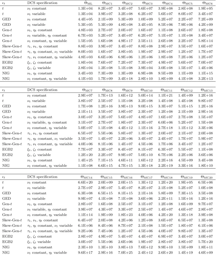
estimated in our paper. We verify condition (A.5) in Appendix.

5. Empirical results

5.1. Data

As an illustration, we use daily log-return data from the adjusted S&P 500 index

p

for

pe-riod 1950 to 2016. Some descriptive statistics of

y

are presented in Table 1. The negative

skewness estimate indicates that the mass of the distribution of

y

is concentrated on the right

side, and the high excess kurtosis estimate suggests heavy tails of

y

. The negative correlation

coefficient Corr(

y

t

,

y

) suggests that high volatility often follows significant negative returns.

We also present the partial autocorrelation function (PACF) (Hamilton 1994) up to 30 lags in

Table 1. We find significant serial correlation for the first and second lags, and we also find

sig-nificant serial correlation for the lags in multiples of around five (this indicates weekly stochastic

seasonality effects). Motivated by PACF, we use the lag order 30 for all models of location.

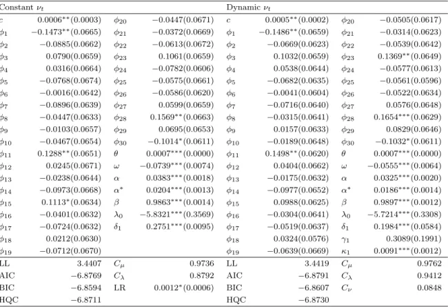
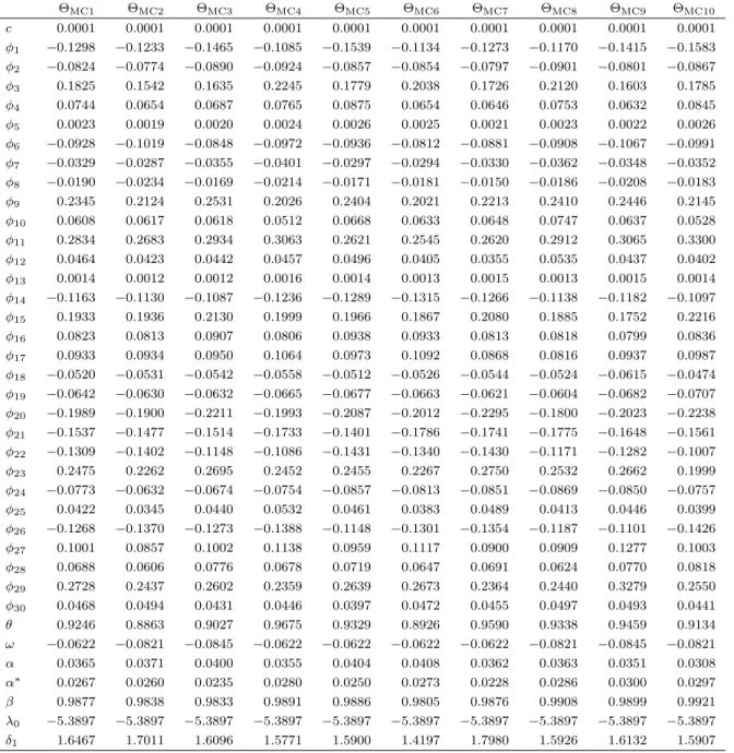
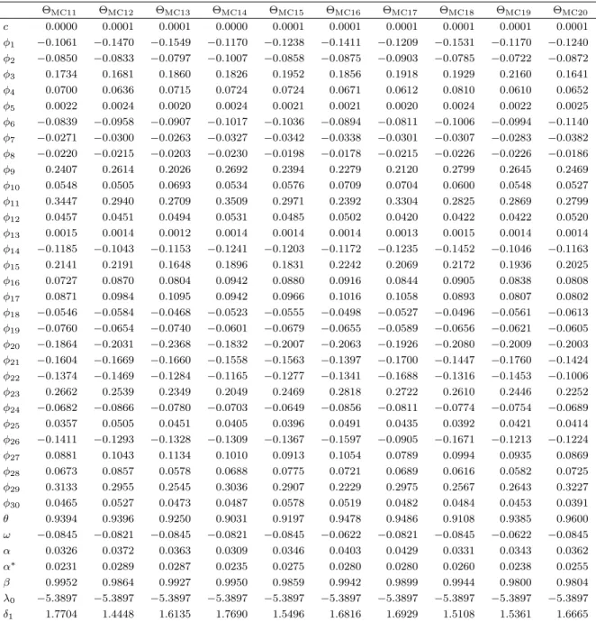
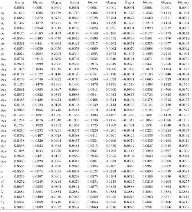
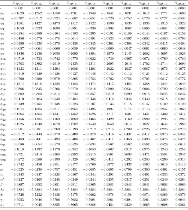
5.2. ML estimation results

In this section, we present the ML results for AR-

t

-GARCH with leverage effects (Table 2),

t

-DCS (Table 2), GED--DCS (Table 3), Gen-

t

-DCS (Table 4), Skew-Gen-

t

-DCS (Table 5),

EGB2-DCS (Table 6) and NIG-EGB2-DCS (Table 7). We compare the LL-based performance of these models

in Table 8. We present diagnostics of score functions and residuals in Table 9. We present the

evolution of scale parameters, shape parameters and volatility for all DCS models in Figs. 2 to 6.

For

t

-DCS, GED-DCS and EGB2-DCS, the ML procedure converged effectively for all

spec-ifications (i.e., all shape parameters are constant or all shape parameters are dynamic). For

Gen-

t

-DCS, three specifications were identified: (i)

ν

and

η

are constant (

ν

=

δ

and

η

=

δ

);

(ii)

ν

is dynamic (

ν

=

δ

+

γ

ν

+

κ

u

) and

η

is constant (

η

=

δ

); (iii)

ν

is constant

(

ν

=

δ

) and

η

is dynamic (

η

=

δ

+

γ

η

+

κ

u

). For Skew-Gen-

t

-DCS, three

specifi-cations were identified: (i)

τ

,

ν

and

η

are constant (

τ

=

δ

,

ν

=

δ

and

η

=

δ

); (ii) only

ν

is dynamic (

τ

=

δ

,

ν

=

δ

+

γ

ν

+

κ

u

and

η

=

δ

); (iii) only

η

is dynamic (

τ

=

δ

,

ν

=

δ

and

η

=

δ

+

γ

η

+

κ

u

). For NIG-DCS, two specifications were identified: (i)

ν

and

η

are constant (

ν

=

δ

and

η

=

δ

); (ii)

ν

is constant (

ν

=

δ

) and

η

is dynamic

(

η

=

δ

+

γ

η

+

κ

u

). Our estimation results are summarized as follows.

First, for all cases, we find that some of the

φ

parameters are significantly different from

zero. The scaling parameter of the score function with respect to location

θ

is positive and

significant for all models. For all cases, we find highly significant parameters of conditional

volatility. For almost all cases, we find that the dynamic parameters of shape (i.e.,

γ

,

γ

and

γ

) are significant and positive (the only exception is GED-DCS with dynamic

ν

, for which

γ

is not significant). We also find that the scaling parameter of the score function with respect

to the shape (i.e.,

κ

,

κ

and

κ

) is significantly different from zero for all cases (i.e., all DCS

specifications with dynamic shape are identified; Harvey 2013).

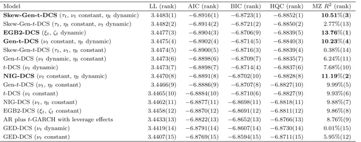
Second, we use the following model performance metrics: mean LL, mean Akaike information

criterion (AIC), mean Bayesian information criterion (BIC) and mean Hannan-Quinn criterion

(HQC) (Davidson and MacKinnon 2003). We find that the AIC-, BIC- and HQC-based

statisti-cal performances of the DCS model with dynamic shape are superior to the performance of the

DCS model with constant shape (Table 2 to 7). We also undertake a likelihood-ratio (LR) test

for non-nested models (Vuong 1989). We denote the conditional density functions of

y

of the

respectively. We define

d

= ln

f

(

y

|

y

, . . . , y

)

−

ln

g

(

y

|

y

, . . . , y

). We test whether LL of

DCS with dynamic shape is superior to that of DCS with constant shape by estimating

d

=

c

+

with OLS-HAC (ordinary least squares heteroskedasticity and autocorrelation consistent; Newey

and West 1987). If

c

is significantly positive then DCS with dynamic shape is superior to DCS

with constant shape. For almost all cases, we find that the DCS model with dynamic shape is a

superior specification (the only exception is Gen-

t

-DCS with dynamic

ν

and constant

η

). We

rank the LL-based performances of different models in Table 8.

Third, we estimate the Mincer–Zarnowitz (1969) (hereafter, MZ) regression, to rank volatility

forecast performances. For each model, we use ˆ

v

(i.e., a conditionally unbiased volatility proxy;

Patton 2011) as the dependent variable and the square of the conditional volatility (Section 3)

as the explanatory variable. Meddahi (2002) shows that the ranking of models based on the

R

_{of the MZ regression is robust to noise for conditionally unbiased volatility proxies. We}

indicate four models with the highest

R

_{by using bold numbers in Table 8. Interestingly, all}

those models have dynamics in

η

,

ξ

and

ζ

, but not in

ν

. Dynamic

ν

(i.e., dynamic heavy

tails) reduces the MZ

R

. The parameters

η

,

ξ

and

ζ

are responsible for dynamic asymmetry

and dynamic peakedness of the distribution (Fig. 1).

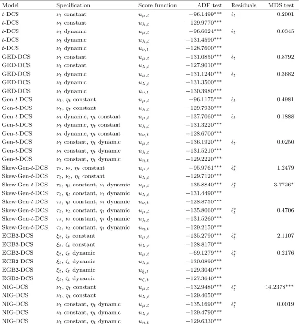
Fourth, we present the MDS test results for ˆ

and ˆ

in Table 9. For most of the cases,

we find that the null hypothesis of the MDS hypothesis is not rejected at the 10% level of

significance (the only exceptions are NIG-DCS with

ν

and

η

constant, and Skew-Gen-

t

-DCS

with

τ

,

η

constant and

ν

variable).

Fifth, the conditions for

C

,

C

and

C

are satisfied for all models (Section 4).

Sixth, Figs. 2 to 6 indicate the following: (i) the shape parameters are time-varying for all

DCS models; (ii) for the DCS models with dynamic shape, the shape parameters identify the

dates of some extreme events; (iii) the scale and shape parameters can be decomposed into a

normal risk component influenced by small or moderate changes, and an extreme component

influenced by large jumps or falls; (iv) volatility exhibits greater jumps due to extreme events

for DCS with dynamic shape than for DCS with constant shape.

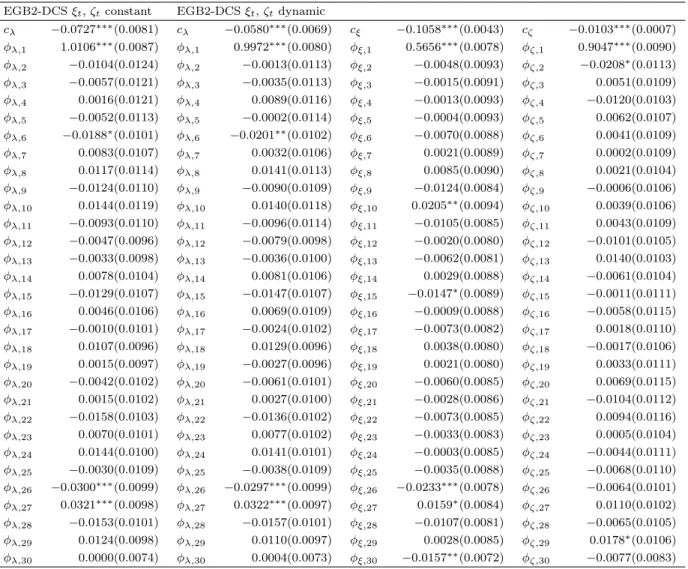
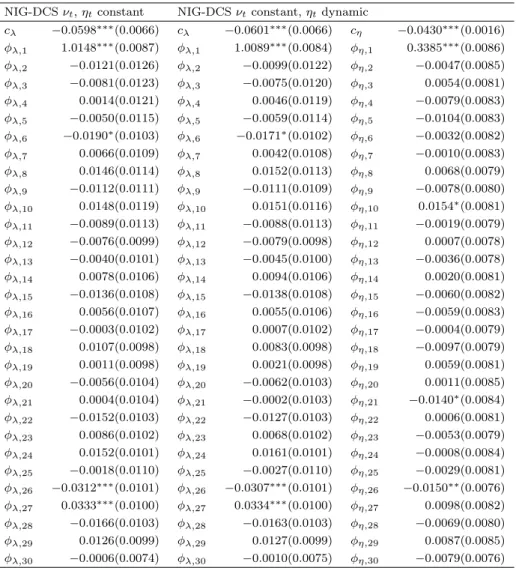
5.3. Decomposition of normal risk and extreme risk components

For the DCS models with dynamic shape, news updates volatility through

λ

and

ρ

. The

significant parameters

β

and

γ

(Tables 2 to 7), and the estimates of

λ

and

ρ

(Figs. 2 to 6)

indicate that each series can be decomposed into a normal risk component that can be related

to normal events, and an extreme risk component involving significant jumps or falls that can

be related to extreme events.

We decompose all ˆ

λ

and ˆ

ρ

series by using the equations ˆ

λ

=

c

+

P

j=1

φ

ˆ

λ

+

e

and

ˆ

ρ

=

c

+

P

j=1

φ

ρ

ˆ

+

e

, respectively. We estimate these equations by using OLS

(see the parameter estimates in the Separate Appendix). We study the consistency of OLS by

undertaking the MDS test (Escanciano and Lobato 2009) for the residuals ˆ

e

and ˆ

e

. We

find that the MDS null hypothesis of the test is never rejected (Table 10). We define the normal

risk components of

λ

and

ρ

by using the fitted values of ˆ

λ

and ˆ

ρ

, respectively. We define

the extreme risk components of

λ

and

ρ

by using the residuals ˆ

e

and ˆ

e

, respectively.

The use of 30 lags in the AR model is motivated by the PACF results of Section 5.1. The AR

model and its OLS estimation are motivated by the work of Hamilton (2017).

For each AR(30) equation, the proportion of the regression sum of squares to total sum of

squares (i.e.,

R

) is interpreted as the proportion of the dynamic parameter that corresponds to

the normal risk component (normal % in Table 10). Furthermore, for each AR(30) equation, the

proportion of the residual sum of squares to total sum of squares is interpreted as the proportion

of the dynamic parameter that corresponds to extreme risk component (extreme % in Table 10).

For the new DCS models, these results suggest that most part of

λ

is associated with the normal

risk component, and most part of

ρ

is associated with the extreme risk component. We find

that the normal component of

ρ

is significant, which motivates the use of the DCS models

with dynamic shape rather than the DCS models with constant shape.

The extreme risk component, represented by variables ˆ

e

and ˆ

e

, updates volatility

si-multaneously through

λ

and

ρ

, respectively. We study the relation between ˆ

e

and ˆ

e

for