MPRA
Munich Personal RePEc Archive
Trade costs, import penetration, and
markups
Yifan Li and Zhuang Miao
McGill University, Central University of Finance and Economics
1 April 2018
Online at
https://mpra.ub.uni-muenchen.de/91757/
Globalization, Import Penetration and Markup
∗
Yifan
Li
†Zhuang
Miao
‡JOB MARKET PAPER
Abstract
The rise of market power in recent decades has received increased attention, but the de-terminants of such a rise remain unclear. This paper studies whether and how increasing import penetration of inputs leads to a more concentrated market structure and the associ-ated rise of markups. The use of quadratic preferences in combination with the inclusion of the firm’s choice to import create a link between the use of imported inputs and markups. A reduction in importing costs induces non-importers to start importing intermediates. Yet, the effect on profits is shaped by a trade-off between the potential marginal cost ad-vantage and the fixed cost incurred from importing. As a result, only the most productive firms benefit from globalization, while existing importing firms do not fully pass through the reduction in trade costs using prices. The selection of importers, cost-savings from imported inputs and industry firm turnover jointly explain the rise of average markups in the market. Guided by this theoretical framework, we combine firm-level panel data, sector-level trade data and input-output tables to present empirical evidence on the rela-tionship between the increase in imported input penetration and the rise of market power in the US over the last four decades. Using six-digit sectors as the unit of observation, we show that imported input penetration is positively associated with the size of markups.
∗We are especially grateful to Francesco Amodio and Ngo Van Long for their advice, guidance and support. We are also thankful
to the following people for helpful comments and discussion: Francisco Alvarez-Cuadrado, Leonardo Baccini, Hassan Benchekroun, Rui Castro, Allan Collard-Wexler, Francisco Costa, Rohan Dutta, Jan Eeckhout, Christian Fons-Rosen, Amit Khandelwal, Laura Lasio, Fabian Lange, Theodore Papageorgiou, Markus Poschke, Leilei Shen, Akihiko Yanase, and all seminar participants at CIREQ Lunch Seminar Series in 2018 at McGill University, the 52nd Annual Conference of the Canadian Economics Associatoin (CEA), the 2018 Chinese Economist Society (CES) Annual China Conference, the 2018 Montreal Applied Micro PhD Day at CIRANO. Errors remain our own. The current draft is preliminary and incomplete. Please do NOT cite or distribute.
†
[email protected] (corresponding author). Department of Economics, McGill University, Leacock Building 414, 855 Sherbrooke St. West, Montreal, QC, Canada H3A 2T7.
‡
[email protected],Department of Econmics, School of International Trade and Economics, Central University of Finance and Economics, 39 South College Road, Haidian District,Beijing, P.R.China 100081
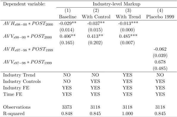
We test the model predictions on both the import decisions of heterogeneous firms and its implications for market structure. A difference-in-difference exercise that exploits China’s accession to the WTO and the use of input tariffs as a proxy for imported input penetration provide additional supporting evidence. Overall, we find that average industry markups would have been around 1.4% lower each year in the absence of imported inputs.
Keywords: globalization, import penetration, markups
1
Introduction
Discussions about the rise of market power and its macroeconomic impacts prevail in the most recent economic literature (Kwoka et al. 2015, Barkai 2016, Gutiérrez and Philippon 2016, Azar et al. 2017, Ganapati 2017, Traina 2018). The particularly evident decline in the labor share in the United States since 2000 is primarily attributed to the rise of ’superstar’ firms (Autor et al. 2017). Firm-level evidence shows that average markup has increased sharply since 1980, from 18% above marginal cost to 67% in 2014 (De Loecker and Eeckhout 2017). These studies present the rise of concentration in the market over time and have led to heated policy debates. However, the determinants of such an increase in market power remain unclear.
Importantly, another critical trend in the past several decades is globalization and the accom-panied global sourcing. Dramatic removal of trade barriers and a substantial decrease of tariffs as well as advances in communication, information, and transportation technologies have rev-olutionized how and where firms source their input for production. Indeed, there has been a substantial increase in industry openness and imports in the United States in the last few decades: the ratio of imports to GDP went up from 4.2 percent in 1960 to around 16.5 percent in 2014.1 How do firms use imported inputs in their production? How does the use of foreign imports affect industry concentration? How are markups impacted by firms’ import decisions and the change of market concentration?
Given the transformative impact of globalization, it is natural to consider the effect that import penetration may have had on the market structure and on a firm’s decisions to set the markup. The conventional wisdom underlines the intensified foreign competition as the process of glob-alization continues, which thereby alleviates the distortions associated with monopoly power. But, globalization also transforms the way firms in developed countries procure their inputs, al-though the ability of firms to select into importing might be limited to only a few firms (Antras et al. 2017). Despite the rapid expansion of global sourcing and widespread policy interest, the existing literature in trade has so far mainly focused on exporting instead of importing and has
paid relatively little attention to this facet of the interaction between imported input penetration and market concentration.
This paper aims to contribute to our understanding of the relationship between trade openness and market structure. On the one hand, import penetration increases competition from foreign producers, which implies pressure for the firms to decrease their markup. On the other hand, trade liberalization also leads to cost reduction due to improved access to imports of foreign intermediate inputs. If trade liberalization benefits only the most productive firms in each industry, the market concentration will rise as industries become increasingly dominated by large firms with high profits and low shares of labor in firm value-added and sales. To study these mechanisms, we provide a theoretical framework which relates the change in markup to the change in the extensive margin of sourcing decisions. We then look at how change in average markups is associated with imported input penetration in the process of globalization over 40 years. We combine firm-level micro panel data, sector-level trade data, and input-output tables and present empirical evidence on the relationship between the increasing trend of imported inputs penetration and the rise of market power over the last four decades. At the six-digit industry level, we find that the increase in imported input penetration is associated with increased market concentration, implying that only the most productive firms benefit from trade liberalization.
Our analysis proceeds in three steps. First, we developed a simple theoretical model that links market structure to global outsourcing. We extend Melitz and Ottaviano (2008) to include the firm’s input procurement decision and highlight the firm’s choice on importing foreign input in the spirit of Amiti et al. (2014), where the change of markup change with the extensive margin of sourcing decisions. As we work with quadratic preferences with the inclusion of the firm’s choice to import intermediate inputs, the model generates linear equations that relate changes in the variable markup with changes in the imported input penetration. A reduction in importing costs induces non-importers to start importing intermediates. Yet, the capability to profit from importing foreign inputs depends on a firm’s trade-off between the potential marginal cost advantage and the fixed cost incurred from importing. Since it requires a fixed cost of
importing to select cost-efficient intermediate inputs, the capability to benefit from the reduction of trade costs and to employ imported inputs into production depends on the level of productivity. High-productivity firms that can pay the associated fixed cost and import intermediate inputs will be thereby able to magnify their cost advantage relative to less productive firms.
Second, we illustrate some descriptive facts on rising import penetration and markups since 1970 before proceeding onto empirical analysis. We show that the ratio of imports to GDP went up from 4.2% in 1960 to around 16.5% in 2014, while the average markup increased from around 1.2 to over 1.6 in the same period. Import penetration has an ambiguous relationship with markup. Standard trade theory would predict reduced markup due to more imported output competition. But, if the market is imperfectly competitive, a reduction in trade costs due to globalization will have heterogeneous impacts on the markup of firms that import inputs and firms that rely only on domestic input. Therefore we distinguish import penetration in output and input and measure them separately. Indeed, when we look at imported input penetration, we find a strong correlation between the rise of imported input penetration ratio at the level of 2-digit sector weighted average markup based on firm-level sales, while the overall import penetration ratio shows an ambiguous relationship with the change of markup. This is because the import penetration ratio mixed the effect of competition from the final goods with the effect of employment of cheaper/better inputs on market structure. Making use of imported inputs contributes to the decrease in the firm’s marginal cost and increases the firm’s potential of higher markup. But it may require some level of firm ability to take advantage of imported inputs.
Third, we present empirical evidence on the relationship between the rise of market power and the increase in imported inputs penetration over the last four decades. We use firm-level panel data that contain critical balance-sheet variables such as sales, the number of employees and capital for production function estimation from WRDS-Compustat Database. By applying the production-based approach (De Loecker et al. 2016), we estimate markups at firm level from 1972 to 2014. We then measure direct import penetration level from industry-level trade data from the United States import and export Data of the Center for International Data, UN COMTRADE, and USA Trade Online. Combining input-output benchmark table at the 6-digit industry level
from the Bureau of Economic Analysis (BEA), we measure indirect intermediates import pene-tration by weighting the direct import penepene-tration ratio with the degree of interdependence of each industry pair. We find that a 10% increase in the rise of imported input penetration is associated with a 0.2% increase in market concentration, implying that only the most productive firms benefit from trade liberalization. We further test our predictions of heterogeneous firms’ decisions on intermediates importing and the implications on the market structure using out-put and inout-put tariffs as proxies for import: a 10 percent increase of inout-put penetration induces roughly 1.2 percent increase of markup on average. This finding is robust to different model specifications at both the firm and industry levels. It also survives from various concerns of the model including alternative markup measure, alternative benchmark weighting in accounting for input penetration, and the use of derived input tariff as a proxy for input penetration. We also applied a difference-in-difference approach taking China’s accession into the WTO as a trade shock to provide additional support to our main predictions.
This paper explores the mechanism that links the globalization process to the trend of rising markups over the last four decades. The contributions of this paper are twofold. First, we construct a theoretical model that links the rise of the input imports and the increase of average markups, and also distinguishes the changes of the market structures during this process, i.e., the entry-exit decisions, outsourcing decisions, and price strategies made by heterogeneous firms. Second, we provide empirical evidence that supports these predictions and the mechanisms identified in theory. A difference-in-difference exercise that exploits China’s accession to the WTO and the use of input tariffs as a proxy for imported input penetration provide additional supporting evidence to the theory.
Our paper contributes to several strands of the literature. We add to the vibrant empirical research that looks at the ambiguous effects of trade liberalization on markups (Burstein and Gopinath 2014). There is empirical evidence of reduction of markups due to more competition following dramatic trade liberalization for some countries. For example, Badinger (2007) finds a decrease of markups in aggregate manufacturing sectors following the EU’s Single Market Programme. Some literature discovers that trade liberalization of intermediates inputs may lead
to markup increase due to various reasons. Ludema and Yu (2016) explain the incomplete pass-through of foreign tariff reductions with firms’ quality-upgrading strategies, which are estimated to be greater for high productivity firms. Amiti et al. (2014) develop an oligopoly framework with variable markups and imported inputs, and find that firms with top import shares have low exchange rate pass-through. Brandt et al. (2017) find that cuts in output tariffs reduce markups while cuts in input tariffs raise both markups and productivity by examining China’s WTO accession and the performance of Chinese manufacturing firms.2
These case studies focus on the impacts of striking shocks such as trade liberalizations for a relatively short period. They link markup variation exclusively to a market share of the firm, neglecting the effect that exogenous change of variable cost has on industry reallocation in the long run. Instead, our paper looks at the impact on the industry that the broad process of globalization brings over 40 years, which combines short-run effects of trade cost reduction on marginal cost and competition with the impact on industry reallocation in the relative long term.
Our theoretical framework is closely related to and is built upon Melitz and Ottaviano (2008) and Halpern et al. (2015). Melitz and Ottaviano (2008) develop a monopolistic competition model of trade with firm heterogeneity which has been a workhorse model that predicts intra-industry reallocation between firms with different mark-ups following trade liberalization. Halpern et al. (2015) estimate the productivity gain from the improved access to foreign input. They assume a constant elasticity of substitution (CES) utility function and provide a static model of industry equilibrium where firms use both domestic and imported intermediates goods for production. However, CES utility directly implies constant markup and make it unsatisfactory to analyze variable markup changes concerning aggregate shocks. We instead employ the linear demand system as in Melitz and Ottaviano (2008) and trace in detail how imported input penetration plays a role in the pricing of firms that have better ability to utilize sourcing opportunities. If firm heterogeneity interacts with fixed sourcing costs, the firm’s decision to import from one
2Other case studies include Fan et al. (2018) for China, De Loecker et al. (2016) for India, Altomonte and
Barattieri (2015) for Italy, Moreno and Rodríguez (2011) for Spain, Konings et al. (2005) for Bulgaria and Romania and Harrison (1994) for Cote d’Ivoire.
market will also affect market structure. In our model, a reduction in global sourcing costs induces a firm to increase imports of low-cost input and to increase the markup. But the access to foreign inputs is restricted to the firms that can pay the fixed importing cost and use imported intermediates. Our model predicts that, as the cost of importing decreases, existing importing firms will import more foreign intermediate varieties, leading to even better advantages in both product quality and production cost. These two effects will magnify existing strengths that more productive firms have relative to less productive firms. This, in turn, implies that trade liberalization has asymmetric impacts on the market share of existing market players.
Our paper also relates to the literature that looks at the global trend of market power and its consequences. De Loecker and Eeckhout (2018) document the rising trend of global market power. While it is more salient in the developed world than in the emerging areas, the average global markup increased from 1.1 to 1.6 between 1980 and 2016. For the U.S in particular, the average mark-up has been increasing dramatically since the 1980s, and it is believed to be associated with several other macroeconomic trends such as the decline in labor and capital share, the decrease of low skill labor wage, and the slow down in aggregate output (De Loecker and Eeckhout 2017). Autor et al. (2017) reassess the secular trend of labor share through micro panel data since 1982 and interpret the fall in the labor share to be the result of the rise of “superstar firms” that dominate the market with high profits and low share of labor in firm value-added and sales. They also notice the potential role that globalization and technological changes might have played but are skeptical as the fall in labor’s share also appears in non-traded sectors like retail and wholesale, not just in non-traded industries like manufacturing. There is other circumstantial evidence in this story of rising market power.3 A paper that is closely
related to ours is that of Elsby et al. (2013), who consider the potential impact consider the possible effects of globalization and rising imports on the decline of labor share. They provide a set of simple cross-industry regressions and graphs and show that the variation in the change in import exposure explains 22 percent of the cross-industry variation in payroll-share changes.
3For example, increased profits (Barkai 2016), decreased investment(Gutiérrez and Philippon 2016), decreased
wages in concentrated markets (Azar et al. 2017), weakened antitrust enforcement (Kwoka et al. 2015), and restricted output (Ganapati 2017).
While these studies try to link the rise of market power of superstar firms as the cause for the decline of labor share, our purpose is to propose a mechanism that drives this rising market concentration and to illustrate how less-frictional international trade enables more efficient firms to be rewarded with higher market shares today than in the past. Our paper looks not only at the direct impact, i.e., the substitution effect, which depresses the labor share of domestic income and reduces the marginal cost of firms that employ cheap foreign inputs, but also the indirect impact, which changes the market structure to be more concentrated as only some firms can pay the fixed cost and utilize global opportunities. We also provide direct empirical evidence of these mechanisms.
Finally, our paper complements a large body of literature that evaluates welfare gains from trade by estimating its impact on markup heterogeneity and allocative efficiency. Epifani and Gancia (2011) document several stylized facts about markup dispersion across industries over time and in a relationship with exposure to trade. They provide an oligopoly framework with CES utility and find that markup heterogeneity entails significant costs and that asymmetric trade liberalization may reduce welfare when there exists restricted entry. Feenstra and Wein-stein (2017) consider symmetric translog preferences and structurally estimate the welfare gain of globalization into variety-increase and markup-decline channels. There are two critical differ-ences between the theoretical framework in these papers and the model we present here. First, our paper adopts monopolistic competition with linear demand system which allows markup variability to depend not only on market share but also on imported input substitution and product/industry characteristics. Second, in our framework, a change in the trade costs in-duces marginal cost change directly and inin-duces price change indirectly through both general equilibrium effects (the number of active firms) that shift or rotate the firm’s demand curve.
The rest of the paper is organized as follows. Section 2 presents a general theoretical framework that encompasses monopolistic competition and variable markup to examine the impact of trade cost reductions on firms’ markups and associated intra-industry reallocation. Section 3 describes the datasets and measurements used. Section 4 presents our econometric specifications and report the main results, followed by an interpretation of the underlying mechanisms. Section 5
provides a series of robustness checks. The last section concludes.
2
Theoretical Framework
In this section, we develop our theoretical framework of global sourcing and markup. Our model is based on an extension of Melitz and Ottaviano (2008). Building upon Halpern et al. (2015), we incorporate Amiti et al. (2014)’s way to model the firm’s cost structure and its choice to import intermediate inputs. We extend the model by relating the option of importing to productivity and analyze its comparative statistics. In sections below, we present the model and derive equilibrium prices, sourcing strategies, marginal cost, and markups. Since our model is similar to Amiti et al. (2014), we relegate most of the derivations to the Appendix and examine here in more detail the impact of increasing import penetration on markups.
2.1
Consumers
Preferences are defined over a continuum of differentiated varieties indexed by i ∈ Ω , and a homogeneous good chose as numeraire. As in Melitz and Ottaviano (2008), consumers share the same quasi-linear utility function given by
U =q0c+α ˆ i∈Ω qcidi− 1 2γ ˆ i∈Ω (qic)2di− 1 2η ˆ qicdi !2 (1) where qc
0 and qic represent the quantities of the numeraire good and the differentiated variety
i respectively. The demand parameters α, η, and γ are all positive. The parameters α and η index the substitution pattern between the differentiated varieties and the numeraire good, and the level of competition intensity among differentiated varieties. The parameter γ indexes the decreasing rate of the marginal utility for each variety. Given the price for varietyi , consumers
decide their quantity demand as followings. qi ≡Lqic= αL ηN +γ − L γpi+ ηN ηN +γ L γ ¯ P (2)
whereLdenotes the population of the economy,N measures the mass of varieties in Ω (which is also the number of active firms) and ¯P = N1 ´i∈Ω∗pidi is the average price of all varieties existing
in the market. The set Ω∗ is the collection of the varieties that exist in the market. In other words, the variety which belongs to the set Ω∗ must satisfy
pi ≤
1
ηN +γ(γα+ηN ¯
P)≡pmax (3)
This inequality suggests that all firms’ prices will be up-bounded by the price level charged by the lowest productivity firm. This is because low-productivity firms need to charge relatively high level of prices in order to cover their high variable cost. Among the surviving firms, the demand is limited to the price that the lowest productivity firm charges.
2.2
Producers
For simplicity, we assume that final-good varieties are prohibitively costly to trade across bor-ders. We do this in order to highlight the trade of intermediate input as the relevant mechanism.4
Similar to Amiti et al. (2014), we model the cost structure of the firm and its choice to im-port intermediate inputs. Consider firm i, indexed by its productivity Ai, uses labor Zi and a
composite intermediate input Xi to produce output Yi according to the production function:
Yi =AiXiφZi1−φ (4)
4The model could be extended to accommodate trading of final goods and the extensive margins of both
The composite intermediate inputXi consists of two types of intermediate goods, one of which
could be purchased either locally or imported from the foreign market and the other one of which could only be procured domestically. Di represents the quantity of the domestic-specific
input which can only be purchased domestically, andMi represents the amount of intermediate
inputs which could be sourced from either the domestic or the foreign markets. Let ξ be the elasticity of substitution betweenDi and Mi .
Xi = " D ξ 1+ξ i +aM ξ 1+ξ i #1+ξξ (5)
Intuitively, a measures the productivity advantage of the foreign variety. Although production is still possible without the use of imported inputs, imported inputs are useful due to (i) their potential productivity advantagea, and (ii) the love-of-variety feature of the production function. The prices of imported inputs and domestic inputs are denoted byPM andPD respectively, and
we assume the firms are price takers in these input markets.
For each imported intermediate good, firm i must incur a fixed cost fi(Ai), which depends on
firm productivityAi. Examples for the fixed importing costs include the information gathering
and search cost, management cost, cost for an import permit, and the production adjustment for various inputs. We believe the high productivity firms pursue cost advantage in both the production and importing processes. For example, the high productivity firms hire the high productivity workers who will lower the management cost. They are more likely to export to more markets and pursue widely international connections, which will lower the search cost. In section 2.5, we relax the assumption on the dependence of the fixed cost while assuming a complementary form of the production function. The main predictions of that model are consistent with the one with the fixed cost endogenous to the productivity.
The presence of fixed costs have been founded empirically and have been widely assumed (Amiti et al. 2014; Antras et al. (2017); Gopinath and Neiman (2014); Halpern et al. (2015)). Here we further assume that the fixed sourcing cost a firm has to pay to start importing intermediate inputs is decreasing with productivity. If we think of the fixed cost as the searching and
informa-tion cost a firm pays to find the most cost-efficient external input supplier, then it is reasonable to believe that high-productivity firms are likely to find the desired trading partner easier.5
Following this setting, we compute the variable cost index for importers and non-importers as follows Vi = 1 + τ mPM f a 1 1+ξ 1+ξ importer " 1 + (PM d) 1 1+ξ #1+ξ non−importer (6)
where PM f and PM d are the prices for the foreign and domestic intermediates respectively; τm
captures the trade cost of purchasing the foreign intermediates.
The marginal cost of firmi is equal to:
ci =ςϕi W 1−φ !1−φ Vi φ !φ =ςϕiV φ i − D (7)
whereW measures the domestic labor cost, thus −
D≡(1W−φ)1−φ(1
φ)
φ is a common cost factor for
both importers and non-importers. ϕi is the inverse productivity of firm i, i.e. Ai = ςϕ1i, where
ς is a parameter. ϕi is assumed to follow a Pareto distribution, i.e. ϕ∼
ϕ−ϕ ϕ−ϕ k with support h ϕ, ϕi. 6
Notice that the term D− is identical across all the firms. Moreover, firms only differ in their productivity levels and the termVi, depending on how much the foreign inputs they use.
In a closed economy, firm i only sources from the domestic market, so the profit maximization problem is:
M axpiπ
D = (p
i−ci)∗qi
5Alternatively, this assumption could be replaced by a quantitative constrain on the relative scale of fixed
cost and net profit of being an importer. Moreover, we relax this assumption and consider a constant fixed cost case in the following section 2.5.2.
6Recall that the productivity level for firmiis denoted asAi, thus ςϕ
i= A1
Profit maximization implies the following results: piD = 12(ci+cd) µiD = (ci2+ccd) i qiD = L(cd −ci) 2γ riD = L(cd −ci)(cd+ci) 4γ πiD = L(cd −ci)2 4γ (8)
where pi(cd) = pmax =12(cmax+pmax), therefore, pmax = cd, and cd is the cut-off cost value for
the firms to be able to survive in the market with their exact variable cost, i.e, all the firms whose variable cost is higher than this value will not be able to survive in the market. To simplify our analysis, we assume the firms’ entry decision and the reveal of the productivity information take place during the same period.
Assume the firm’s variable cost c is drawn from a known distribution G(c) with support [c, c].
7 The cost (productivity) cut-off is thus determined by the free-entry condition:
cd
ˆ
c
π(ci)dG(c) =fE (9)
The mass of surviving firms is determined usingcd and the zero demand price condition:
cd= γα+ηNP¯ ηN +γ (10) which implies N = γ η α−cd cd−P¯ (11)
and the mass of entrants
NE =
N G(cd)
(12)
7Under the case of closed economy, the variable c follows the same type of distribution as the inverse
From which it follows ¯ P = ˆ ω∈Ω p(ω)dω= cd ˆ c ci+cd 2 dG(ci)/G(cd) (13)
2.3
The Equilibrium
2.3.1 Determination of importing productivity cutoff
For simplicity, we keep the number of entrantsNE and the productivity distribution G(.) fixed.
The number of survived firms is thusN =NEG(ϕd), whereϕdis the cut-off value of productivity,
i.e. cd = ςϕdV φ i
−
D. Recall that the inverse productivity is assumed to be drawn from a Pareto distribution, ϕ ∼
ϕ−ϕ ϕ−ϕ
k
with support hϕ, ϕi. Following Antras et al. (2017), we assume that importing intermediate from the foreign market requires a fixed cost fm , whose value
is identical to all firms. Firm i decides whether to import the intermediates based on the expected profits it faces. As we assume that the firm only imports one type of input from one foreign country, the index Viφ should be identical across all importing firms, i.e. Viφ =Vφ. For
simplicity, we further define Ψ = Ψi ≡ ςViφ
−
D for importing firms (where − D ≡ (1W−φ)1−φ(1 φ) φ) and normalize ςViφ −
D = 1 for all non-importing firms. The firm will import intermediates if H(ϕi)≡π(ϕi|importer)−π(ϕi|non−importer)> fm, whereπ(ϕi|importer) =
pfi −ϕiΨ
∗qfi with Ψ<1 and π(ϕi|non−importer) =
pd i −ϕi ∗qd i.
This mechanism is presented in the illustrative Figure 1. The unit cost savings that importing brings is constant. When a firm is the most productive (inverse productivity is 0), it can charge highest price, sell most products and get highest profits. Importing foreign inputs brings no change to its unit cost due to the cost structure, so to the price and quantity. Thus the profit difference curve cross the origin. As a firm becomes less productive, it prices relatively lower, sell less and profit decreases. But at the same time importing starts to bring in advantage because it decrease unit cost by a certain amount, counteracting the decrease in productivity, and brings positive profit difference. Until reaching a point where the negative effect that the decreases in productivity brings on profit, exceeds the positive effects that the constant unit cost savings
that importing brings on profits. And the profit difference curve starts to become downward sloping.
Proposition 1. Given the highest inverse productivity of the survived firms in the market and the following assumptions. (i) Importing fixed cost fm is identical to all firms, and (ii) the
fixed cost satisfies the conditions ϕ > 4γfm(1+Ψ)
L(1−Ψ) and ϕ < 2 1−Ψ
q
γfm
L , then there exists an unique
solution ϕm which solves H(ϕm) = 0 in the definition range ϕm ∈
h
ϕ, ϕi, and it follows that
H(ϕ)≥0 for ϕ < ϕm and H(ϕ)<0 for ϕ > ϕm.
Proposition 1 implies that only high productivity firms make importing, and the firms whose inverse productivity is higher than a critical value, then they won’t make importing. Specifically, this critic value is solved as:
ϕm = ϕd+ r ϕ2 d− 4γfm(1+Ψ) L(1−Ψ) 1 + Ψ (14)
When the value ofϕm is less thanϕd, for the firms whose inverse productivity is lower than ϕm
will choose to import the inputs, and the firms with higher inverse productivity will choose to use domestic inputs only. Ifϕm ≥ϕd, then all the firms in the market will not choose to import
the intermediate inputs.
2.3.2 Determination of the number of active firms and productivity cut-off
In the open economy case, equation (13) becomes:
¯ P = ϕm ˆ ϕ ϕΨ +ϕd 2 ! dG(ϕ)/G(ϕd) + ϕd ˆ ϕm ϕ+ϕ d 2 dG(ϕ)/G(ϕd) (15) Asϕ∼ ϕ−ϕ ϕ−ϕ k
¯ P = ϕm ˆ ϕ k ϕΨ +ϕd 2 ! ϕ−ϕ ϕd−ϕ !k−1 1 ϕd−ϕ ! dϕ+ ϕd ˆ ϕm k ϕ+ϕ d 2 ϕ−ϕ ϕd−ϕ !k−1 1 ϕd−ϕ ! dϕ (16)
The example with the uniform distribution function is solved as:
¯ P = 4 ϕd−ϕ ! h 3ϕ2d−(1−Ψ)ϕ2m−Ψϕ+ 2ϕd ϕi (17)
Then the firm number is solved as:
N = γ η α−ϕd ϕd− 4 ϕd−ϕ h 3ϕ2 d−(1−Ψ)ϕ2m− Ψϕ+ 2ϕd ϕi (18)
Equation (18) shows that the number of survived firmsN is negatively correlated with the cut-off value ϕd. Recall from equation (12) that we have another relation between N and ϕd , i.e.
NE = G(Nϕ
d), which indicates a positive relation between N and ϕd when the entrant massNE is
fixed in short-run. Equations (12), (14), and (18) uniquely determine the inverse productivity cut-offϕdand firm number N , which is illustrated in Figure 3. The positive relation betweenN
and ϕd (equation (12)) represented by curve S suggests that the market will be able to support
more active firms when the productivity cut-off is low (high ϕd), while the negative relation
between N and ϕd (equation (18)) represented by curve D implies that only a limited number
of firms could survive in the market due to high choke price induced by low productivity cut-off (highϕd).
2.4
The Impact of Globalization
The process of globalization suggests a continuous reduction of trade costs between countries. According to Equation (14), a reduction of variable trade cost will induce a lower price level of intermediate input Ψ, making it more profitable for a firm to engage in intermediate input
trading. Equation (14) shows that the inverse productivity cut-off to import foreign inputϕmwill
be higher. This implies that there are more firms engage in importing cost-efficient intermediate input. This is illustrated in Figure 2, where the expected profit curve moves outward when there is a reduction in trade cost, leading to a higher inverse productivity cut-off value to become an importing firm.
Equations (18) and (12) determine the equilibrium level of N and ϕd as shown in Figure 3.
It is clear that when the trade cost Vφ decreases, the curve D1 shifts downwards while the S
curve remains unchanged. This is because the relation between N and ϕd in Equation (12) is
uncorrelated with trade cost this is is not the case for Equation (18). Solving the new equilibrium gives a lower level of N and ϕd as shown in Figure 4. This indicates that the number of active
firms in the market shrinks following the reduction of trade costs. Moreover, a smaller ϕd
suggests that the productivity cut-off level to survive in the market also increases.
From simple differentiation of equations (14), (18) and (12) it follows that:8
Proposition 2. A decrease in variable trade cost τ induces the number of active firms in the marketN and the inverse productivity cut-off to survive ϕd to decrease, i.e.∂N∂Ψ >0and ∂ϕ∂Ψd >0;
furthermore, if the change of cut-off value is small enough, i.e. ∂ϕd
∂(1+Ψ) 1+Ψ
ϕd <1, in response to a
reduction of the trade cost τ the importing critical value ϕm will increase. 9
The average markup across all firms that survive is derived as:10
¯ µ= ϕm ˆ ϕ k ϕΨ +ϕd 2ϕΨ ! ϕ−ϕ ϕd−ϕ !k−1 1 ϕd−ϕ ! dϕ+ ϕd ˆ ϕm k ϕ+ϕd 2ϕ ! ϕ−ϕ ϕd−ϕ !k−1 1 ϕd−ϕ ! dϕ (19)
An example with the uniform distribution is written as:
8The details of the derivation are presented in Appendix A2. 9The condition ∂ϕd
∂Ψ <
4γκΨ+ϕdL(1−Ψ)2(1+Ψ)
L(1−Ψ)2(1+Ψ) is easy to satisfy if the value of Ψ is closed to one.
¯ µ= ϕd 2ϕd−ϕ | {z } (1) 1 Ψln ϕm ϕ | {z } (2) +lnϕd ϕm | {z } (3) − 1 2ϕ (20)
wherek is the parameter for the distribution of inverse productivity; ϕd is the surviving cut-off
value of the inverse productivity; ϕm is the critical value of the inverse productivity to import;
and Ψ captures the variable cost of importing the inputs.
Combining the latter with equation (14), we observe that if ∂ϕd
∂(1+Ψ) 1+Ψ
ϕd < 1 , then
∂ϕm
∂Ψ < 0,
which means that when importing cost decreases, more firms will use the imported inputs. This condition also implies that the average markup ¯µ decreases in the importing cost Ψ, i.e,
∂µ¯
∂Ψ < 0. In other words, a lower importing intermediate price index leads to a higher average
markup. Specifically, based on the equation (20), we observe that the the link between trade cost and average markup materializes via two different channels. First, there is a higher share of high productivity firms. The first term of (20) captures the exit of low productivity firms and then the sales reallocates to the high productivity firms with high markup. The second term of (20) captures the fact that in response to a reduction of importing cost, the importing firms will obtain higher markup, wherelnϕm
ϕ indexes the share of the importing firms out of all
survived firms. The third term measures the increase of market competition due to that the importing firms charge a lower price in response to a reduction of input price. When the first and second effects dominate the third effect, then the average markup will increase in response to the reduction of importing cost.
Proposition 3. In response to a reduction of the trade cost, if the change of the surviving cut-off value is small enough, i.e. ∂ϕd
∂Ψ Ψ
ϕd < lnϕ, the industry’s average markup µ¯ will increase. This is
2.5
Extensions
This section completes our theoretical framework by altering a few dimensions of our modeling setup and see how the results change. First, we allow the entry mass to be endogenously determined by the free entry condition and discuss the conditions under which that our model main predictions remain. Second, we turn the fixed sourcing costs that are previously increasing in the firm’s inverse productivity into a constant independent one, and we show that the relevant expressions would all be very similar. Third, to highlight the importance of importing, we have assumed that final goods cannot be traded across borders. We relax this assumption and study the joint determination of the extensive margins of both exports and imports.
2.5.1 Endogenous Number of Entrants
In the model so far we kept the entry mass NE constant. It could be endogenously determined
by the entry condition and supply of the entry firms, i.e.
´ϕm ϕ L − D 2 (ϕd−Ψϕ)2 4γ dG(ϕ) + ´ϕd ϕm L − D 2 (ϕd−ϕ)2 4γ dG(ϕ) =fE N =NEG(ϕd) (21)
Both equations together determine the supply side of the entry firms. From equation (14), we know that ϕm is an increasing function of ϕd, given the value of Ψ. In this way, the value of
ϕd is determined by the entry cost fE and independent of the firm numberN. In this case, the
curve which illustrates the supply side of the entry firms is drawn as a horizontal line in the Figure 6 below (the curve S1). It is easy to prove that when the trade cost Ψ decreases, the
demand curve D1 shifts down to the position of the curve D2, and the supply curve S1 shifts
down to the position of the curveS2. In this case, the inverse productivityϕddecreases but the
change in the cut-off value for the firm number N depend on the relative associated change of both the supply and demand curve. Although we are not able to make quantitative statement
on the changes of the importing critical value ϕm in this case, it is qualitatively clear that our
min prediction on average markup ¯M remains as long as the firm entry incurred by the rise of imported input penetration remains in a relatively small scale over the observation period.
2.5.2 Independent Fixed Sourcing Cost
One might be concerned with the seemingly strong assumption that the fixed sourcing cost a firm has to pay to start importing intermediate inputs is decreasing with productivity, though it is well-justified by the fact that the searching and information cost it incurs to find the most cost-efficient trading partner is likely to fall with productivity. To address this issue, we relax this assumption and assume an independent fixed sourcing cost. We make the following assumptions on the production function. It requires two types of inputs in the production, i.e., labor and intermediate input. One unit of composite intermediate input can be transformed into φ units of the final output. It requires at least A1
i unites of labors to complete the transformation of one
unit of output, where the parameter Ai captures the labor productivity for the firm i.
Yi =min{AiLi, φXi} (22)
The marginal cost of firmi is computed as:
ci =ϕiW +φVi
whereVi and W are price for the intermediate input and wage of the labor respectively;ς and φ
are parameters with given values; and ϕi is inverse productivity of firm i, which is assumed to
follow a Pareto distribution, i.e. Ai = ςϕ1i and ϕ∼
ϕ
ϕ
k
with support [0, ϕ]. We can then prove the following lemma:
Lemma 1. When the importing fixed cost is small enough, i.e. fm <
(W ϕd−φΨ+12 )
a ϕm ∈[0, ϕd] which solves H(ϕm) = 0 ; and H(ϕ)≥0 for ϕ < ϕm and H(ϕ)<0 for ϕ > ϕm.
In this case, the survived firm who has lowest productivity won’t choose to import the interme-diates.
Specifically, the critical value ϕm is given by:
ϕm= 1 W " W ϕd+ 1−Ψ 2 − 2Υ fm L(1−Ψ) # (23)
According to Lemma 1 , the firms whose inverse productivity is lower than ϕm will choose to
import and the firms with higher inverse productivity will choose to use domestic inputs only.
Similar derivations give the average markup as:11
¯ µ= ϕˆm 0 " W ϕ+ Ψ +W ϕd+ 1 2 (W ϕ+ Ψ) # dG(ϕ)/G(ϕd) + ϕd ˆ ϕm " W ϕ+ 2 +W ϕd 2 (W ϕ+ 1) # dG(ϕ)/G(ϕd) (24)
Assuming that the inverse productivity follows uniform distribution, i.e. k = 1 and ¯ϕ= 1, the average markup across all firms that survive is derived as:
¯ µ= 1 2 1 + W ϕd+ 1 W ϕd | {z } (1) ln W ϕm+ Ψ Ψ (W ϕm+ 1) | {z } (2) + W ϕd+ 1 W ϕd ! ln(W ϕd+ 1) | {z } (3) (25)
It follows that the average markup ¯µ increases in the importing critical value ϕm. Similar to
the results in the case of Cobb-Douglous productivity function, we observe two channels for the rise of the average markup in reacting to the reduction of Ψ, i.e. the reallocation effect and cost reduction effects. Term (1) of 25 captures the reallocation effect such that lowering importing cost reduces the surviving cut-off ϕd, which increases the proportion of high productivity firms
in the market. Term (2) reveals the fact that lower importing cost reduces the variable cost of the importing firms directly, which enhances the competition capacity of these firms. Term (3) increases in ϕd, which reveals that the firms that never import inputs will face higher intense
of market competition after the importing cost reduces, and thus their markups will be lower than before. When the effects of terms (1) and (2) dominates the effect of term (3), the average markup will increase in react to a reduction of the importing cost. As a result, a reduction in variable trade costs increases the average markup due to these two effects. Next, we will show that in response to a reduction of importing cost, the average markup will increase when some conditions satisfy. Recall that from 10, the change of ϕd is very small in response to the
varying of importing cost when the parameter η is small enough. If we set η = 0, ϕd will be
constant in the importing cost Ψ. Given this property, when the importing cost Ψ decreases, the importing critical value ϕm will increase according to 23. That means more firms will enter
the international input market. Given all these properties, we observe that, terms (1) and (2) of 25 are constant in Ψ while term (2) decreases in Ψ. In this case, we will observe an increase of average markup in response to a reduction of importing cost Ψ. Actually, when the parameter η is small enough (not necessary to be zero), the change of term (3) will be very small and the average markup still decreases in Ψ .
3
Data and measurement
Our theoretical framework shows that a decrease in trade cost and the associated rise in input import penetration is associated with a surge in the markup. It is due to both a cost reduction and reallocation effect. The remainder of the paper aims to find empirical evidence that supports this claim. To uncover the relationship between input import penetration and markups, we use Compustat data of US public firms to generate markup, and we combine US trade data and Input-Output tables to test the impacts of import penetration on markups. The empirical exercise is based on three main types of data for the empirical analysis: firm’s balance-sheet
data, trade data, and input-output tables at detailed commodity level.
3.1
Firm Balance-Sheet Data
We use Compustat (North America) Fundamental Annual database to derive firm-level balance sheet information. Compustat has variables that are needed for production function estimation including annual sales, wages, capital stock, as well as the labor of all the US publicly traded firms available from 1950 to 2014 in Wharton Research Data Services (WRDS). We restrict the sample as follows: First, we only consider and identify firms incorporated in the United States based on Stock Exchange Code (EXCH) and Foreign Incorporation Code (FIC); Second, we exclude observations with obviously mis-measured variables of interests, such as negative sales or employment. The final sample counts 504,319 firms-year observations covering the years from 1972 to 2014. The common GDP deflator comes from the Bureau of Economic Analysis’s National Income and Product Accounts (NIPA) tables of the United States. Therefore we obtain firm-level markup by applying the so-called cost-based production approach as in De Loecker and Warzynski (2012).
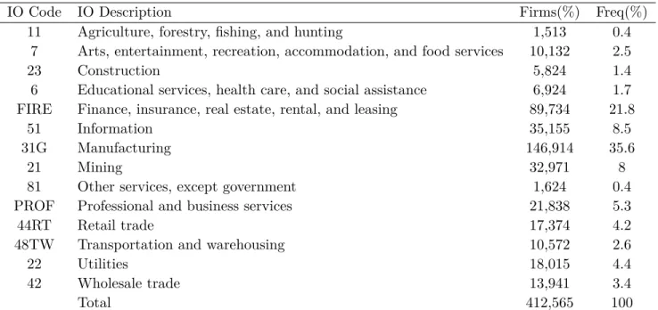
Constrained by the data availability of import penetration measures, we focus on the sample from 1972 to 2014, that we match with industrial level import penetration ratios in the firm-level regression. It reduces our sample to 412,565 firms-year observations with an average of 9,822 firm-level observations per year. Compustat assigns each firm a North American Industry Classification System (NAICS) 2012 6-digit sector code based on the firm’s operation reported as required by Financial Accounting Standards Board (FASB). The 2012 NAICS codes have 1,065 disaggregate industries. To match it with the industrial classification in the Input-Output table, we first converted the different versions of NAICS codes to the 2007 version and then assigned each 2007 NAICS code with one of the 389 6-digit IO industries used in the Input-Output table from Bureau of Economic Analysis (BEA). Table 2 shows the IO industrial distribution of the firm-year observations at the most aggregate level between 1972 to 2014. While Compustat only
includes publicly traded companies, our sample covers firms across most of the industries and matches closely with the industrial distribution across the economy. A large portion of firms is in the Manufacturing and Finance sector, accounting for 35.5% and 21.8% of the observations respectively in the sample. We are interested in how imported inputs penetration is related to markup at the firm level, but Compustat does not contain information on how much each firm employ foreign inputs. Therefore in the industry-level regression, we compute the sales-weighted markup at the 6-digit BEA I-O industry level to match with industry-level import penetration measures.
3.2
Markup Estimation
Defined as the ratio of price over marginal cost, markups can be estimated by a few different methods prevailing in the field of empirical industrial organization. As detailed data on price and marginal cost data is usually unavailable, markup estimation depends on the granularity of the available data and the choice of assumptions. On the one hand, the “demand-based” estimation requires assumptions on the form of demand function and market structure, therefore marginal cost and markups are estimated with the associated demand elasticity and firms’ optimal pricing behavior as in Bresnahan (1982) and Berry et al. (1995). On the other hand, the “production-based” method proposed in De Loecker and Warzynski (2012) builds upon the insight of Hall (1988) where markups are inferred by estimating the production function with assumptions on the firms’ optimal input choice from total cost minimization. Markup is then derived as the product of the input revenue share and output elasticity of any chosen variable input. Intuitively, it is measured as technology-adjusted cost share. As the input cost shares are often available in the accounting data, it is easy to estimate markup by having an estimate of the input elasticity. The input elasticity is estimated using various production function estimation methods including OLS, Olley-Pakes, and Levin-Petrin methods. And our baseline results are based on Olley-Pakes method.
We adopt the “production-based” method in our markup estimation for several reasons. First, one of our model prediction is that imported input penetration is associated with rising markup through the change of market structure. Therefore it is reasonable to impose as least assumptions as we can on the market structure in markup estimation. Second, Compustat data is firm-level balance sheet accounting data, from which input share is directly calculated. Last, following the same method of markup estimation would make our results comparable to De Loecker et al. (2016). As we are following the same manner, we relegate the necessary derivation of markup in Appendix 6.
3.3
Trade Data
The trade data are used to compute direct import penetration measures. The data is divided into three parts: 1972-1988; 1989-2006; and 2007-2014. The first two parts of data come from U.S. trade data assembled by Feenstra (1996). For the period 1972 to 1988, the data are by year at the level of 4-digit 1972-revision SIC industry and the level of 1987 SIC version for the years from 1989 to 2006.12 The other part of trade data comes from USA Trade Online, which
contains data on US (down to district-level) export, import, and total trade value at various industrial classification such as 10-digit HTS and 6-digit NAICS for different versions covering from 2007-2014. USA Trade Online always starts using the new NAICS revision the year after the change. So for 2008-2012, the data report the 2007 NAICS codes and for 2013-2017 the 2012 NAICS codes and so on. To match with other sources of data, we harmonized the different industrial classifications and different versions based on the concordance table provided by the Census Bureau and Bureau of Economic Analysis.
12There are 533 unique 4-digit SIC 1972 version industries appear in the 1972-1988 sample, converted to 507
NAICS 2007 industry codes. For 1989-2006 sample, there are 459 unique SIC 1987 version industries converted to 456 NAICS 2007 industry codes.
3.4
Input-Output Table
A crucial component of our empirical analysis is the derivation of a measure of import pene-tration of intermediate products or vertical import penepene-tration. To build this measure, we take advantage of input-output tables that provide information on the level of interdependence and input use between industries. All the industry and I-O data come from the Bureau of Economic Analysis (BEA) of the U.S. Department of Commerce. The I-O tables along with industry eco-nomic accounts provide detailed information on the interrelationships between producers and users and the contribution to production across industries. The data are available at three levels: sector (15 industry groups), summary (71 industry groups), and detail (389 industry groups). To get the highest level of disaggregation, we make use of the I-O data at a detail level that is available for each 5-year benchmark years between 1947-2007. We calculate the weights measuring how much each industry’s production is relying on the products of another sector by the use values shares of the industry pair appear in detail I-O use table in 1972 in the baseline regression. For example, the weight djs represents the value share of the input used
by industrys from industry j of the total inputs utilized by industry s in the benchmark year, i.e., djs =
usejs P
j∈susejs
. To keep the potential impact of the change of relative input use between different industry due to the shift in trade policy to the minimum, we keep using the year 1997 as the baseline for the calculation of such weights.13
3.5
Measures of import penetration
This section describes how our main import penetration variables are constructed. We look at the impact of import penetration both directly and indirectly. Horizontal import penetration measures the direct effect of imported product and within-sector competition. By contrast,
13We assume that the input mix remains unchanged over the entire sample period, so ideally we need to
use the earliest available benchmark year, 1972. However, there are admittedly significant structural change of industries due to technology and innovation in the 42 years our sample covers. To avoid potential bias caused by the change of industrial classifications, we use year 1997 in the middle of our sample period to be the benchmark year. We also proceed manual industry classfication mapping between years and use the weights calculated from 1972 benchmark I-O table to corroborate our main results in section 6.
vertical import penetration takes the interdependence and input use between sectors into con-sideration. Horizontal and vertical import penetration is measured for the period 1974–2014 and each of the 389 benchmark I-O industries based on the 1997 benchmark I-O table classification.
The horizontal import penetration (HIMP) for industrys in year t is calculated as:
himpst =
impst
impst+prodst−expst
whereimpst is the value of imports from the world to US in industry s at time t, and prodst is
the production value of industrys in year t.
Similar to the way of separating input tariffs from output tariffs in Amiti and Konings (2007), we measure the cumulative impact of foreign input penetration in the industrysthat is supplied by sector j by defining a measure of vertical import penetration ratio (VIMP). We define this for industrys as the weighted average of the import penetration of its inputs:
vimpst =
X
j∈s
djshimpjt
wherehimpjt is the horizontal import penetration of intermediate inputs coming from industry
j whose goods are used as inputs in the production processes of industry s. The weights djs are
computed as described in section 4.3 from the I-O tables as discussed above.
Horizontal and vertical import penetrations have a different impact on both firms’ marginal costs and markup. On the one hand, higher horizontal import penetration leads domestic firms to face tougher final goods competition directly. This implies that an increase in horizontal import penetration leads domestic firms to lower their production and prices, and thus reduce their markup, assuming constant marginal costs. On the other hand, higher vertical import penetration will not affect the competitive environment faced by domestic firms, but it leads to a reduction in firms’ marginal costs and thus allowing more room for firms to raise markups. Table 1 summarizes the features of our key variables, i.e., markup, horizontal and vertical importing penetration rates for the industry level 1972-2014. Figure 8 provide our measure
of vertical import penetration with average industry markup between 1974 to 2014.
4
Results
In this section, we test the main predictions of our theoretical model: vertical import penetration is positively associated with average markups across industries and over time. We estimate our baseline specification at the industry level and firm level respectively for a full combined sample from 1972 to 2014.
4.1
Import penetration and markups: baseline results
We start by presenting how average markup increase with import penetration across the US economy in the last four decades. Figure 7 reports the time evolution of import exposure along with the sales-weighted markup. Measured as the value of imports of goods and services to GDP, the import exposure ratio has been steadily increasing in the first and half decade (1960s-1970s) despite the slightly drop of markup in the same period. Following the sharp increase in import exposure since 1970, the markup has been increasing since the next decade (1980s) till the present. As noted by De Loecker et al. (2016), there has been a sharp rise from a markup of around 1.2 in 1980 to a markup of 1.6 in 2014, while the import exposure ratio has doubled in the same period: it increase from around 10% in 1980 to 20% in 2014. This figure suggests that import exposure may have changed markup in some ways other than only output competition. In Figure 8, we report the VIMP ratio calculated as described in Section 3.5 with average markup from 1974 to 2014.14Recall that this VIMP ratio is the average of direct import penetration ratio in each industry (HIMP), weighted by the ratio of how each industry uses the other industry’s output in the production. The VIMP ratio thus indicates the import penetration ratio of input. Remarkably, the pattern of VIMP is very much aligned with the average markup since 1970s: it
increased form 0.05 to around 0.2 to 2014. These figures provide suggestive evidence consistent with predictions in the theoretical model. Next, we show the empirical test of these conjectures.
4.1.1 Sector-Level Analysis
With the import penetrations and industry level markup measures in hand, we can implement the following regression specification.
lnµst =β1lnHIM Pst−1+β2lnV IM Pst−1+X0stγ+σs+δt+εst (26)
where lnµst is the log of estimated average markup in the 6-digit US Input-Output industry s
weighted by sales in yeart. lnHIM Pst−1 andlnV IM Pst−1are the horizontal and vertical import
penetration ratios in the same sectors. They are lagged for one period to accommodate the time it takes to adjust markups accordingly as described in the model and they also serve to attenuate potential simultaneous bias between import penetration and markup. Xst is a vector of
industry-level control including industrial industry-level capital intensity (KL) and average wage (W AGE), who serve to capture the factors that could also potentially influence average markups. σs and δt are
industry and time fixed effects, respectively, to control for time-invariant industry-related effect and time effect. εst is an iid error term. We clustered the standard errors at the industry level in
our following regressions to accommodate non-independent residuals across observations within industries. Based on our theoretical framework, we expectβ2 to be significant and positive.
Table 4 reports the baseline regression results. Results from the unweighted from the unweighted sample in column (1) and (2) shows that an increase in one-year lagged vertical import penetra-tion is associated with increase in markup, while horizontal import penetrapenetra-tion negatively affects sale-weighted industry markup. In terms of magnitude, a 10% increase in lagged vertical import penetration is associated with a 0.43% increase in markup. Adding industry-level controls has little impact on the significance and size of the estimated beta, equal to 0.40% in column (2).
4.1.2 Firm-Level Analysis
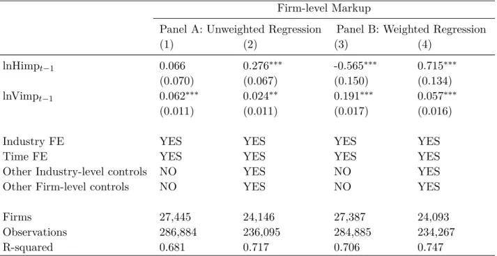
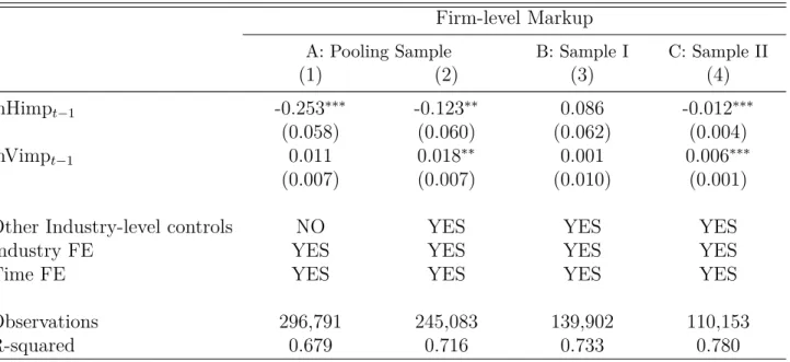
In column (3) and (4), we implement a weighted regression specification having as weight the number of observations in each 6-digit BEA Input-Output industry that are used in the esti-mation of production function in each 2-digit sector. And this magnitude stays stable for these weighted regressions in columns (3) and (4): the coefficient of vertical import penetration in-creases to 1.23 and remains unchanged when including controls.We test our primary hypothesis further using firm-level observations. In particular, we regress firm-level markups over 6-digit industrial import penetration rations as in Acemoglu et al. (2016) and Olper et al. (2017),15
lnµist=β1lnHIM Pst−1+β2lnV IM Pst−1+Zist0 γ+β4Ist+θi+σs+δt+εst (27)
wherelnµistis the markup of the firmi, who operates in industrysat yeartin equation 27. The
firm characteristic vectorFitis added to account for time-variant firm-level factors including the
number of employment, capital-labor ratio, and productivity that could also influence a firm’s capacity of adjusting markups. We also include firm fixed-effects as captured byθi.
Table 5 reports the results from the firm level regressions. We find a positive and strongly significant correlation between both types of penetration ratios and the value of markup. Ac-cording to the results from the unweighted regression specification estimation, implies that a 10% increase of vertical import penetration contributes to .62% and .25% increase of firm-level markup without and with other firm and industry controls. Columns (3) and (4) in Table 5 further reports the firm-level baseline results of weighted regression. Our results show a more significant positive correlation between the vertical import penetration ratio and the markup and they increase in scale comparing to unweighted regressions in column (1) and (2).
15In these regressions, we still use the industrial level data for the variables horizontal and vertical penetration
4.2
Mechanisms
Here we further verify the main results presented above by looking into the specific mechanisms that operate in our theoretical model.
4.2.1 Production Frontier
Our model predicts that firms are motivated to employ more foreign inputs when variable ing cost decreases, but only firms with relatively high initial productivity can pay the fixed sourc-ing costs, import foreign intermediate goods and obtain the correspondsourc-ing market advantage. Therefore, we should be able to observe that the positive effect of vertical import penetration is more substantial for firms that are initially at the fringe of the productivity frontier. We interact vertical import penetration ratio with a measure of the firm’s position relative to the produc-tion frontier. We define a firm’s proximity to the frontier as the ratio of its initial estimated productivityλiniit to the highest productivity of that year in the industry the firm belongs to as in Amiti and Khandelwal (2013): P Fit =
λini it
maxi∈s(λiniit )
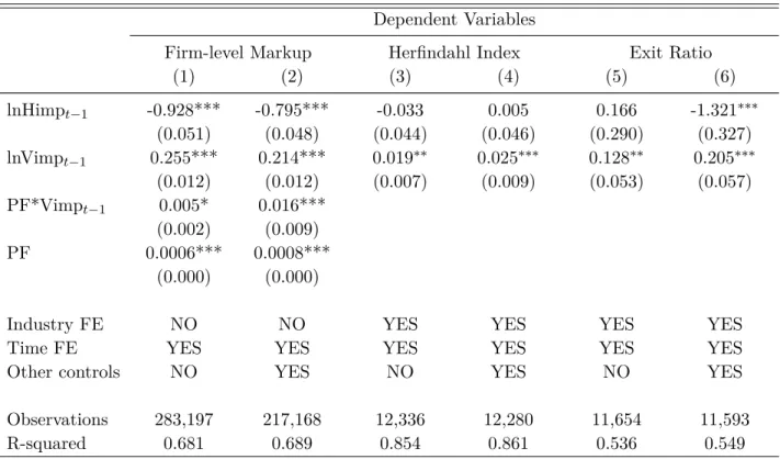
. Table 6 column (1) shows a significant positive effect of the vertical import penetration ratio to markup and the significant positive coefficient of the interaction term between vertical import penetration and production frontier measure indicates the impact is more profound for firms initially at the fringe of productivity frontier. This relationship remains stable with the addition of firm and industry level controls as shown in column (2).
4.2.2 Industry Concentration
To fully understand the impacts of vertical import penetration on domestic market structure, we use HHI index as a measure of market concentration and look at how vertical import penetration may contribute to the reshaping of market structure. Table 6 shows a positive effect of the vertical import penetration ratio but a negative effect of the horizontal import penetration
intensity on the market concentration. The reports from Table 6 column (3) and (4) indicate that when the high productivity firms use more ratio of foreign inputs, the low productivity firms will face higher competition pressure from the high productivity firms and the market exiting ratio rises as well.
4.2.3 Industry Exit ratio
The rest of Table 6 relates the percentage of firms’ exit in each industry with the import penetra-tion measures. The central predicpenetra-tion on the relapenetra-tionship between vertical import penetrapenetra-tion and markup relies on the differential impacts that import penetration has on heterogeneous firms. We thus expect to observe more firms exiting the market as high productivity firms re-tain cost advantage through importing intermediate inputs. The positive coefficients of vertical import penetration on industry exit ratio reported in Table 6 column (5) and (6) indicate that when the high productivity firms use more foreign inputs, the low productivity firms will face higher competition pressure from the high productivity firms and the market exiting ratio thus rises.
To sum up our results, we test the predicted mechanism of our model: the effect on markup is more profound for firms initially at the fringe of the productivity frontier. This is expected in the model as only firms with relatively high productivity could pay the fixed cost of sourcing intermediate goods from foreign countries and benefit more in the process of globalization. After this, we look at the change of both HHI and firms’ exit ratio of each industry concerning the shift of import penetration. They further validate our expectation: the industry’s sales are more concentrated to the advantageous firms, and the low productivity firms are forced to exit the market and so the firms’ exit ratio of the industry increases.