Robust 3D Scan Point Classification
using Associative Markov Networks
Rudolph Triebel and Kristian Kersting and Wolfram Burgard
Department of Computer Science, University of FreiburgGeorge-Koehler-Allee 79, 79108 Freiburg, Germany Email:{triebel, kersting, burgard}@informatik.uni-freiburg.de
Abstract— In this paper we present an efficient technique to learn Associative Markov Networks (AMNs) for the segmentation of 3D scan data. Our technique is an extension of the work
recently presented by Anguelov et al. [1], in which AMNs are
applied and the learning is done using max-margin optimization. In this paper we show that by adaptively reducing the training data, the training process can be performed much more efficiently while still achieving good classification results. The reduction is obtained by utilizing kd-trees and pruning them appropriately. Our algorithm does not require any additional parameters and yields an abstraction of the training data. In experiments with real data collected from a mobile outdoor robot we demonstrate that our approach yields accurate segmentations.
I. I
Recently, the problem of acquiring three-dimensional mod-els using mobile robots has become quite attractive and a variety of robot systems have been developed that are able to acquire three-dimensional data using laser range scanners [2]– [8]. Most of these approaches are focused on the problem of how to improve the localization of the robot or how to reduce the huge amount of data by piecewise linear approximations. In this paper we consider the problem of classifying data points in three-dimensional range scans into known classes. The general motivation behind this is to achieve the ability to learn maps that are annotated with symbolic labels. In the past, it has been shown that such information can be utilized to find compact representations of the maps [8], but also to improve the process of joining partial maps into one big map, usually called map registration [9], [10]. When using annotated maps, the registration can be performed by finding corresponding annotated objects in the partial maps, which is usually much more effective and reliable compared to finding correspondences on the raw data level.
The approach we present in this paper to find map anno-tations or labelsis formulated as a supervised learning task. Given a set of manually annotated data, our systemlearnsa set of parameters from this map, which are later used to classify a new and unlabeled map. Throughout this paper, this final step will be referred to as inference. The parameter learning step is essentially a maximum likelihood estimation process where the likelihood of the labels for the given data is maximized.
An important detail of each classification technique is the way the dependency between labels and data is modeled. For example, one can assume that the labels only depend on the local evidence of each data point. This is equivalent to
assuming statistical independence of neighboring data points and can be found in many applications. However, recent results show that a higher classification accuracy can be achieved when considering the problem as a global classification task, i.e., when we view the data not independently, because the labeling of a data point is also influenced by the labeling of other data points in the vicinity of the point in question. This approach is known ascollective classification[11].
One popular approach for the task of collective classification are Relational Markov Networks (RMNs) [12]. In addition to the labels of neighboring points, RMNs also consider the relations between different object classes. E.g., we can model the fact that two classes AandBare more strongly related to each other than, say, classesA andC. This modeling is done on the abstract class level by introducingclique templates[12]. Applying these clique templates to a given data set yields an ordinary Markov Network (MN). In this unrolled MN, the result is a higher weighting of neighboring points with labels
A andB than of points labeled AandC. One type of RMNs for which efficient algorithms for learning and inference are available, areAssociative Markov Networks(AMNs).
RMNs, and in turn AMNs, can be viewed as a method of viewing the data at a higher level of abstraction. This abstraction is done in the description of the model and not in the unrolled MN. Thus, abstraction has been considered only in the feature space. The main contribution of this paper is to investigate methods of additional abstraction in AMNs by utilizing the geometry of the data. As our experiments demonstrate, this accelerates the training process and does not decrease the classification performance.
This paper is organized as follows. After discussing re-lated work in the following section we define our scan-point classification approach in Section III. Then, we introduce Markov Random Fields and discuss how they can be used to utilize the classification of neighboring points to improve the segmentation. Section V describes the variants of the learning and inference algorithms used in our current system. Section VI is concerned with our compact representation of the data points. Finally, Section VII presents experimental results illustrating the usefulness of our approach.
II. RW
In the area of mobile robotics many authors have consid-ered the problem of extracting features from range data. For
example, Buschka and Saffiotti [13] describe a virtual sensor that is able to identify rooms from range data. Additionally, Simmons and Koenig, [14] use a pre-programmed routine to detect doorways from range data. Althaus and Christensen [15] use line features to detect corridors and doorways. Also several authors focused on the problem of extracting planar structures from range scans. For example, H¨ahnel et al. [16] use a region growing technique to identify planes. Recently, Liu et al. [3], Martin and Thrun [17], as well as Triebel et al. [8] applied variants of the expectation maximization algorithm (EM) to cluster range scans into planes. Furthermore, there has been work on employing features extracted from three-dimensional range scans to improve the scan alignment pro-cess [9], [10]. The approaches described above either operate on two-dimensional scans, consider single features such as planarity, or apply pre-programmed routines to identify the features in range scans. In a recent work, M´artinez-Mozoset al.[18] presented an approach that uses features extracted from a two-dimensional laser range scans and applies the Adaboost algorithm to identify what type of place the robot is at. This approach, however, classifies the entire scan and does not label individual points in range scans.
In the context of learning annotated 3D maps from point cloud data, the approaches that have been presented previously differ in the selection of the features to be extracted and in the learning strategies. For example, spin images have been introduced as a type of rotation invariant features by Johnson and Hebert [19]. Ruiz-Correa et al. apply spin images to recognize deformable shapes [20]. Frome et al. extend spin images to point descriptors and apply a voting technique to recognize objects in range data [21]. Vandapel et al. [22] extract saliency features based on the eigenvalues of local covariance matrices and apply EM to learn a Gaussian Mixture Model classifier. Another object description technique is called
shape distributionsand has been applied by Osadaet al.[23]. In contrast to these approaches, our algorithm classifies the data by incorporating knowledge of neighboring data points. This is modeled in a mathematical framework known as Markov random fields and improves the segmentation by elim-inating false classifications. Our approach is an improvement over the work proposed by Anguelov et al. [1] in the sense that it adaptively selects data points from the training data set and uses these points as representatives for neighboring points. This way, the training data set is reduced in size to an abstraction of the original range scan. As a result, our approach requires less complex constraints and, in turn, yields a faster training phase without decreasing classification rates.
III. SPC
Suppose we are given a set of N scan points p1, . . . ,pN
taken from a 3D scene and a set of K object classes C1, . . . ,CK. The task is now to find alabel yi∈ {1, . . . ,K}for
each scan pointpiso that all labelsyi, . . . ,yNare optimal given
the scan points. By “optimal” we mean that the likelihood of the labels given the data is maximized. We will see later how this likelihood is defined. In this paper, the classification
task will be formulated as a supervised learning problem. This means, there is a set of scan points to which the correct labels have been assigned by hand, the training set, and a set of unlabeled points, the test set. The classification process is divided into two phases: the learning phase and the inference phase.
A. Feature Extraction
When labeling 3D range data we want to add semantic information which is independent of the geometry of the input data. For example, in a setting, where we want to distinguish window frames from the wall of a building, the window points may occur in any 3D position. Thus, to be able to divide the scan points into different classes, we need to extract features from the input data. We will represent these features as a vector
xiof non-zero values for each scan pointpi. The vector of all
feature vectorsxiwill be denoted asx. Using this notation, we
can formulate the inference problem as finding the set of labels
y that maximizes the conditional probabilityPω(y|x), where
ω is a set of parameters defining the underlying probability density function. If we defineˆyas the vector of correct labels ˆ
y1, . . . ,yˆN, the learning task can be formulated as finding the
parameters ω that maximize the probability Pω(ˆy | x). In summary, learning and inference can be written as:
learning: ω∗=argmaxωPω(ˆy|x) (1) inference: y∗ =argmaxyPω∗(y|x) (2)
IV. MRF
One possible way to define Pω is to assume a normal distribution of the features in each class. In this case, ω
consists of the means µk and covariance matrices σk
corre-sponding to each class. Then, the probability Pω(y | x) is represented as a multi-modal normal distribution where each mode corresponds to one object class. The learning task is performed by determining (µk, σk) for k = 1, . . . ,K and the
inference is done by assigning the class label Ck to each xi
for which the corresponding normal distributionN(xi;µk, σk)
is maximal. This method is called Bayes classification [24] and is applied in various classification tasks.
One problem with the Bayes classifier is that often the labeling of a data point does not only depend on its local features, but also on the labeling of nearby data points. For example, if we consider the local planarity of a scan point as a feature, it may happen that the class label ‘wall’ is more likely than the class label ‘door’, although all other scan points in the vicinity of this point belong to the class ‘door’. Methods that use the information of neighboring data points are called
collective classification [11]. A popular framework in this context areMarkov Random Fields (MRFs).
A. Description
A Markov Random Field is an undirected graph with a set of cliques C and a clique potential φc, which is a
classification, we considerconditionalMRFs [12] defining the distribution P(y|x)= Q c∈Cφc(xc,yc) P y′Qc∈Cφc(xc,y′c) (3) where xc and yc are the features and labels of all nodes in
the cliquec. Here, the potentialφcis a mapping from features
and labels to a positive value. This value is often called the
compatibility between the features and the labels of the data points inc. The higher the compatibility is, the more likely it is that the labels yc are correct for the featuresxc.
The denominator in equation (3) is called the partition function, usually denotedZ, and is essentially a sum over all possible labelings. In all but the simplest cases the calculation of the partition function constitutes the major problem in the learning task because of its exponential complexity. We will later see how learning can be done without calculating Z.
B. Associative Markov Networks
To simplify the problem, the size of the cliques is usually restricted to be either one or two. This results in a pairwise
MRF, where only node and edge potentials ϕ and ψ are considered. For a pairwise MRF with the set of edges E = {(i j)|i< j} equation (3) simplifies to P(y|x)= 1 Z N Y i=1 ϕ(xi,yi) Y (i j)∈E ψ(xi j,yi,yj). (4)
Again, Z denotes the partition function given by Z =
P
y′QiN=1ϕ(xi,y′
i)
Q
(i j)∈Eψ(xi,y′i,y′j). Note that in equation (4)
there is a distinction between node featuresxi∈dn and edge
featuresxi j ∈de. Thus, the numberdn of node features and
the numberde of edge features is not necessarily the same.
It remains to describe the potentialsϕandψ. As mentioned above, the potentials reflect how well the features fit to the labels. One simple way to define the potentials is thelog-linear
model [25]. In this model, a weight vector wk is introduced
for each class labelk=1, . . . ,K. The node potentialϕis then defined so that logϕ(xi,yi)=wkn·xiwherek=yi. Accordingly,
the edge potentials are defined as logψ(xi j,yi,yj) = wke,l·xi
where k=yi and l=yj. Note that there are different weight
vectors wk
n ∈dn andw k,l
e ∈de for the nodes and edges.
For the purpose of convenience we use a slightly different notation for the potentials, namely
logϕ(xi,yi) = K X k=1 (wkn·xi)yki (5) logψ(xi j,yi,yj) = K X k=1 (wke,l·xi j)ykiy l j, (6) where yk
i is an indicator variable which is 1 if point pi has
label kand 0, otherwise.
In a further refinement step of our model, we introduce the constraints wke,l = 0 for k , l and wke,k ≥ 0. This results in
ψ(xi j,k,l)=1 for k,l andψ(xi j,k,k) =λki j, where λki j ≥1.
The idea here is that edges between nodes with different labels
should be penalized over edges between equally labeled nodes. A pairwise MRF with these restrictions is called anAssociative Markov Network(AMN).
V. L I AMN
In this section, we describe how learning and inference can be done with AMNs according to equations (1) and (2). In a first step, we reformulate the problem so that, instead of maximizing Pω(y | x), we maximize logPω(y | x). The parameters ω are represented by the weight vectors w =
(wn,we). By plugging in equations (5) and (6), we obtain
max N X i=1 K X k=1 (wkn·xi)yki + X (i j)∈E K X k=1 (wke·xi j)ykiy k j−logZw(x). (7) Note that the partition function Z only depends onw andx, but not on the labelsy.
A. Learning
The problem arising in the learning task is that the partition functionZ depends on the weights w. This means that when maximizing logPw(ˆy|x) the intractable calculation ofZneeds to be done for each w. However, if we instead maximize the
marginbetween the optimal labeling ˆyand any other labeling
y defined by
logPω(ˆy|x)−logPω(y|x), (8) the termZw(x) cancels out and the maximization can be done efficiently. This method is referred to as maximum margin
optimization. The details of this formulation are omitted here for the sake of brevity. We only note that the problem is reduced to a quadratic program (QP) of the form:
min 1 2kwk 2+cξ (9) s.t. wXˆy+ξ− N X i=1 αi≥N; we≥0; αi− X i j,ji∈E αki j−wk n·xi≥ −yˆki, ∀i,k; αki j+αkji−wek·xi j≥0, αki j, α k ji≥0, ∀i j∈E,k
Here, the variables that are solved for in the QP are the weights
w =(wn,we), a slack variable ξ and additional variables αi,
αi j andαji. Again, we refer to Taskaret al. [25] for details. B. Inference
Once the optimal weights w are calculated, we can do inference on an unlabeled test data set. This is done by finding the labelsythat maximize logPw(y|x). As mentioned above, Z does not depend on y so that the maximization in equation (7) can be done without considering the last term. With the constraints imposed on the variablesyk
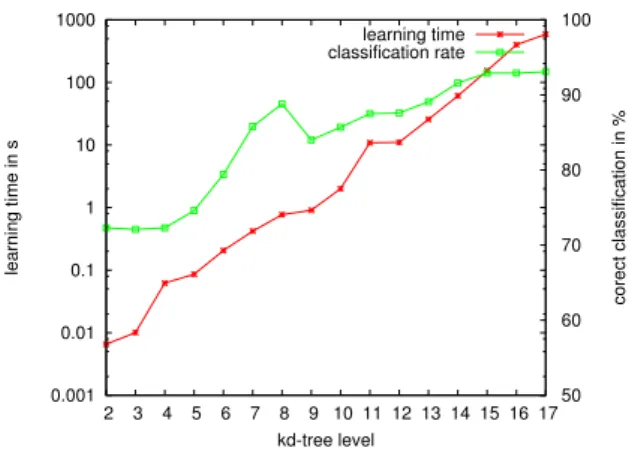
0.001 0.01 0.1 1 10 100 1000 2 3 4 5 6 7 8 9 10 11 12 13 14 15 16 17 50 60 70 80 90 100 learning time in s corect classification in % kd-tree level learning time classification rate
Fig. 1. Processing time for the learning task (red with crosses) and
classification rate (green with boxes) for different values ofdmax. The left
y-axis is for the time and is shown in log-scale, the right one is for the classification results.
a linear program of the form max N X i=1 K X k=1 (wkn·xi)yki + X i j∈E K X k=1 (wke·xi j)yki j (10) s.t. yki ≥0, ∀i,k; K X k=1 yi=1, ∀i yki j≤yki, yi jk ≤ykj, ∀i j∈E,k
Here, we introduced variables yk
i j representing the labels of
two points connected by an edge. The last two inequality conditions are a linearization of the constraint yk
i j =y k i ∧y k j. VI. DR
Unfortunately, the learning task we described in the previous section is computationally expensive in run time as well as in memory requirement. For each scan point there is one variable and one constraint in the quadratic program (9). Furthermore, we have two variables and two constraints per edge. This results in a large computational effort; Anguelov
et al. [1] report one hour run time for about 30,000 scan points. Fortunately, in usual data sets, a huge part of the data is redundant. For instance, to reduce the data set we can randomly draw a smaller set of scan points from the whole scan. In our experiments this gives good results. The run time dropped down from about 20 minutes down to less than a minute while the detection rate was still around 92%. However, it is not clear how many samples are necessary to obtain good detection rates, because this depends on the data set. A scene with many small objects should not be down-sampled as much as a scene with only few, big objects. Therefore we reduce the data adaptively.
A. Adaptive Reduction
The idea of adaptive data reduction is to obtain as much information as necessary from the training data so that still a good recognition rate can be achieved. This is dependent on the data set, so we need an adaptive data structure. One popular
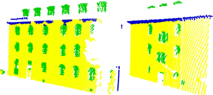
Fig. 2. The resulting AMN after reducing the training data (see fig. 3(a)). By applying the adaptive reduction, the borders between labeled regions are emphasized while areas in which the labels do not change are represented in a higher level of abstraction.
way to adaptively store geometrical data are kd-trees [10]. The way the data is stored in kd-trees is that of a coarse-to-fine structure: on higher levels of the tree the level of data abstraction is also higher. By utilizingkd-trees we can reduce the data set by considering only scan points in the tree that are stored in leaf nodes up to a given maximum depth dmax.
All points in deeper branches are then merged into a new leaf node of depth dmax. The data point in this new leaf node is
calculated as the mean of all points from the corresponding subtree. Apart from the reduction in the data complexity, this has the advantage of a sampling that is less dependent on the data density. The only question here is how to selectdmax.
To investigate the influence of the maximal tree depth we ran the recognition process with different values for dmax.
Figure 1 shows the time the training process took and the corresponding classification rate for each value ofdmax. What
can be seen from the figure is that the processing time grows exponentially whereas the recognition rate does not improve for dmax higher than 15. For dmax = 15 we obtained a
classification rate of 92.9% while the run time for the training was only 2.5 minutes. In this case, the training set consisted of 6558 points.
B. Parameterless Reduction
When using kd-trees to reduce the training data in the described way, it still remains to find a good value fordmax. As
for the uniform down-sampling, this is dependent on the data set. In our current system, we therefore modify the reduction algorithm so that it is parameter-free: We still use akd-tree to store the data points, but instead of pruning at a fixed level, we merge all points in a subtree whenever all of its labels are equal. The idea here is that for large homogeneous areas, where all points have the same label, we can assume a higher level of abstraction as in heterogeneous areas.
Figure 2 shows an example of a training set that was reduced in this way. The original data set is shown in figure 3(a). The reduced set consists only of 919 points, while the original scan contained 16,917 labeled points. As the next section will show,
Fig. 4. Additional results on two other data sets for the AMN learner with adaptive data reduction.
training on a data set, which was reduced this way, took only a few seconds. This is a substantial speed-up without a serious reduction of the classification performance.
VII. ER
We applied the described classification algorithm to real data collected with a SICK laser range finder mounted on top of a pan/tilt unit. The data consisted of 3D outdoor scans from a building with different kinds of windows. In a first step, we divided the data into walls by using a plane extraction algorithm. For each wall we obtained a normal vectornand a mean pointq. Then we extracted all points that had a distance of at most 0.5m from the planes. In this way we achieve robustness against noise from the normal vector calculation.
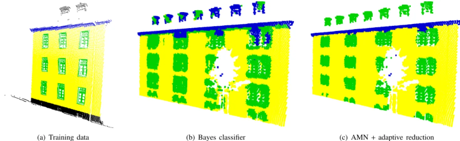
The goal was to classify the scan points into the classes ‘window’, ‘wall’ and ‘gutter’. One of the data sets together with its manually created labeling is shown in figure 3(a). It represents one wall of the building with only single-size windows. For the evaluation we used three different scans of walls of the building with single- and double-size windows.
A. Feature Extraction
We evaluated different types of features. It turned out that good results can be achieved with feature vectors that represent a local distribution of some value. One such distribution we used in the experiments was that of the cosine of the angles between the local normal vectors in the vicinity of each point and the plane normal vector n. For a neighbor p′
i of
a given scan point this value is calculated by α:=p′
i·n. The
distribution over αis represented as a local histogram. Another set of features was obtained by considering the distribution of neighbors in front of and behind the wall plane. To be more precise, at each scan point pi we counted the
number of neighbors p′
i so that |p ′
i ·n|> |p·n|+ǫ whereǫ
was used as a threshold to get robustness against noise. In our experiments,ǫwas set to 0.05m. Accordingly, we counted the neighbors so that |p′
i·n|<|p·n| −ǫ and|p·n| −ǫ≤ |p ′ i·n| ≤ |p·n|+ǫ. This way we obtained a histogram with three bins. The last feature we used was the normalized height of each scan point. Here, we assumed a maximum scan height hmax
of 15mwhich is reasonable considering that objects that are higher than 15mcannot be scanned accurately. For points with negative height, this feature was set to 0. For all others it was
the quotient of the local height and hmax. This feature was
especially used to distinguish ‘gutter’ from the other classes.
B. Building the Markov Network
An important implementation detail is the way the nodes are connected in the network. If we take too many neighbors, the learning and the inference will be less efficient and require a lot of time. Also, the way in which the connections are defined has an influence on the classification result. For our experiments, it turned out that a sampling strategy similar to the one Anguelov et al. [1] report gives the best results. In our case, we randomly sample neighbors for each scan point
pi using a Gaussian distribution. Then we connect pi to its
neighbors so that no point is connected to more than three others. This guarantees that learning and inference can be carried out efficiently and at the same time provides enough information from the neighboring points.
C. Evaluation
The experimental results are shown in Figures 3 and 4. For comparison, we ran a Bayes classification on the same data set, yet with a different set of features. The reason for this is that in Bayes classification the features are assumed to be distributed normally and this did not hold in the case of our features. The best result we obtained is shown in figure 3(b). It can be seen that in some regions the classes are locally inconsistent. Especially in the roof windows, the classification is wrong. This is because the Bayes classifier only decides locally on the labels and does not take the neighbors into account.
Figure 3(c), shows the result for the same data set obtained with the AMN approach. Additionally, figure 4 shows the results for two other test instances. For solving the QP in the learning step we used the C++library OOQP [26].
For quantitative evaluation we labeled one of the test sets by hand and compared the results with this labeling. We obtained 85.5% correct classifications for the Bayes classifier and 93.8% for the AMN with adaptive data reduction. The computation time for the learning step was between 5 and 7 seconds on a Pentium 4 with 2.8 GHz.
VIII. C FW
In this paper we presented an approach to segment three-dimensional range data. Our approach uses Associative Markov Networks to robustly extract these regions based on an initial labeling obtained with simple geometric features. To efficiently carry out the learning phase, we use an adaptive technique to prune the the kd-tree. This allows us to efficiently deal with even large data sets. Thereby, the robustness of the segmentation process is maintained.
Our approach has been implemented and tested on data acquired with an outdoor-robot equipped with a laser range finder mounted on a pan/tilt unit. In complex data sets con-taining outer walls of buildings, our approach has successfully been applied to the task of finding a segmentation into walls, windows, and gutters. In a comparison experiment we could
(a) Training data (b) Bayes classifier (c) AMN+adaptive reduction
Fig. 3. (a): Data set used for training. The black points are unlabeled and are not considered in the training process. (b): Classification result using Bayes classification. Especially at the borders between classes the classification is poor. (c): Result using AMN and adaptive data reduction.
furthermore demonstrate that our approach yields more robust classifications than the Bayes classifier.
The data reduction technique presented here is motivated by the idea of finding geometrical abstractions for the training data. This assumes that by the abstraction no information about the mapping between features and labels is lost in the learning step. In our experiments this was never the case. However, there can be cases where this assumption is violated, especially when the features of points inside a class are distributed very sparsely. This problem is subject to ongoing investigations.
A
This work has partially been supported by the German Research Foundation under contract number SFB/TR8, by the European Commission under contract number FP6-508861, and by the German Federal Ministry of Education and Re-search (BMBF) under contract number 01IMEO1F.
R
[1] D. Anguelov, B. Taskar, V. Chatalbashev, D. Koller, D. Gupta, G. Heitz, and A. Ng, “Discriminative Learning of Markov Random Fields for
Segmentation of 3D Range Data,” inConference on Computer Vision
and Pattern Recognition (CVPR), 2005.
[2] S. Thrun, W. Burgard, and D. Fox, “A real-time algorithm for mobile robot mapping with applications to multi-robot and 3D mapping,” in Proc. of the IEEE International Conference on Robotics&Automation (ICRA), 2000.
[3] Y. Liu, R. Emery, D. Chakrabarti, W. Burgard, and S. Thrun, “Using
EM to learn 3D models with mobile robots,” in Proceedings of the
International Conference on Machine Learning (ICML), 2001. [4] A. N ¨uchter, H. Surmann, and J. Hertzberg, “Planning robot motion for 3d
digitalization of indoor environments,” inProc. of the 11th International Conference on Advanced Robotics (ICAR), 2003.
[5] C. Fr¨uh and A. Zakhor, “3D model generation for cities using aerial photographs and ground level laser scans,” inProc. of the IEEE Com-puter Society Conference on ComCom-puter Vision and Pattern Recognition (CVPR), 2001.
[6] O. Wulf, K. Arras, H. Christensen, and B. Wagner, “2d mapping of cluttered indoor environments by means of 3d perception,” inProc. of the IEEE International Conference on Robotics&Automation (ICRA). [7] A. Georgiev and P. Allen, “Localization methods for a mobile robot in
urban environments,” vol. 20, no. 5, pp. 851–864, 2004.
[8] R. Triebel and W. Burgard, “Using hierarchical EM to extract planes from 3d range scans,” inProc. of the IEEE International Conference on Robotics&Automation (ICRA), 2005.
[9] ——, “Improving simultaneous localization and mapping in 3d using global constraints,” inProc. of the Twentieth National Conference on Artificial Intelligence (AAAI), 2005.
[10] A. N ¨uchter, O. Wulf, K. Lingemann, J. Hertzberg, B. Wagner, and
H. Surmann, “3d mapping with semantic knowledge,” in RoboCup
International Symposium, 2005.
[11] S. Chakrabarti and P. Indyk, “Enhanced hypertext categorization using hyperlinks,” inProc. of the ACM SIGMOD, Seattle, Washington, 1998. [12] B. Taskar, P. Abbeel, and D. Koller, “Discriminative probabilistic models for relational data,” inEighteenth Conference on Uncertainty in Artificial Intelligence (UAI02), Edmonton, Canada, August 2002.
[13] P. Buschka and A. Saffiotti, “A virtual sensor for room detection,” in Proc. of Intern. Conf. on Intelligent Robots and Systems (IROS), 2002. [14] S. Koenig and R. Simmons, “Xavier: A robot navigation architecture based on partially observable markov decision process models,” in Artificial Intelligence and Mobile Robots, D. Kortenkamp, R. Bonasso,
and R. Murphy, Eds. MIT Press, 1998.
[15] P. Althaus and H. Christensen, “Behaviour coordination in structured environments,”Advanced Robotics, vol. 17, no. 7, pp. 657–674, 2003. [16] D. H¨ahnel, W. Burgard, and S. Thrun, “Learning compact 3d models
of indoor and outdoor environments with a mobile robot,”Robotics and Autonomous Systems, vol. 44, pp. 15–27, 2003.
[17] C. Martin and S. Thrun, “Online acquisition of compact volumetric maps with mobile robots,” inIEEE International Conference on Robotics and Automation (ICRA). Washington, DC: ICRA, 2002.
[18] O. M. Mozos, C. Stachniss, and W. Burgard, “Supervised learning of places from range data using adaboost,” inProc. of Intern. Conference on Robotics and Automation (ICRA), 2005.
[19] A. Johnson and M. Hebert, “Using spin images for efficient object recognition in cluttered 3d scenes,” IEEE Transactions on Pattern Analysis and Machine Intelligence, vol. 21, no. 5, pp. 433–449, 1999. [20] S. Ruiz-Correa, L. G. Shapiro, M. Meila, and G. Berson,
“Discrimi-nating deformable shape classes,” inAdvances in Neural Information Processing Systems (NIPS), 2004.
[21] A. Frome, D. Huber, R. Kolluri, T. Bulow, and J. Malik, “Recognizing objects in range data using regional point descriptors,” inProceedings of the European Conference on Computer Vision (ECCV), 2004. [22] N. Vandapel, D. Huber, A. Kapuria, and M. Hebert, “Natural terrain
classification using 3-d ladar data,” in IEEE International Conference on Robotics and Automation, 2004.
[23] R. Osada, T. Funkhouser, B. Chazelle, and D. Dobkin, “Matching 3d models with shape distributions,” inShape Modeling International, Genova, Italy, 2001.
[24] S. Theodoridis and K. Koutroumbas, Pattern Recognition. Elsevier Academic Press.
[25] B. Taskar, V. Chatalbashev, and D. Koller, “Learning Associative Markov Networks,” inTwenty First International Conference on Machine Learn-ing, 2004.
[26] E. M. Gertz and S. J. Wright, “Object-oriented software for quadratic programming,” ACM Transactions on Mathematical Software, no. 29, pp. 58–81, 2003.