Improving HPC Application Performance in Cloud
through Dynamic Load Balancing
Abhishek Gupta, Osman Sarood, Laxmikant V Kale University of Illinois at Urbana-Champaign
Urbana, IL 61801, USA (gupta59, sarood1, kale)@illinois.edu
Dejan Milojicic HP Labs Palo Alto, CA, USA [email protected]
Abstract—Driven by the benefits of elasticity and pay-as-you-go model, cloud computing is emerging as an attractive alternative and addition to in-house clusters and supercomputers for some High Performance Computing (HPC) applications. However, poor interconnect performance, heterogeneous and dynamic environ-ment, and interference by other virtual machines (VMs) are some bottlenecks for efficient HPC in cloud. For tightly-coupled iterative applications, one slow processor slows down the entire application, resulting in poor CPU utilization.
In this paper, we present a dynamic load balancer for tightly-coupled iterative HPC applications in cloud. It infers the static hardware heterogeneity in virtualized environments, and also adapts to the dynamic heterogeneity caused by the interference arising due to multi-tenancy. Through continuous live monitor-ing, instrumentation, and periodic refinement of task distribution to VMs, our load balancer adapts to the dynamic variations in cloud resources. Through experimental evaluation on a private cloud with 64 VMs using benchmarks and a real science appli-cation, we demonstrate performance benefits up to 45%. Finally, we analyze the effect of load balancing frequency, problem size, and computational granularity (problem decomposition) on the performance and scalability of our techniques.
Keywords-High Performance Computing; Cloud; load-balance;
I. INTRODUCTION
The ability to rent (using pay-as-you-go model) rather than own a cluster makes cloud a cost-effective and timely solution for the needs of some academic and commercial HPC users, especially those with sporadic or elastic demands. In addition, virtualization support in cloud allows better flexibility and cus-tomization to specific application, software, and programming environment needs of HPC users. Cloud providers, such as Amazon EC2 [1], make profit due to economies of scale and high resource utilization enabled by multi-tenancy, virtualiza-tion, and overprovisioning of typical web-service loads.
However, despite these benefits, prior research has shown that there is a mismatch between characteristics of cloud en-vironment and HPC requirements [2–5]. HPC applications are typically tightly-coupled, and perform frequent inter-processor communication and synchronization. The insufficient network performance is a major bottleneck for HPC in cloud, and has been widely explored [2–5]. Two less explored challenges are resource heterogeneity and multi-tenancy – which are fundamental artifacts of running in cloud. Clouds evolve over time, leading to heterogeneous configurations in processors, memory, and network. Similarly, multi-tenancy is also intrinsic
of cloud, enhancing the business value of providing a cloud. Multi-tenancy leads to multiple sources of interference due to sharing of CPU, cache, memory access, and interconnect. For tightly-coupled HPC applications, heterogeneity and multi-tenancy can result in severe performance degradation and un-predictable performance, since one slow processor slows down the entire application. As an example, on 100 processors, if one processor is30% slower compared to the rest, application will slowdown by30% even though the system has99.7% raw CPU power compared to the case when all processors are fast. One approach to address the above problem is mak-ing clouds HPC-aware; examples are HPC-optimized clouds (such as Amazon Cluster Compute [6] and DoE Magellan project [4]) and HPC-aware cloud schedulers [7, 8]. In this work, we explore the other approach – making HPC cloud-aware, which is relatively less explored [9, 10].
Building on our previous work [10], our primary hypothesis is that the challenges of heterogeneity and noise arising from multi-tenancy can be handled by an adaptive parallel runtime system. To validate our hypothesis, we explore the adaptation of Charm++ [11, 12] runtime system to virtualized environment. We present techniques for virtualization-aware load balancing to help application users gain confidence in the capabilities of cloud for HPC. MPI [13] applications can also benefits from our approach using Adaptive MPI (AMPI) [12]. Also, our fundamental approach is applicable to other pro-gramming models which support migratable work/data units.
Efficient load balancing in a cloud is challenging since run-ning in VMs makes it difficult to determine if (and how much of) the load imbalance is application-intrinsic or caused by extraneous factors. Extraneous factors include heterogeneous resources, other users’ VMs competing for shared resources, and interference by virtualization emulator process (§II).
The primary contributions of this work are the following: • We propose dynamic load balancing for efficient
exe-cution of tightly-coupled iterative HPC applications in heterogeneous and dynamic cloud environment. The main idea is periodic refinement of task distribution using measured CPU loads, task loads, and idle times (§IV). • We implement these techniques in Charm++ and evaluate
their performance and scalability on a real cloud setup on Open Cirrus testbed [14]. We achieve 45% reduction in execution time compared to no load balancing (§VI).
• We analyze the impact of load balancing frequency, grain size, and problem size on achieved performance (§VI). II. NEED FORLOADBALANCER FORHPCINCLOUD In the context of cloud, the execution environment depends on VM to physical machine mapping, which makes it (a) dynamic and (b) inconsistent across multiple runs. Hence, a static allocation of compute tasks to parallel processes would be inefficient. Most existing dynamic load balancing techniques operate based exclusively on the imbalance internal to the application, whereas in cloud, the imbalance might be due to the effect of extraneous factors. These factor originate from two characteristics, which are intrinsic to cloud:
1) Heterogeneity: Cloud economics is based on the cre-ation of a cluster from existing pool of resources and incremental addition of new resources. While doing this, homogeneity is lost.
2) Multi-tenancy: Cloud providers run a profitable business by improving utilization of underutilized resources. This is achieved at cluster-level by serving large number of users, and at server-level by consolidating VMs of complementary nature (such as memory- and compute-intensive) on same server. Hence, multi-tenancy can be at resource-level (memory, CPU), node-level, rack-level, zone-level, or data center level.
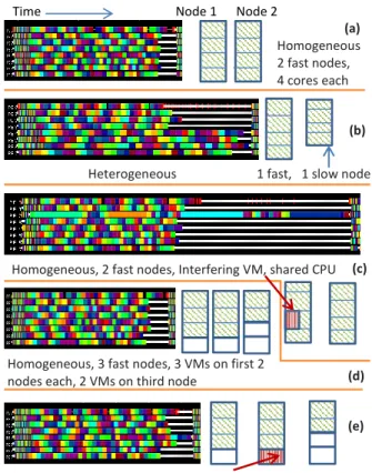
In such environment, application performance can severely degrade, especially for tightly-coupled applications where the application progress is governed by the slowest processor. To demonstrate its severity, we conducted a simple experiment where we ran a tightly-coupled 5-point stencil benchmark, referred to as Stencil2D (2K× 2K matrix), on 8-VMs, each with a single virtual core (VCPU), pinned to a different physical core of 4-core nodes. More details of our exper-imental setup and benchmarks are given in Section V. To study the impact of heterogeneity, we ran this benchmark in 2 cases - first, we used two physical nodes of same fast (3.00 GHz) processor type (Figure 1a) and second, we used two physical nodes with different processor types – fast (3.00 GHz) and slow (2.13 GHz) (Figure 1b). We used Projections [15] performance analysis tool. Figure 1 shows one iteration of these runs. Each horizontal line represents the timeline for a VM (or VCPU). Different colors (shades) represent time spent executing application tasks whereas white represents idle time. The length of timelines represent the iteration execution time, after which the next iteration can begin. In Figure 1a, the small idle time on VM#1-7 is present because the first process performs a small co-ordination work. In Figure 1b, there is lot more idle time (hence wastage of CPU cycles) on first four VMs compared to the next four, since VMs#4-7 running on slower processors take longer to finish same amount of work. Similar effect is also observed when there is an interfering VM. Figure 1c shows the case when we ran all VMs on fast processors but there is an interfering VM which shares the physical core with one of the VMs from our parallel job (VM#3). The interfering VM runs sequential NPB-FT (NAS Parallel Benchmark – Fourier Transform) Class A [16]. In this
(a) Homogeneous 2 fast nodes, 4 cores each
Time Node 1 Node 2
Heterogeneous 1 fast, 1 slow node
Homogeneous, 2 fast nodes, Interfering VM, shared CPU
Homogeneous, 3 fast nodes, 3 VMs on first 2 nodes each, 2 VMs on third node
(b)
(c)
(e)
Homogeneous, 3 fast nodes as in (d), interfering VM, shared node (d)
Fig. 1: Experimental setup (on right) and timeline of 8 VMs showing one iteration of Stencil2D: white portion = idle time, colored portions = application functions.
case, the Projections timelines tool includes the time spent executing the interfering task in the time spent for executing tasks of the parallel job on that processor because it can not identify when the operating system switches context. This gets reflected in the fact that some of the tasks hosted on VM#3 take significantly longer time to execute than others (longer bars in Figure 1c). Due to this CPU sharing, it takes longer for the parallel job to finish the same tasks. Moreover, the tightly-coupled nature of the application means that no other process can start the next iteration unless all processes have finished the current iteration (idle times on rest of the VMs). If the VMs do not share physical core but share the multi-core physical node, the contention for limited shared cache capacity and memory controller subsystem can manifest itself as another source of interference (Figure 1e). Here. we ran the 8 VMs on 3 fast nodes, with first three VMs on one node, next three VMs on second node, and last two VMs on third node. On second node, we placed another VM mapped to the unused core and ran NPB-LU Class B benchmark on it. The unused cores on first and third nodes are left idle. Figure 1e shows that VM#5 is taking longer time than the rest compared to the case with exactly same configuration but no interfering VM (Figure 1d). It can also be noted that the time in Figure 1d is slightly better than Figure 1a. This can be attributed to the fact that the shared resources in the 4-core node are shared between 4 processes in Figure 1a, but by only 3 in Figure 1d. The distribution of such interference is fairly random and unpredictable in a cloud. Hence, we need a mechanism to adapt to the dynamic variation in the execution environment.
III. BACKGROUND: CHARM++ANDLOADBALANCING Charm++ [11,12] is a message-driven object-oriented paral-lel programming system, which is used by large-scale scientific applications such as NAMD [17]. In Charm++, the program-mer needs to decompose (or overdecompose) the application into large number of medium grained pieces, referred to as Charm++ objects orchares. By overdecomposition, we mean that the number of objects or work/data units is greater than the number of processors. Each object consists of a state and a set of functions, including local and entry methods, which execute only when invoked from a local or remote processor through messages. The runtime system maps these objects onto available processors and they can be migrated across pro-cessors during execution. This message-driven execution and overdecomposition results in automatic overlap of computation and communication, and helps in hiding the network latency. MPI [13] applications can leverage the capabilities of Charm++ runtime using the adaptive implementation of MPI (AMPI [12]), where MPI processes are implemented as user-level threads by the runtime.
The overdecomposition of application into migratable ob-jects (or threads) facilitates dynamic load balancing, a concept central to our work. The runtime system instruments the application execution, and measures various statistics, such as computation time spent in each object, process time, and idle time. Using this measured data, the load balancer periodically re-maps objects to processors using a load balancing strategy. There is an inherent assumption that future loads will be almost same as the measured loads (principle of persistence) – which is true for most iterative applications.
IV. CLOUD-AWARELOADBALANCER FORHPC
In a cloud, the application user has access only to virtualized environment which hides the underlying platform heterogene-ity. Hence, for heterogeneity-awareness, we estimate the CPU capabilities for each VCPU, and use those estimates to drive the load balancing. An accurate performance prediction will depend on the application characteristics, such as FLOPS, number of memory accesses, and I/O demands. In this paper, we demonstrate the merits of heterogeneity-awareness using a simple estimation strategy, which works well in conjunc-tion with periodic refinement of load distribuconjunc-tion. We use a simple compute-intensive loop (Figure 2) to measure relative CPU frequencies, which are then used by the load balancing framework. Also, we assume that VMs do not migrate during runtime, and VCPUs are pinned to physical CPUs. We believe that these assumptions are valid for HPC in cloud since live migration leads to further noise and migration costs, and pin-ning VCPUs to physical CPUs results in better performance.
Other then the static heterogeneity, we need to address inter-fering tasks of other VMs, which can start and finish randomly. Hence, we propose a dynamic load balancing scheme which continuously monitors the loads for each VCPU and reacts to any imbalance. Our scheme uses task migration which enables the runtime to keep equal loads on all VCPUs. It is based on instrumenting the time spent on each task, and predicts
for(i=0; i < iter_block; i++) { double b=0.1 + 0.1 * *result;
*result=(int)(sqrt(1+cos(b * 1.57))); }
Fig. 2: Computation loop: Estimating relative CPU speeds
future load based on the execution time of recently completed iterations. However, to incorporate the impact of interference, we need to instrument the load external to the application under consideration, referred to as thebackground load. For maintaining balanced loads, we need to ensure that all VCPUs have load close to the average load (T kavg) defined as:
T kavg= PP p=1(( PNp i=1ti+Op)∗fp) P (1)
where P is the total number of VCPUs, Np is the number
of tasks assigned to VCPU p, ti is the CPU time consumed
by taskirunning on VCPU p,fp is the frequency for VCPU
p estimated using the loop in Figure 2, and Op is the total
background load for VCPU p. Notice that in Equation 1, we normalize the execution times to number of ticks by multiplying the execution times for each task and the overhead to the estimated VCPU frequency. The conversion from CPU time to ticks is performed to get a processor-independent measure of task loads, which is necessary for balancing load across heterogeneous configuration, where the same task can take different time when executing on a different CPU. The task CPU time (ti) are measured using CPU timers from inside
the VCPU, and recorded in Charm++ load balancing database. Op is given by: Op=Tlb− Np X i=1 ti−t p idle (2)
whereTlb is the wall clock time between two load balancing
steps, ti is the CPU time consumed by task i on VCPU p
andtpidle is the idle time for VCPUpsince the previous load balancing step. We extracttpidlefrom the VM’s/proc/stat
file. Our objective is to keep the load for each VCPU close to the average load while considering the background load (Op)
and heterogeneity. Hence, we formulate the problem as:
∀p∈P, Np X i=1 (ti∗fmk−1 i ) +Op∗fp−T kavg< (3)
whereP is the set of all VCPUs,tiis the CPU time consumed
by taski,Op is the total background time for VCPUp,fp is
the estimated frequency of VCPUp,fmk−1
i is the frequency of
VCPU where taskiran in previous, that is(k−1)thiteration,
andis the permissible deviation from the average load. Algorithm 1 summarizes our approach with the definition of each variable given in Table I. The main idea is to do periodic checks on the state of load balance and migrate objects from overloaded VCPUs to underloaded VCPUs such that Equa-tion 3 is satisfied. Our approach starts with categorizing each VCPU as overloaded/underloaded (lines 2-7). To categorize a VCPU, our load balancer compares the sum ofticksassigned to a VCPU (including the background load) to the average number of ticks for the entire application i.e. T kavg (lines
TABLE I: Description for variables used in Algorithm 1
Variable Description
P number of VCPUs
Tkavg averageticksper VCPUs ti CPU time of taski mk
i VCPU number to which taski
is assigned during stepk
overHeap heap of overloaded VCPUs
Op background load for VCPUsp fp estimated frequency of VCPUp underSet set of underloaded VCPUs
Algorithm 1 Refinement Load Balancing for Cloud 1: On Master VCPU on each load balance step
2: forp∈[1, P]do
3: ifisHeavy(p)then
4: overHeap.add(p) 5: else ifisLight(p)then
6: underSet.add(p) 7: end if
8: end for
9: createOverHeapAndUnderSet() 10: whileoverHeapNOT NULLdo
11: donor= deleteMaxHeap(overHeap)
12: (bestT ask, bestCore)= getBestCoreAndTask(donor, underSet) 13: mk
bestT ask=bestCore
14: updateHeapAndSet() 15: end while
16: procedure isHeavy(p){isLight(p) is same except that the condition at line 21 is replaced by byT kavg−totalT icks > }
17: fori∈[1, Np]
18: totalT icks+ =ti∗fp
19: end for
20: totalT icks+ =Op∗fp
21: iftotalT icks−T kavg>
22: returntrue
23: else
24: returnfalse
25: end if
26: end procedure
16-26). If current VCPU load is greater than T kavg by a
value greater than , we mark that VCPU as overloaded and add it to the overHeap(line 4). Similarly, if the VCPU load (assigned ticks) is less than T kavg by a value greater than,
we categorize it as underloaded and add it to the underSet (line 6). Due to space constraints, we omit the algorithm for methodisLight. It is the same asisHeavyother then the change in condition at line 21 mentioned earlier. Once we have built the underloaded set and overloaded heap of VCPUs, we have to transfer tasks from the overloaded VCPUs i.e. overHeap, to the underloaded VCPUs i.e.underSet, such that there are no VCPUs left in the overHeap(lines 10-15).
To decide the new task mapping for balanced load, our scheme removes the most overloaded VCPU from
overHeap i.e. donor (line 11), and the procedure
getBestCoreAndT ask selects the bestT ask, which is the
largest task currently placed on donor such that it can be transferred to a core from underSet without overloading it (line 12). getBestCoreAndT ask also selects thebestCore, which is a VCPU from underSet, which will remain under-loaded after being assigned thebestT ask. After thebestT ask
andbestCore are determined, we update the mapping of the
task (line 13), the loads of both thedonorandbestCore, and theoverHeapandunderSetwith these new load values (line 14). This process is repeated till theoverHeapgets empty i.e. no overloaded VCPUs are left.
We note that different VM technologies can expose different time semantics to the guest – virtual vs. real. Hence, the CPU times of tasks (ti) (and hence Op) can be inaccurate on the
VCPUs which incur interference because they may include the time spent in background tasks. In this work, we used KVM hypervisor where CPU time (ti) measurements include
the time stolen by the interfering VM. Still, periodic migration of tasks from overloaded to underloaded VCPUs ensures that good load balance is achieved after a few steps, illustrating the wide applicability of our approach (Section VI).
V. EVALUATIONMETHODOLOGY
We setup a cloud using OpenStack [18] on Open Cirrus testbed at HP Labs site [14]. We created our own cloud to have control over the VM placement strategy, which enabled us to get specific configurations to test the correctness and performance of our techniques. This testbed has inherent heterogeneity since it consists of 3 types of physical servers: • 4 ×Intel Xeon E5450 (12M Cache, 3.00 GHz) –Fast • 4 ×Intel Xeon X3370 (12M Cache, 3.00 GHz) –Fast • 4 ×Intel Xeon X3210 (8M Cache, 2.13 GHz) –Slow We will refer to the first two processors types asFastand the third one asSlow. These nodes are connected using commodity Ethernet – 1Gbps internal to rack and 10Gbps cross-rack.
We used KVM [19] for virtualization, since past research has suggested that KVM is a good choice as a hypervisor for HPC clouds [20]. We experimented with different network vir-tualization drivers –rtl8139, eth1000, andvirtio-net, and chose virtio-net since it resulted in best network performance [21]. We present results with VMs of typem1.small(1 core, 2 GB memory, 20 GB disk), up to 64 VMs. It should be noted that these choices do not affect the generality of our results. Since there is one VCPU per VM, we use VCPU and VM interchangeably in Section VI. To get best performance, we pin the virtual cores to physical cores usingvcpupincommand. To evaluate the load balancer in presence of interfering VMs, we run the sequential NPB-FT (NAS Parallel Bench-mark - Fourier Transform) Class A [16] in a loop to generate load on the interfering VM. The interfering VM is pinned to one of the cores that the VMs of our parallel runs use. The choice of NPB-FT is random and does not affect the generality of results. For experiments involving heterogeneity, we use one Slownode and restFast nodes.
The HPC benchmarks and application used are:
• Stencil2D – A computation kernel which iteratively aver-ages values in a 2-D grid using 5-point stencil. It is widely used in scientific simulations and numerical algebra. • Wave2D – A tightly coupled benchmark which uses
finite differencing to calculate pressure information over a discretized 2D grid, for simulation of a wave motion. • Mol3D – A 3-D molecular dynamics simulation
We used the net-linux-x86-64 machine layer of Charm++ with –O3 optimization level. For Stencil2D, we used problem size 8K×8K. For Wave2D, we used problem size
12K×12K. Each object size is kept 256×256, unless oth-erwise specified. These parameters were determined through experimental analysis as discussed later.
VI. EXPERIMENTALRESULTS
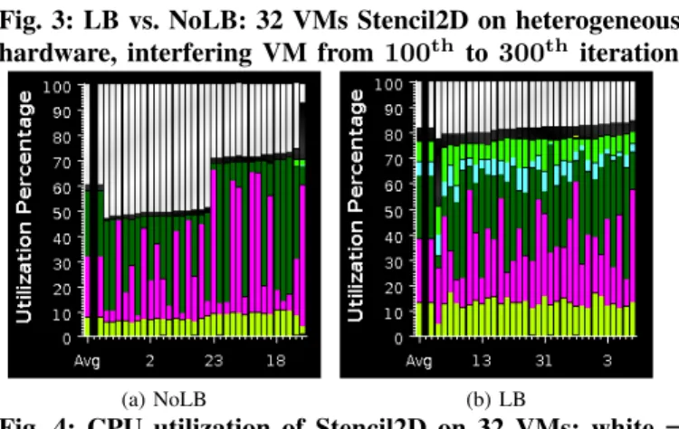
To understand the effect of our load balancer under hetero-geneity and interference, we ran 500 iterations of Stencil2D on 32 VMs (8 physical nodes – one Slow, rest Fast), and plotted the iteration time (execution time of an iteration) vs. iteration number in Figure 3. In this experiment, we started the job in interfering VM after 100 iterations of parallel job had completed. Load balancing was performed after every 20 steps, which manifests itself as spikes in the iteration time every
20th step. We report execution times averaged across three
runs and use wall clock time, which includes the time taken for object migration. The LB curve starts to show benefits as we reach 100 iterations, due to heterogeneity-aware load balancing. After 100 iterations, interfering job starts. When the load balancer kicks in, it restores load balance by redistributing tasks among VMs according to Algorithm 1. Now, there is a large gap between the two curves demonstrating the benefits of our refinement based approach, which takes around 3 load balancing steps to gradually reduce the iteration time after interference appears. The interfering job finishes at iteration 300 and hence the NoLB curve comes down. There is little reduction in LB curve, since the previous load balancing steps had reduced the impact of interference to a very small amount. The difference between the two curves after that is due to heterogeneity-awareness in load distribution.
To confirm that the achieved benefit is due to better load bal-ance, we used Projections [15] tool for performance analysis. Figure 4 shows the improvement in CPU (VCPU) utilization with load balancing for Stencil2D on 32 VMs, all running on Fast nodes in this case, with one interfering VM. In this Figure, y-axis represents CPU utilization, x-axis is (virtual) CPU number, with first bar as average. White portion (at top) represents idle time and colored portions (shaded) depict application functions. Black portion (below white) is overhead (see last processor in Figure 4a). The CPUs (x-axis) are sorted by the idle time using extrema analysis techniques. Observing Figure 4a, it is clear that there are 3 different clusters – 50%, 70%, and 90% utilization level. The difference between first two is due to the use of 2 types of processors. Though they have same processor frequency, the actual performance achieved is significantly different. There is very little load imbalance among processors in the same cluster, indicating that the distribution of work to processors is equal. The third cluster belongs to the VM which incurs interference. Figure 4b balances load. Here the idle time is due to the communication time, and is uniform across all CPUs. Overall, the average utilization increased from 60% to 82% using load balancing.
Next, we analyze the effect of few parameters on load bal-ancer performance followed by results for various applications.
0 0.05 0.1 0.15 0.2 0.25 0 50 100 150 200 250 300 350 400 450 500 Iteration time (s) Iteration number NoLB LB
Fig. 3: LB vs. NoLB: 32 VMs Stencil2D on heterogeneous hardware, interfering VM from 100th to 300th iteration
(a) NoLB (b) LB
Fig. 4: CPU utilization of Stencil2D on 32 VMs: white = idle time, black = overhead (including background load), colored portions = application functions, x-axis = VCPU. A. Analysis using Stencil2D
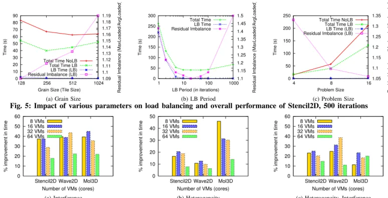
To achieve better understanding, we experimented with Stencil2d on 32 VMs (Fast processors, one interfering VM), and ran 500 iterations. We varied grain size, load balancing frequency and problem size. Here, we present our findings.
1) Effect of Grain Size and Overdecomposition: Grain size refers to the amount of work performed by a single task (object in Charm++ terminology). For Stencil2D, it can be represented by the matrix size of an object. Figure 5a shows the variation in execution time with object sizes. First, consider the NoLB case. As we decrease the grain size, hence increasing number of objects per processor, execution time decreases due to the benefits of overdecomposition: (a)better cache reuse by exploiting temporal locality and (b) hiding network latency through automatic overlap of computation and communication. After a threshold, time starts increasing, due to the overhead incurred by the scheduler and runtime for managing large number of objects. Hence, as we make objects very fine grained, performance degrades. Here, best performance is obtained with grain size = 512×512 elements.
The LB case (load balancing every 20 steps) introduces additional factors – (a) time spent in load balancing and (b)
load balancing quality, which affect the overall performance. From Figure 5a, we see that the total load balancing time (LB time), which includes time to make migration decisions and time spent in migrating objects, is negligible compared to the total time. However, LB time will be important as the compu-tation time decreases (e.g. strong scaling), and the ratio of LB time to compute time increases. For (b), we calculate
0 10 20 30 40 50 60 70 80 90 128 256 512 1024 1.09 1.1 1.11 1.12 1.13 1.14 1.15 1.16 1.17 1.18 1.19 Time (s)
Residual Imbalance (MaxLoaded/AvgLoaded)
Grain Size (Tile Size) Total Time NoLB
Total Time LB LB Time (LB) Residual Imbalance (LB)
(a) Grain Size
0 50 100 150 200 250 300 1 10 100 1000 1.1 1.15 1.2 1.25 1.3 1.35 1.4 1.45 1.5 Time (s)
Residual Imbalance (MaxLoaded/AvgLoaded)
LB Period (in iterations) Total Time LB Time Residual Imbalance (b) LB Period 0 50 100 150 200 250 4 8 16 1.05 1.1 1.15 1.2 1.25 1.3 1.35 Time (s)
Residual Imbalance (MaxLoaded/AvgLoaded)
Problem Size Total Time NoLB
Total Time LB LB Time (LB) Residual Imbalance (LB)
(c) Problem Size
Fig. 5: Impact of various parameters on load balancing and overall performance of Stencil2D, 500 iterations
0 10 20 30 40 50 60
Stencil2D Wave2D Mol3D
% improvement in time Number of VMs (cores) 8 VMs 16 VMs 32 VMs 64 VMs (a) Interference 0 10 20 30 40 50
Stencil2D Wave2D Mol3D
% improvement in time Number of VMs (cores) 8 VMs 16 VMs 32 VMs 64 VMs (b) Heterogeneity 0 10 20 30 40 50 60
Stencil2D Wave2D Mol3D
% improvement in time Number of VMs (cores) 8 VMs 16 VMs 32 VMs 64 VMs (c) Heterogeneity, Interference
Fig. 6: % benefits obtained by load balancing in presence of interference and/or heterogeneity for three different applications and different number of VMs, strong scaling
ageResidual Imbalance=M ax ComputeAvg Compute(+(+BackgroundBackground))LoadLoad
over all iterations and plot it on the same figure, with the right y-axis being the legend. We see that we get better load balance as we decrease object size, achieving residual imbalance of1.09for128×128. However, the best execution time is achieved for object size256×256due to the impact of additional factors, such as overhead. In general, we observed good load balance with degree of decomposition (ratio of objects to processors) >20.
2) Effect of Load Balancing Frequency: Next, we vary the load balancing frequency in the same setup, with fixed grain size of 256×256based on the results above. Figure 5b shows that the there is an optimal load balancing period. Very frequent load balancing (small LB period) results in most of the time being spent in making task migration decisions and migrating the data associated with objects, which degrades application performance. Moreover, it also results in lack of enough instrumented data for the load balancer to make intelli-gent decisions, leading to large residual imbalance. With very infrequent load balancing, such as LB period = 100 iterations, load balancer will be slow to adapt to the dynamic variations, leading to large residual imbalance. Hence, we settle for LB period = 20 iterations (which equals approximately 2 seconds here) except for runs on 64 VMs, where we used a period = 50 iterations. The optimal LB period depends on the iteration time and should be larger for small iteration time so that the gains achieved by improved load balance are not offset by time spent in balancing load.
3) Effect of Problem Size: Finally, we analyze the per-formance benefits for different problem sizes of same ap-plication – Stencil2D in the same setup, with fixed grain
size of 256 ×256 and LB period = 20. Figure 5c shows that the benefits increase with increasing problem size. With larger problem size, the computation granularity increases, reducing communication-to-computation ratio. Hence, any im-provement in computation time through load balancing will result in higher impact on the total execution time. Also, we get better load balance quality as we increase problem size – for 16K×16K matrix, we get residual imbalance of 1.05.
Application which are less communication-intensive are the most cloud-friendly one and are expected to be run in the cloud most because of better scalability. Also, the model expected to work better in cloud is weak scaling (same problem size per core with increasing cores) rather than strong scaling (same total problem size with increasing cores) [22]. In that context, our approach will be extremely useful for HPC in cloud.
B. Performance and Scalability of Three Applications To evaluate the robustness and efficacy of our load balancer in actual cloud scenario, we study three different cases (shown in Figure 6) – (a)Interference- one interfering VM, allFast nodes, (b)Heterogeneity – oneSlow node, hence fourSlow VMs, restFastand (c)Heterogeneity and Interference– one Slow node, hence four Slow VMs, rest Fast, one interfering VM (on aFast core) which starts at iteration 50. We ran 500 iterations for Stencil2D and Wave2D and 200 iterations for Mol3D, with load balancing every 20th step. We kept same
problem size while increasing number of VMs (strong scaling). Figure 6 shows that we achieve significant % reduction (=
TN oLB−TLB
TN oLB ×100) in execution time using load balancing
compared to the NoLB case, for different applications and different number of VMs under all three configurations. With
16 32 64 128 256 8 16 32 64 Time (s) Number of VMs (cores) Stencil2D Interf NoLB HeteroInterf NoLB Hetero NoLB 32 64 128 256 512 1024 8 16 32 64 Time (s) Number of VMs (cores) Wave2D HeteroInterf LB Hetero LB Interf LB 32 64 128 256 512 1024 8 16 32 64 Time (s) Number of VMs (cores) Mol3D Homo NoLB Ideal-Scaling (wrt to Homo 8 VMs)
Fig. 7: Scaling curves with and without load balancing in presence of interference and/or heterogeneity for three different applications, strong scaling
an interfering VM, we achieve up to 45% improvement in execution time (Figure 6a). The amount of benefits is different for different applications, especially in Figure 6b. We studied this behavior using Projections tool and found that our load balancer is distributing tasks well for all applications, but the difference in achieved benefits is due to the different sensitivity of these applications to CPU type and frequency. It can be inferred from Figure 6b that Mol3D is the most sensitive to CPU frequency, having most scope for improvement. Next, Figure 6c shows that our techniques are also effective in the presence of both the effects – the inherent hardware hetero-geneity and the heterohetero-geneity introduced by multi-tenancy.
Another observation from Figure 6 is the variation in the achieved benefits with increasing number of VMs. This is attributed to the tradeoff between two factors:(1)Since there is only one VM sharing physical CPU with interfering VM, running on larger number of VMs implies distributing the work of the overloaded VM to an increasing number of underutilized VMs, which results in larger reduction in execution time (e.g. Figure 6a Mol3D, 8 VM vs. 16 VM). (2) As we scale, the average compute load per VM decreases. Hence, other factors, such as communication time, dominate the total execution time. This implies that even with better load balance and higher % reduction in compute time, overall benefit is small, since communication time is unaffected. Hence, as we scale further, benefits decrease, but they still remain substantial.
Moreover, as we scale, benefits can actually be more impor-tant because we save across larger number of processors. As an example, from Figure 6b Stencil2D, we save 18.8% over 32 VMs, with absolute savings = 32×0.188×48.09 = 289.28
CPU-seconds, where application took 48.09 seconds on 32 VMs. Juxtaposing this with 20.5% reduction in time over 16 VMs which results in absolute savings= 16×0.205×86.77 = 284.32CPU-seconds, where application took 86.77 seconds on 16 VMs, we see that the overall savings are more for 32 VM case compared to 16 VMs. Also, since we achieve higher % benefits with larger problem sizes (Section VI-A3, Figure 5c), the benefits will be even higher for weak scaling compared to strong scaling as the impact of factor 2 above is minimized.
The primary objective of running in parallel is to get reduced execution time with increasing compute power. However, it is not clear from Figure 6 whether we achieve that goal. Hence, we plot execution time vs. number of VMs for same
experi-ments, as shown in Figure 7. For the purpose of comparison, we also include the runs without any interfering VMs, with all VMs mapped toFastnodes (Homocurve in Figure 7). Figure 7 shows that our load balancer brings the NoLB curves down and close to the Homo curve. At some data points, the LB curves are below the homo curve, since even the Homo curves can benefit from load balancing (shown earlier in Figure 4 that application performance on two types ofFast processors is somewhat different). The superlinear speedup achieved in some cases can be attributed to better cache performance.
The scale of our experiments was limited by the availability of nodes in our cloud setup since we needed administrative privileges from provider perspective. However, we believe that our techniques will be equally applicable to larger scales since the effectiveness of similar load balancing strategies have been demonstrated on large-scale supercomputer applications [23].
VII. RELATEDWORK
There have been several studies on evaluation of HPC in cloud (mostly on Amazon EC2 [1]) using benchmarks (such as NPB) and real world applications [2–5]. These studies have concluded that even though cloud can be potentially more cost-effective than supercomputers for some HPC applications, there are challenges that need to be addressed to enable effi-cient use of clouds for HPC. Some challenges are insuffieffi-cient network and I/O performance in cloud, resource heterogeneity, and unpredictable interference arising from other VMs.
The approaches taken to reduce the gap between traditional cloud offerings and HPC demands can be classified into two broad categories – (1) those which aim to bring clouds closer to HPC and (2) those which want to bring HPC closer to clouds. Examples of (1) include HPC-optimized clouds such as Amazon Cluster Compute [6] and DoE’s Magellan [4]. An-other area of research in (1) is making cloud schedulers (VM placement algorithms) aware of the underlying hardware and the nature of HPC applications. Examples include the work by Gupta et al. [8] and OpenStack community towards making OpenStack scheduler architecture-aware [7]. Related work on modifying the scheduling in virtualization layer include VM prioritization and co-scheduling of co-related VCPUs [24]. The latter approach (2) has been relatively less explored. Fan et al. proposed topology aware deployment of scientific appli-cations in cloud, and mapped the communication topology of an HPC application to the VM physical topology [9].
In this work, we took the latter approach and explored whether we can make HPC applications more cloud friendly using a customized parallel runtime system. We built upon our earlier work [10] where we proposed similar load balancing for addressing background loads. This work extends previous work in multiple ways – First, in [10], we assumed that we can get accurate compute time for tasks, that is independent of the background load. However, in cloud, it may not be possible to separate the time taken by background load from application load since virtualization hides the presence of time-sharing of physical nodes among VMs. Secondly, we make the load balancer aware of both – hardware heterogeneity and multi-tenancy in cloud. Thirdly, we evaluate our techniques on an actual cloud with VMs whereas in the earlier work, we did not consider effects of virtualization. Brunner et al. [25] proposed a load balancing scheme similar to ours but in the context of workstations. Our work differs from theirs in the same ways as above. Moreover, our scheme uses a refined load balancing algorithm that reduces number of task migrations.
VIII. CONCLUSIONS, LESSONS ANDFUTUREWORK In this paper, we presented a load balancing technique which accounts for heterogeneity and interfering VMs in cloud and uses object migration to restore load balance. Experimental results on actual cloud showed that we were able to reduce execution time by up to 45% compared to no load balancing. The lessons learned and insights gained are summarized as:
• Heterogeneity-awareness can lead to significant perfor-mance improvement for HPC in cloud. Adaptive parallel runtime system are extremely useful in that context. • Besides the static heterogeneity, multi-tenancy in cloud
introduces dynamic heterogeneity, which is random and unpredictable. The overall effect being poor performance of tightly-coupled iterative HPC applications.
• Even without the accurate information of the nature and amount of heterogeneity (static and dynamic but hidden from user as an artifact of virtualization), the approach of periodically measuring idle time and migrating load away from time-shared VMs works well in practice. • Tuning the parallel application for efficient execution in
cloud is non-trivial. Choice of load balancing period and computational granularity can have significant impact on performance but the optimal values depend on application characteristics, size, and scale. Runtime systems which can automate the selection and dynamic adjustment of such decisions will be increasingly useful in future. We believe that some of our approaches and analysis can also be leveraged for future exascale applications and runtimes. According to an exascale report, one of the Priority Research Direction (PRD) for exascale is to “develop tools and runtime systems for dynamic resource management” [26].
In future, we plan to extend our load balancer such that data migration is performed only if we expect gains that can offset the cost of migration. Also, we will explore the use of VM steal cycles, where supported. We have demonstrated that our techniques work well with iterative applications, and when the
external noise is quite regular. In future, we plan to explore the cases when the interference is irregular, such as fluctuating loads of web applications. Finally, we plan to evaluate our techniques on a larger scale – on an actual cloud, if available in future, or through simulated or emulated environment.
ACKNOWLEDGMENTS
This work was supported by HP Labs’ 2012 IRP award.
REFERENCES
[1] “Amazon Elastic Compute Cloud,” http://aws.amazon.com/ec2. [2] E. Walker, “Benchmarking Amazon EC2 for High-Performance
Scien-tific Computing,”LOGIN, pp. 18–23, 2008.
[3] A. Iosup et al., “Performance Analysis of Cloud Computing Services for Many-Tasks Scientific Computing,” Parallel and Distributed Systems,
IEEE Transactions on, vol. 22, no. 6, pp. 931 –945, june 2011.
[4] “Magellan Final Report,” U.S. Department of Energy (DOE), Tech. Rep., 2011, http://science.energy.gov/∼/media/ascr/pdf/program-documents/
docs/Magellan Final Report.pdf.
[5] A. Gupta and D. Milojicic, “Evaluation of HPC Applications on Cloud,”
inOpen Cirrus Summit (Best Student Paper), Atlanta, GA, Oct. 2011,
pp. 22 –26. [Online]. Available: http://dx.doi.org/10.1109/OCS.2011.10 [6] “HPC on AWS,” http://aws.amazon.com/hpc-applications.
[7] “Nova Scheduling Adaptations,” http://xlcloud.org/bin/download/ Download/Presentations/Workshop 26072012 Scheduler.pdf.
[8] A. Gupta, L. Kale, D. Milojicic, P. Faraboschi, and S. Balle, “HPC-Aware VM Placement in Infrastructure Clouds ,” inIEEE Intl. Conf. on
Cloud Engineering IC2E ’13, march. 2013.
[9] P. Fan, Z. Chen, J. Wang, Z. Zheng, and M. R. Lyu, “Topology-Aware Deployment of Scientific Applications in Cloud Computing,” Cloud
Computing, IEEE International Conference on, vol. 0, 2012.
[10] O. Sarood, A. Gupta, and L. V. Kale, “Cloud Friendly Load Balancing for HPC Applications: Preliminary Work,” inParallel Processing
Work-shops (ICPPW), 2012 41st Intl. Conf. on, sept. 2012, pp. 200 –205.
[11] L. Kale and S. Krishnan, “Charm++: A Portable Concurrent Object Oriented System Based on C++,” inOOPSLA, September 1993. [12] L. V. Kale and G. Zheng, “Charm++ and AMPI: Adaptive Runtime
Strategies via Migratable Objects,” inAdvanced Computational
Infras-tructures for Parallel and Distributed Applications, M. Parashar, Ed.
Wiley-Interscience, 2009, pp. 265–282.
[13] “MPI: A Message Passing Interface Standard,” inM. P. I. Forum, 1994. [14] A. Avetisyan et al., “Open Cirrus: A Global Cloud Computing Testbed,”
IEEE Computer, vol. 43, pp. 35–43, April 2010.
[15] L. Kal´e and A. Sinha, “Projections : A Scalable Performance Tool,” in
Parallel Systems Fair, Intl. Parallel Processing Sympos ium, Apr. 1993.
[16] “NAS Parallel Benchmarks,” http://www.nas.nasa.gov/Resources/ Software/npb.html.
[17] A. Bhatele, S. Kumar, C. Mei, J. C. Phillips, G. Zheng, and L. V. Kale, “Overcoming Scaling Challenges in Biomolecular Simulations across Multiple Platforms,” inIPDPS 2008, April 2008, pp. 1–12.
[18] “OpenStack Cloud Computing Software,” http://openstack.org. [19] “KVM – Kernel-based Virtual Machine,” Redhat, Inc., Tech. Rep., 2009. [20] A. J. Younge et al., “Analysis of Virtualization Technologies for High Performance Computing Environments,”Cloud Computing, IEEE Intl.
Conf. on, vol. 0, pp. 9–16, 2011.
[21] A. Gupta, D. Milojicic, and L. Kale, “Optimizing VM Placement for HPC in Cloud,” inWorkshop on Cloud Services, Federation and the 8th
Open Cirrus Summit, San Jose, CA, 2012.
[22] T. Sterling and D. Stark, “A High-Performance Computing Forecast: Partly Cloudy,”Computing in Sci. and Engg., pp. 42–49, Jul. 2009. [23] G. Zheng, “Achieving High Performance on Extremely Large Parallel
Machines: Performance Prediction and Load Balancing,” Ph.D. disser-tation, Dept. of CS, Univ. of Illinois at Urbana-Champaign, 2005. [24] O. Sukwong and H. S. Kim, “Is co-scheduling too expensive for smp
vms?” ser. EuroSys ’11. NY, USA: ACM, 2011, pp. 257–272. [25] R. K. Brunner and L. V. Kal´e, “Adapting to Load on Workstation
Clusters,” in 7th Symposium on the Frontiers of Massively Parallel
Computation. IEEE Computer Society Press, Feb. 1999, pp. 106–112.
[26] D. Brown et al., “Scientific Grand Challenges: Crosscutting Technolo-gies for Computing at the Exascale.” U.S. DOE PNNL 20168, Report from Workshop on Feb. 2-4, 2010, Washington, DC, Tech. Rep., 2011.