Chapter 2
A Strong Motion Velocity Meter in a
Modern Seismic Network?
2.1
Introduction
Seismometry has seen huge advances in the past 30 years. The dynamic range of typical seismometers has increased from less than 5 orders of magnitude to more than 7, pri-marily because of the development of force feedback systems (Wielandt and Streckeisen, 1982; Iwan et al., 1985; Wielandt and Steim, 1986). Advances in recording systems have been even more dramatic; current 24-bit digitisers record over 7 orders of magnitude com-pared to the 3 orders of magnitude achievable by analogue recording devices (Trifunac and Todorovska, 2001a). The past 30 years have also seen the dramatic development of digital data communication, processing and storage, which has prompted the development of a plan for an Advanced National Seismic Plan (Heaton et al., 1989; Benz and Filson, 1998). These new capabilities allow us to devise new strategies to record ground motions. One such strategy, whose advantages are the subject of this Chapter, would be to deploy con-tinuously telemetered strong motion velocity seismometers in place of existing triggered strong motion accelerometers.
The most critical role of strong motion networks is to provide on-scale recordings of potentially damaging motions over a broad frequency band. Because continuous analogue recording is extremely expensive and strong shaking is infrequent, strong motion seismo-graphs were designed to record only during strong ground shaking. Furthermore, because of the limited dynamic range of recording devices, it was most efficient to record ground ac-celeration, since near-source strong ground motions have relatively flat acceleration spectra in the band from 0.3 to 3.0Hz.
The typical station specifications for a modern digital network are described, using the California Integrated Seismic Network, CISN, as an example. A CISN station
con-as an STS-2 or a CMG-40T, and a strong motion accelerometer, such con-as an FBA-23, or EpiSensor. These instruments record on a 24-bit digitiser that has continuous, near-real-time telemetry of high sampled data (80-100sps) to the CISN centre at Caltech and USGS-Pasadena.
The main thrust of this Chapter is to discuss whether it would be better to deploy a velocity-recording strong motion instrument in place of existing force-balance accelerom-eters. Using a large suite of real Earth signals, the hypothetical long-period low-gain ve-locity seismometer (with a clipping level set to ±5m/s) is compared to the existing ±2g clipping Kinemetrics FBA-23 accelerometer.
It is shown that there are significant advantages in the deployment of the proposed instrument over an accelerometer —
•The velocity instrument would have several orders of magnitude greater sensitivity in the period band from 2sto several hundred seconds. This would allow the recording of
— long-period basin response from regional earthquakes as small as M3.0, and — teleseismic ground motions from earthquakes as small as M6,
which could potentially lead to dense spatial recording of small amplitude motions that are not recorded by traditional strong motion networks.
• Furthermore, as well as allowing full recovery of ground acceleration, recovery of ground displacement is likely to be more stable from such a long-period low-gain broad-band seismometer.
It is anticipated that a strong motion velocity seismometer would essentially be a low-gain version of existing broadband seismometers, such as the Weilandt-Streckeisen STS-2, and thus its cost would likely be similar to other broadband seismometers. Unfortunately, so would its size and weight. Thus the clear advantages would be offset by significantly poorer cost, size and weight than an accelerometer, which makes it somewhat unwieldy for dense building instrumentation.
At this stage it is pertinent to discuss the design of such an instrument. The STS-2 is designed to respond as a simple single degree of freedom oscillator with free period of 120s, with differential feedback, and so has output proportional to ground velocity from
120sto high frequencies. In reality, it consists of a mechanical pendulum with free period of 2s. The feedback electronics produce a heavily over-damped (∼1000% of critical) output, and so the suspension displacement is proportional to ground velocity over a wide frequency band about this free period. Chapter 3 presents an investigation into a relatively new Japanese strong motion velocity recording sensor, the VSE-355G2. This instrument has a mechanical pendulum of about 3Hzwith a similar feedback system. Unfortunately it is also slightly heavier (20kg), and larger (30cmx 30cmplan x 20cmhigh) than the STS-2. A strong motion velocity seismometer could record a broader swath of Earth motions than are currently recorded by existing strong motion accelerometers. With a clipping level of±5m/s (a velocity magnitude greater than that of any seismic ground motion measured to date) it would recover on-scale all motions relevant to structural engineering, and it would record long-period motions with accelerations too small to be recorded by traditional accelerometers. It is estimated that direct recording of velocity with a dynamic range of 140dBwould permit recording of broadband motions from regional and near-source events as small as M3.0. These broadband motions could be used to study path effects such as the amplification of long-period motions by basins. In addition, a strong motion velocity array should be capable of recording teleseisms as small as M6. This could lead to dense spatial recording of small amplitude motions that are not recorded by traditional strong motion networks.
Single differentiation of the raw velocity output would produce the acceleration records currently used by engineers. However, the real issue is not acceleration versus velocity, but is one of having accurate motion in the frequency band of interest. The velocity seismome-ter has the significant advantage that displacement estimates of ground motion would be obtained from a single integration of the raw data. Current strong motion velocity devices have flat responses up to 70Hz, so acceleration timeseries can be recovered up to this fre-quency, which is satisfactory for most engineering purposes, as few structures are damaged by energy at 70Hz. Further, as long as the longest frequencies in a signal are below the low frequency corner of the instrument (∼100s— in effect excluding all but static offsets), sin-gle integration would result in smaller long period error than would a double integration, assuming a similar error in the true signal of velocity and acceleration. Single integration
regard to static offsets. Even very small baselines or linear trends, which are difficult to isolate and remove in current strong motion records, can seriously distort the resultant dis-placement after double integration, often leaving its estimation more a matter of judgment rather than science (Boore, 2001). Resolving long-period motions associated with static displacements is somewhat more complicated, as will be discussed in Chapters 3 and 4. Essentially, as the instrument response of the strong motion sensor needs to be removed to recover the zero frequency static offset, the strong motion velocity meter provides no im-provements over traditional accelerometers for this. As the velocity meter is also an inertial seismometer like the accelerometer, the sensor is also very sensitive to tilt. Small changes in tilt can significantly affect the derivation of ground displacement, as pointed out by Tri-funac and Todorovska (2001b). In order to fully derive the translational displacements in the presence of tilt requires additional information from a co-located rotational meter, or a nearby true displacement meter, such as GPS.
The increased range of Earth recordings obtained from using the proposed strong mo-tion velocity seismometer is demonstrated through comparisons of signal recovery with both a typical accelerometer, the Kinemetrics FBA-23, and a broadband velocity instru-ment, the Weilandt-Streckeisen STS-2. The performance of each device is illustrated by showing how their dynamic characteristics relate to a wide range of seismic motions, in terms of frequency content and acceleration amplitude. An in-depth description of the components of the complete seismographic system — which includes a digital recording device as well as the seismometer — and how the dynamic range is finally determined, is first presented.
2.2
A Typical CISN Station
The California Integrated Seismic Network (CISN),www.cisn.org, is the network source of most of the data used not only in this Chapter, but throughout the thesis. The CISN col-lates data from the Southern California Seismic Network (SCSN), the Northern California Seismic Network (NCSN), and many strong motion networks around the State of
Califor-nia. Data is available from the individual network data centre Web portals: the Southern California Earthquake Data Center (SCEDC),www.scecdc.scec.org, the Northern Cal-ifornia Earthquake Data Center (NCEDC),quake.geo.berkeley.edu, and the Consor-tium of Organizations for Strong Motion Observation Systems (COSMOS) Strong Motion Virtual Data Center,www.cosmos-eq.org. CISN is a recent amalgamation of the three ex-isting organisations. Most data herein is from the SCSN. This network has immensely ben-efited from the TriNet project (1997-2001). TriNet provided a dense, modern seismic infor-mation system for Southern California (Hauksson et al., 2001; Hauksson et al., 2003), with over 150 broadband stations. TriNet itself grew out of the first digital, co-ordinated broad-band and strong motion seismic network in Southern California, TERRAscope (Kanamori et al., 1991), which comprised 28 stations.
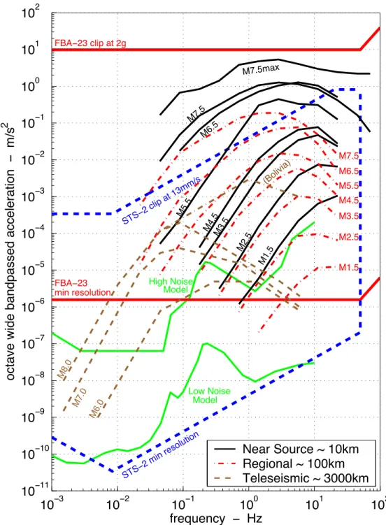
The SCSN is designed to record on-scale motions from an M8 earthquake, as well as large teleseismic earthquakes and small regional motions. The entire network has a minimum earthquake detectability threshold of M1.8. This requires not only an even and relatively dense distribution of stations, but each station must also have a very large dy-namic range, of about 10 orders of magnitude, or 200dB. Thus the typical station consists of two broadband force-balance seismometers, typically a high-gain velocity recording de-vice, such as an STS-2 or a CMG-40T, and a low-gain strong motion accelerometer, such as an FBA-23, or EpiSensor. These instruments record on a 24-bit Quanterra digitiser — about 7 orders of magnitude dynamic range, or 138dB. A plot of the dynamic range of the typical sensor/datalogger configuration is in Figure 2.1, which also includes the average size of earthquake signals from events of various magnitudes and distances. A detailed explanation of how this plot was produced is in Sections 2.4 and 2.5. The digitiser has continuous, near-real time telemetry of high sampled data (80−100sps) to the data pro-cessing and archiving centres at the Caltech Seismological Lab, located in the South Mudd Laboratory at Caltech, and across the road from South Mudd, at the USGS Pasadena office, 525 S. Wilson Ave. The digitisers can also log the continuous (in a 3-week buffer) and triggered data locally in the event of a transmission breakdown.
The data processing centres receive continuous data from more than 1200 high sam-ple channels (100sps, 80sps), and over 2000 lower samsam-ple channels (20sps, 1sps, 0.1sps,
10−3 10−2 10−1 100 101 102 10−11 10−10 10−9 10−8 10−7 10−6 10−5 10−4 10−3 10−2 10−1 100 101 10 High Noise Model Low Noise Model STS− 2 clip at 13mm/s STS− 2 min resolution FBA−23 clip at 2g FBA−23 min resolution M7.5max M7.5 M6.5 M5.5 M4.5M3.5 M2.5 M1.5 M7.5 M6.5 M5.5 M4.5 M3.5 M2.5 M1.5 M8.0 (Bolivia) M7.0 M6.0 frequency − Hz
octave wide bandpassed acceleration
− m/s 2 Near Source ~ 10km Regional ~ 100km Teleseismic ~ 3000km
Figure 2.1: Frequency - amplitude plot for octave wide bandpasses of ground motion accel-eration. A typical CISN station records all motions located between the FBA-23 clip and the STS-2 minimum resolution, encompassing the ∼10 orders of magnitude required to cover the Earth’s signals. Assumes 24-bit digitiser. Note that instrument limits are scaled down to account for the bandpassing of the event data. Ground motions recorded on-scale by the FBA-23 lie between the thick solid lines. The thick dashed lines give the dynamic range of the STS-2. Noise levels are the USGS High and Low Noise Models (Peterson, 1993).
health monitoring channels).
In certain cases, especially for stations in noisy areas, such as buildings, only a strong motion accelerometer is deployed with the 24-bit digitiser. This is the case at many of the stations around Caltech Campus, such as the Millikan Library (MIK), the Broad Center (CBC) and the USGS Building (GSA). Some other stations, such as the Caltech Athenaeum (CAC), have only an accelerometer alongside a 19-bit K-2 digitiser.
Other remote stations may only have a short period Mark Products L4-C vertical instru-ment with limited dynamic range of about 55dB, primarily used for earthquake detection and location.
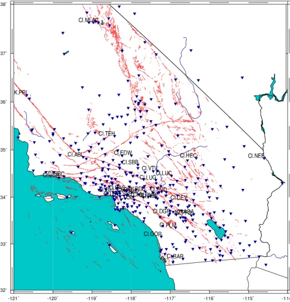
In total the SCSN currently has about 155 stations with both broadband and strong motion sensors, with about 55 stations with a single 3-component strong motion sensor. There are also about 140 stations with vertical component short period sensors only. A station location map for the entire SCSN is in Figure 2.2, and Figure 2.3 is a close up of the LA basin.
The data is stored in both a continuous format, at 20sps, and in triggered ‘event’ format, at 80-100sps, at the Southern California Earthquake Data Center, SCEDC. The digitisers are all Quanterra models, the older dataloggers have a maximum sampling rate of 80sps, the new models 100sps. Triggered event data is available a few hours after an event is identified, and continuous data for the previous day is made available at 12AM GMT.
Summary tables of typical instruments and digitisers are in Tables 2.1 and 2.2. The instrument response for the broadband sensors is in Figure 2.4. The broadband instrument response is flat to velocity for all the instruments from about 7Hz (the other instruments have their high frequency cutoff all beyond 20Hz) to 30sand further, up to 360s. Beyond the long-period period corner, all sensors have a drop-off at a rate of −12dB/oct to ve-locity, which means in this recording range, the instruments are flat to the differential of acceleration (the ‘jerk’). At frequencies less then the high frequency cutoff, these instru-ments all respond essentially as single degree of freedom (SDOF) simple oscillators with differential feedback.
Data is available via a Web browser at www.scecdc.scec.org/stp.html, or from a stand-alone software version on the users computer, downloadable fromwww.scecdc.
Figure 2.2: Southern California Seismic Network (SCSN) station map. Known faults are in light shade. A selection of station names is shown.
Figure 2.3: Southern California Seismic Network (SCSN) station map for the Los Angeles basin. Known faults are in light shade. CI.PAS is station at Kresge Lab., Pasadena.
Manufacturer Type Freq. Range Sensitivity Clip Level
High Gain Broad-Band Seismometers :
Streckeisen STS-1 0.0027-10Hz 2500V/m/s(vert) ∼0.8cm/s 2300V/m/s(horiz) ∼0.8cm/s Streckeisen STS-2 0.0083-50Hz 1500V/m/s 1.3cm/s Guralp CMG-1T 0.0027-10Hz 1500V/m/s ∼1cm/s Guralp CMG-40T 0.033-50Hz 800V/m/s ∼1cm/s Guralp CMG-3ESP 0.0083-50Hz 2000V/m/s ∼1cm/s Guralp CMG-3T 0.0083-50Hz 1500V/m/s ∼1cm/s Low Gain Broad-Band (Accelerometer/Strong Motion Velocity) :
Kinemetrics FBA-23 DC-50Hz 5V/g 2g Kinemetrics EpiSensor DC-180Hz 10V/g 2g Tokyo-Sokushin VSE-355G3 ∼.01-70Hz 10V/m/s ∼200cm/s Table 2.1: Summary of typical instruments used in the California Integrated Seismic Net-work. Abridged from Hauksson et al. (2001)
105 106 107 108 109 101 0 0.001 0.01 0.1 1 10 100 STS-1 STS-2 CMG3ESP CMG40T
V
e
lo
c
it
y
R
e
s
p
o
n
s
e
,
c
o
u
n
ts
/(
m
/s
)
Frequency (Hz)
-4 -3 -2 -1 0 1 2 3 4 0.001 0.01 0.1 1 10 100 STS-1 STS-2 CMG3ESP CMG40TP
h
a
s
e
R
e
s
p
o
n
s
e
(
ra
d
ia
n
)
Frequency (Hz)
(a)
(b)
Figure 2.4: Response for typical broadband CISN instruments (from Hauksson et al. (2001)).
Manufacturer Type Site Recording Channels Max. SPS Volts/cts Quanterra Q980 1.6Gb 9 80 20/223 Quanterra Q380 1.6Gb 3 80 20/223 Quanterra Q680 1.6Gb 6 80 20/223 Quanterra Q4128 1.6Gb 8 100 20/223 Quanterra Q730 1.6Gb 6 100 16/223 Quanterra Q730E 280Mb 6 100 16/223 Quanterra Q330 20Gb 6 200 20/223 Kinemetrics K2 64Mb 4 100 2.5/223 Table 2.2: Summary of typical digitisers used in the California Integrated Seismic Network. Abridged from Hauksson et al. (2001)
scec.org/ftp/programs/stp. This later version can be opened using perl scripts for automated searching and downloading of data.
2.3
The Definition of Dynamic Range
Following Heaton (2003), the dynamic range,DR, of an instrument is defined as the ratio of the largest on-scale/linear measurement, Mmax divided by the smallest measurement
resolvable by the instrument,Mmin:
DR= Mmax
Mmin (2.1)
In the context of seismic instrumentation, the measurement is usually voltage output for a seismometer, or counts for a digitiser.
Traditionally, dynamic range is given in the units of decibels (dB), 101th of a Bel. A Bel is defined as a base 10 logarithmic measure of energy per unit time, or power. Since the power of a signal is proportional to the square of the signal amplitude:
DRdB = 10log10 ! Mmax Mmin "2 dB (2.2) = 20log10 ! Mmax Mmin " dB (2.3)
largest motions from large earthquakes to the noise levels at the quietest sites (such as recorded at depth in a mine shaft in a seismically inactive region far from the ocean). Thus the dynamic range of the Earth is:
DRdB(Earth) = 20log10 ! 1010 1 " dB (2.4) = 200dB (2.5)
Similarly,morders of magnitude dynamic range is equivalent to (20∗m)dB.
Seismic recordings made on traditional recording paper have a maximum amplitude of about 10cm, and a minimum resolution of about 0.1mm. This is a dynamic range of 3 orders of magnitude, or 60dB.
Modern seismometers record on digital recorders, which convert the analogue voltage seismometer output to digital counts. The nominal dynamic range is determined by the number of bits used to characterise the voltage. One bit is used to determine whether the signal is positive or negative, and each additional bit represents a factor of 2 in dynamic range, so dynamic range is 2n−1. For a 24-bit digitiser, the dynamic range is 223or 8388608. This is 138.5dB, or 138.5dB/20∼7 orders of magnitude.
[An alternative, quick way to determine the dynamic range of a digitiser in dB is DRdB= (#bits−1)∗6.02, as each additional bit increases the dynamic range by 20log(2) =
6.02.]
2.4
The Seismographic System
The range of amplitude and frequency recorded by a modern seismographic system is con-trolled by both the seismometer and the digitiser, or digital recorder. Ideally, the maximum gain of the datalogger (2(n−1)counts for a n-bit system) should be reached when the in-strument is at its clip level. If so, the minimum resolution of the seismographic system is determined by lowest resolution of the instrument and digitiser. Thus, the dynamic range
of the 2 components is investigated separately, to fully understand the dynamic range of the complete system.
Similarly, the behaviour of a system at clipping is dependent on the clipping charac-teristics of both the datalogger and sensor. With regards to the datalogger, many n-bit instruments simply cannot measure/output any more then 2n−1 counts, and will flat-line if the input signal is larger than this. Modern Quanterra 330 series instruments are in fact 27-bit sensors, though linearity of signal output is only guaranteed up to 24-bit. Thus the output can measure above 223 or 8,388,608 counts. Similarly, the instruments manufactur-ers design the instruments only to guarantee linearity up to the advertised clip level. Once this has been exceeded, a range of signal errors can occur, ranging from the relatively in-nocuous (and this very difficult to recognise as incorrect) small drift away from linearity, to spikes, flat-lines and long-period instrument responses. Many of these will be observed in practice in the subsequent Chapters.
2.4.1
Dynamic Range of the Digital Recorder
Current state-of-the-art digital recorders employ 24-bit digitisers. The nominal dynamic range of such a device is about 140dB. Theoretically, the dynamic range can exceed 140dB at low frequencies, since low frequency signals are oversampled and each point is the av-erage of many samples. However, this dynamic range enhancement does not occur where the noise is characterised by a power density that increases as frequency decreases, i.e., some form of 1/f noise. This type of noise has a constant power in frequency bands of equal relative width (Wielandt and Streckeisen, 1982). Most electronic systems, in fact, are characterized by 1/f noise below 1Hz, and hence no resolution enhancement occurs (Joe Steim, personal communication, 2001). In practice, under normal operating temperatures, the dynamic range can indeed increase. For example, the Quanterra Q330, with 135dB nominal dynamic range, at 26◦C records 136dB at 10Hz, up to 142dB at 0.5Hz, before dropping slightly at lower frequencies (Joe Steim, personal communication, 2001). As this is not a very large difference, I will assume, for the purposes of this work, a frequency-independent constant dynamic range of 140dB, approximately 7 orders of magnitude, for
2.4.2
Dynamic Range of Each Seismometer
— FBA-23The clipping limit of the FBA-23 seismometer is ±19.6m/s2 (±2g) up to its corner fre-quency of 50Hz. By comparing ground motions recorded simultaneously with the FBA-23 and STS-2, it was established that the FBA-23 can resolve acceleration above the noise level of the instrument down to about 3x10⁻⁶m/s2 across a broad band of frequencies (0.01 to 10Hz). This is illustrated in Figures 2.13 and 2.14, from Section 2.5, which show the bandpassed records of a M8.1 event at 2900kmepicentral distance. The FBA-23 noise at periods of about 100s and 50sare both of this level. For example, in Figure 2.14, the noise level is approximated as a sine wave with a 100speriod and amplitude 5x10⁻⁵m/s:
˙
unoise = 5x10⁻⁵sin 2πfτ m/s
= 5x10⁻⁵sin(6.28x10⁻²)τ m/s
⇒u¨noise = 3.14x10⁻⁶cos(6.28x10⁻²)τ m/s2
and thus the amplitude of this wave in acceleration is approximately 3.14x10⁻⁶m/s2, 136dBbelow the clip level of±19.8m/s2. This is less than the published 145dBfor the fre-quency range 0.01 to 20Hz(www.kinemetrics.com), but could also be due to limitations of the digitiser.
Further evidence for this noise level can be seen in Figure 2.5. In this plot, real con-tinuous ambient noise data from a selection of accelerometer/digitiser configurations in the SCSN is presented. On average, FBA channels record noise at about 136dBbelow the clip level, whilst the EpiSensor has a better dynamic range, nearer 140dB. This general trend, with a relatively constant amplitude over a wide band-width, occurs for a variety of sta-tions and digitisers, which indicates this observed noise line is the actual noise floor of the instrument, rather than station’s local site noise, or digitiser noise.
ac-10−3 10−2 10−1 100 10−8 10−7 10−6 10−5 FBA at PAS STS−2 at PASB VSE at PASB GSC SVD USC DJJ ALP THX frequency − Hz
octave wide bandpassed acceleration
−
m/s
2
Expected 136dB min for FBA
Expected 140dB min for EPI
USC FBA Q980 THX FBA Q4128 GSC FBA Q4120 SVD FBA Q680 DJJ EPI Q4120 ALP EPI Q680
Figure 2.5: Comparison of noise floors for various accelerometer/digitiser configurations deployed in SCSN. All station data from a 3hour period on 1 April 2002. Also includes data from test station PASB, which at the time of the comparison, housed a Japanese Strong Motion Velocity Meter, the VSE-355G2, and an STS-2. PAS and PASB are essentially co-located.
— STS-2
Broadband seismometers such as the STS-2 have more complex characteristics. For seis-mic signals with periods shorter than the corner frequency (120sfor an STS-2), they typ-ically have clip levels that are given in both velocity and acceleration; in the case of the STS-2 this is ±13mm/s and ±3.3m/s2 (±0.34g). Velocity clip levels are often given as peak-to-peak values, for the STS-2 this would be 26mm/s peak-to-peak, hence the 1/2 peak-to-peak value is 13mm/s. The minimum resolvable motion for the STS-2 is not a simple function, or indeed directly related to the clip; in fact it is highly dependent on frequency, and is greater than 140dB for the frequency range of interest. The instrument noise level is published in the STS-2 manual (Streckeisen and Messgerate), and is shown in Figure 2.6.
— Strong Motion Velocity Meter
The hypothetical long-period, low-gain velocity instrument would have a similar type of re-sponse as the STS-2, with a corner frequency at 120s, and clip level at±5m/sand±49m/s2 (±5g). Minimum resolution is assumed to be 140dBbelow the clip level, a similar value to both the STS-2 and FBA-23.
The dynamic characteristics of these three seismometers are summarised in Table 2.3, and illustrated in Figure 2.6.
Instrument Type Free Period Clip Level
FBA-23 0.02s (50Hz) ±19.6m/s2(±2g)
STS-2 120s (0.0083Hz) min[±13mm/s,±3.3m/s2(±0.34g)]
strong motion velocity 120s (0.0083Hz) min[±5m/s,±49m/s2(±5g)]
Table 2.3: Comparison of important properties of the instruments
The final response of the seismographic system is similar to the instrument response, but the system dynamic range at any frequency does not exceed 140dBdue to the limitations
10
−310
−210
−110
010
110
210
−1210
−1010
−810
−610
−410
−210
010
2High Noise Model
Low Noise Model
FBA
−
23 clip at 2g
FBA
−
23 min resolution
Velocity Meter clip at 5m/s / 5g
Velocity Meter min resolution
STS
−
2 clip at 13mm/s
STS
−
2 min resolution
frequency
−
Hz
acceleration
−
m/s
2Figure 2.6: Instrument responses in terms of acceleration. Dashed lines indicate regions of uncertain instrument response. For the FBA-23 and STS-2, dotted lines indicate areas 140dBbelow instrument clipping levels. Noise levels are the USGS High and Low Noise Models (Peterson, 1993).
is affected.
Note that for brevity and simplicity, hereafter the combined seismographic system com-prising both the instrument and digitiser is referred to simply as the ‘instrument’ or the ‘seismometer’.
2.5
Strong Motion Instrument Comparisons Using Recorded
Earthquake Signals
The hypothetical strong motion velocity meter is compared with the Kinemetrics FBA-23 accelerometer, and the Weilandt-Streckeisen STS-2 broadband velocity seismometer. To show the range of motions typically recorded on-scale and above the instrument noise of each instrument, their performance in frequency and amplitude of acceleration is plotted in relation to a broad range of Earth signals typically of interest to engineers and seismol-ogists. Measured signal strengths of each record are not power spectra of the broadband time series, but discrete octave-wide bandpasses. This allows the inconsistencies in the power spectra associated with arbitrarily picking a duration for the transient earthquake signals (Aki and Richards, 1980) to be ignored. Although this also means the complexity of the overall broadband signal is ignored (and will then in general under-represent the final strength of the record), bandpassing facilitates a better relation of the instrument limits to signal strength.
2.5.1
Assembly of the Earthquake Database
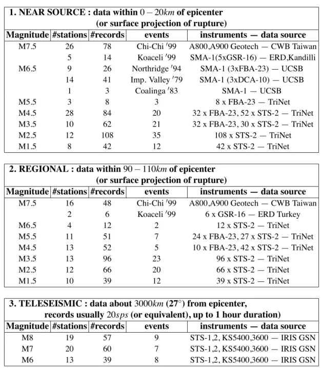
The earthquake signals selected were divided into magnitude-distance bins, summarised in Table 2.4. For each distance, the bins vary in increments of one magnitude unit, for example, the M6.5 bin incorporates data from M6.0 to M6.9 events. The three distance bins represent near-source, regional and teleseismic recordings.
The records in the near-source database were generally limited to data from within 10km distance from the projection of rupture onto the Earth’s surface. Event magnitudes
1. NEAR SOURCE : data within0−20kmof epicenter (or surface projection of rupture)
Magnitude #stations #records events instruments — data source
M7.5 26 78 Chi-Chi&99 A800,A900 Geotech — CWB Taiwan 5 14 Koaceli&99 SMA-1(5xGSR-16) — ERD,Kandilli M6.5 9 26 Northridge&94 SMA-1 (3xFBA-23) — UCSB
14 41 Imp. Valley&79 SMA-1 (3xDCA-10) — UCSB 1 3 Coalinga&83 SMA-1 — UCSB
M5.5 3 8 3 8 x FBA-23 — TriNet
M4.5 28 84 20 32 x FBA-23, 52 x STS-2 — TriNet M3.5 10 62 21 32 x FBA-23, 30 x STS-2 — TriNet M2.5 12 108 35 108 x STS-2 — TriNet
M1.5 8 42 12 42 x STS-2 — TriNet
2. REGIONAL : data within90−110kmof epicenter (or surface projection of rupture)
Magnitude #stations #records events instruments — data source
M7.5 16 48 Chi-Chi&99 A800,A900 Geotech — CWB Taiwan 2 6 Koaceli&99 6 x GSR-16 — ERD Turkey
M6.5 4 12 2 12 x STS-2 — TriNet M5.5 11 51 7 24 x FBA-23, 27 x STS-2 — TriNet M4.5 13 52 5 10 x FBA-23, 42 x STS-2 — TriNet M3.5 13 96 23 96 x STS-2 — TriNet M2.5 12 66 20 66 x STS-2 — TriNet M1.5 10 39 12 39 x STS-2 — TriNet
3. TELESEISMIC : data about3000km(27◦) from epicenter,
records usually20sps(or equivalent), up to 1 hour duration) Magnitude #stations #records events instruments — data source
M8 19 57 9 STS-1,2, KS5400,3600 — IRIS GSN M7 20 60 7 STS-1,2, KS5400,3600 — IRIS GSN M6 13 39 8 STS-1,2, KS5400,3600 — IRIS GSN Table 2.4: Summary of waveform data included in each Magnitude-Distance bin. For the teleseismic datasets — M8 is represented by events in the range M7.6 - M8.0, at 21◦- 31◦ and 33 - 480kmdepth, with 2 additional records from the M8.2 637kmdeep focus Bolivia event at 20◦— M7 is represented by events in the range M6.8 - M7.4 at 23◦- 29◦and 10 -185kmdepth — M6 is represented by events all of M6 at 25◦- 29◦and 10 - 49kmdepth.
TriNet) (www.trinet.org; www.scecdc.scec.org/stp.html) (Hauksson et al., 2001). Due to a sparsity of data from events of M6 and above, the distance limit was relaxed to include records under 20kmfrom the projection of rupture. For these larger events, data is also included from the Southern California Earthquake Center (SCEC) Strong Motion Data Base (SMDB) (now part of COSMOS,http://db.cosmos-eq.org/) for historic events, with records from predominantly analogue instruments, and from Taiwanese (Lee et al., 1999; Uzarski and Arnold, 2001) and Turkish (www.koeri.boun.edu.tr;www.deprem. gov.tr; Youd et al, 2000) data centers for timeseries from recent large earthquakes outside of Southern California.
The regional database was represented by records at a distance of about 100km. Event magnitudes range from M7.5 down to M1.5. As with the near-source database, the distance bin was relaxed to include records within 85−110kmof the projection of rupture onto the Earth’s surface for the sparse data sets from the larger magnitude events. The data sources were the same as those for the near-source database.
Records in the teleseismic database were limited to signals recorded at about 3000km epicentral distance. Data from M8 to M6 events were used, obtained from the IRIS-GSN Web site (www.iris.washington.edu).
Each bin contained records from a wide sampling of events and stations in order to obtain reasonable median values of peak amplitude. The only event which contained data which seriously deviated from the median was the M8.2 deep focus Bolivia event, which is treated separately.
All timeseries from broadband velocity instruments were differentiated to acceleration.
2.5.2
Recovery of Earth Signals
Once the database was assembled, each individual timeseries was passed through octave-wide bandpass filters. The absolute maxima of each bandpass for each record was recorded, as illustrated for 2 very different signals in Figure 2.7 and Figure 2.8. The maximum fre-quency for the bandpasses for each magnitude-distance bin was determined by the Nyquist
value of the timeseries. The minimum frequency was more subjectively chosen as the frequency where the signal intensity was similar to the background noise.
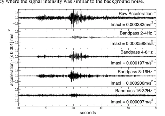
seconds acceleration - [x 0.001] m/s 2 Raw Acceleration Bandpass 2-4Hz Bandpass 4-8Hz Bandpass 8-16Hz Bandpass 16-32Hz |max| = 0.0000588m/s2 |max| = 0.000382m/s2 |max| = 0.000197m/s2 |max| = 0.000206m/s2 |max| = 0.000097m/s2
Figure 2.7: Sample bandpasses for M3.5 at 100km(acceleration records from 3 February 1998 event, recorded at Station LKL on the 80spsN-S component channel of an STS-2.
For each bandpass of a magnitude-distance bin, the geometric mean of all the absolute maxima was calculated. When combined with the geometric means from the other band-passes in the same bin, a curve is obtained which represents the octave-wide frequency content typical of ground motions for that bin. This is demonstrated for the M3.5 at 100km magnitude-distance bin in Figure 2.9.
The frequency-amplitude curves for all the magnitude-distance bins are shown in Fig-ure 2.1. In this FigFig-ure, also shown are the dynamic range performances of the instruments typically installed at a CISN station. Figure 2.10 includes the hypothetical low-gain veloc-ity meter.
The limits of the individual instruments to the broadband signals have been discussed (see Figure 2.6). The ground motion data plotted has been bandpass filtered, and to account for this, there is a need to modify, or calibrate, the broadband instrument clip levels for an octave-wide clip level. To do this, first a number of broadband timeseries are chosen which are close to clipping each instrument (generally within 20% of saturation). These records
|max| = 5.20m/s2 Raw Acceleration Bandpass 0.125-0.25Hz |max| = 0.836m/s2 Bandpass 0.25-0.5Hz |max| = 1.23m/s2 Bandpass 0.5-1Hz |max| = 0.927m/s2 acceleration - m/s 2 seconds |max| = 0.597m/s Bandpass 1-2Hz 2
Figure 2.8: Sample bandpasses for M7.5 at 10km(acceleration records from 21 September 1999 Chi-Chi earthquake, recorded at Station T076 on the 200spsZ component channel of a Geotech A900).
are then filtered in octave-wide bandpasses. To calibrate the instruments, the bandpass with the highest velocity (for the broadband STS-2 seismometer) or acceleration (for the FBA-23) is selected, this maximum value is scaled by the reciprocal of the percentage the timeseries came to the clip level for the instrument. This new value is the calibrated clip level for the bandpassed data. The inherent uncertainty in this method was reduced by performing this for a number of records of varying spectral content. Typically this reduced the broadband clipping levels by about 50% .
Finally, the New High and Low Noise Models from Peterson (1993) were superimposed onto Figures 2.1 and 2.10.
The ‘M7.5Max’ line on Figures 2.1 and 2.10 was derived from some of the largest near-source waveforms ever recorded, including data from the recent Chi-Chi, Taiwan, and Kocaeli, Turkey events. The line is constructed using the absolute maxima of each bandpass for the M7.5 at 10km dataset (not the geometric mean). From all these records, it is clear that both the±19.6m/s2 FBA-23 and hypothetical low-gain velocity instrument are unlikely to clip in the event of most conceivable Earth motions. In this regard, both
10
−110
010
110
210
−710
−610
−510
−410
−310
−210
−1High Noise Model
M3.5 at 100km
−
geometric mean
scatter points
FBA
−
23 min
Velocity Meter min
STS
−
2 clip at 13mm/s
frequency
−
Hz
octave wide bandpassed acceleration
−
m/s
2
Figure 2.9: Data scatter and geometric mean for M3.5 at 100km. The crosses are the individual data points from each timeseries (as in Figure 2.7), and their geometric mean is represented by the thick dashed-dotted line. Instrument and noise lines are similar to Figure 2.6.
10−3 10−2 10−1 100 101 102 10−11 10−10 10−9 10−8 10−7 10−6 10−5 10−4 10−3 10−2 10−1 100 101 102 High Noise Model Low Noise Model region lost region lost region gained region gained STS− 2 clip at 13mm/s STS− 2 min resolution
Velocity Meter clip at 5m/s / 5g
Velocity Meter min resolution
FBA−23 clip at 2g FBA−23 min resolution M7.5max M7.5 M6.5 M5.5 M4.5M3.5 M2.5 M1.5 M7.5 M6.5 M5.5 M4.5 M3.5 M2.5 M1.5 M8.0 (Bolivia) M7.0 M6.0 frequency − Hz
octave wide bandpassed acceleration
− m/s 2 Near Source ~ 10km Regional ~ 100km Teleseismic ~ 3000km
Figure 2.10: Frequency - amplitude plot — showing advantages of recording strong mo-tion velocity. As Fig 2.1, with on-scale momo-tions recorded by the hypothetical low-gain broadband seismometer lying between the solid blue lines. The areas shaded light blue are regions of frequency-amplitude space that are recorded by the FBA-23, but not recorded by the hypothetical low-gain broadband seismometer. Areas shaded yellow are regions of frequency-amplitude space that are recorded by the hypothetical low-gain broadband seismometer, but not recorded by the FBA-23. (see text for further explanation)
instruments would be equally effective in recording the strong motion data gathered to date.
The yellow shading in Figure 2.10 indicates regions of frequency-amplitude space that can be recorded by the hypothetical instrument, but are not presently recorded by the ac-celerometer. For the same dynamic range, the low-gain velocity instrument would record a larger range of Earth signals at periods greater than 1Hz than the accelerometer. The potential of this hypothetical device for measuring long-period motions from basin am-plifications of small, local earthquakes is obvious. Teleseismic energy at longer periods, as well as energy from smaller events at teleseismic distances, would also be recorded. Regions of frequency-amplitude space presently recorded by the accelerometer, but not recorded by the hypothetical instrument, are indicated by the blue shading in Figure 2.10.
Note that the lines of geometric mean are not representative for some large, deep tele-seismic events. The teletele-seismic database includes the M8.2 9 June 1994 637km deep fo-cus Bolivia event, and the median line for data from this event alone is also plotted on Figure 2.10. Records from this earthquake contain interesting high frequency energy not present at teleseismic distances during shallower events.
2.5.3
Recovery of Acceleration
High frequency acceleration signals derived from a single differentiation of an STS-2 veloc-ity timeseries are examined to demonstrate the likelihood of good recovery of acceleration data from the hypothetical instrument. Figure 2.11 presents a comparison of acceleration records from an STS-2 and an FBA-23. The record in question, from a M4.5 Northridge aftershock on 27 January 1994, recorded by the nearby SCSN station at Calabasas (CALB), had a recorded peak velocity (STS-2) of 1.24cm/s, within 95% of clipping the instrument. There is a close correlation of these signals, even near the clipping limit of the STS-2. A similar capability to recover ground acceleration from the hypothetical instrument is antic-ipated.
Figure 2.11: Comparison of acceleration records from a differentiated STS-2 (solid line) and an FBA-23 (dashed line). The records are from a M4.5 Northridge aftershock on 27 January 1994 recorded at Calabasas, CALB, N-S Component, 12km from the epicenter. Timeseries are from 80spschannels, with a low-pass filter at 20Hz.
2.6
‘Strong Motion’ Recordings at Teleseismic Distances
The global seismic network and database IRIS-GSN (www.iris.washington.edu) has 1sps accelerometer channels (mainly FBA-23’s) at many stations to record long-period data from the largest earthquakes. These events may cause motions that may over-drive the current broadband seismometers, even at teleseismic distances. Figures 2.12, 2.13 and 2.14 show an example of long-period motions recorded by this channel. The recordings are from station SNZO in New Zealand, and are from the M8.1 25 March 1998 event located near Balleny Island, at a distance of 2900km. The instruments at the station are a Geotech KS-36000-i down-hole seismometer (similar to the STS-2) and an FBA-23. This record is within 15% of clipping a ±13cm/s STS-2 — the earthquake actually clipped a Guralp CMG-3T (station SBA) and a Geotech/Teledyne KS-54000 (station VNDA) both set to about ±9mm/s and both at a distance of 1700km from the epicenter in Antarctica. It is clear from the records that the FBA-23 is capable of recording the event well out to periods up to about 50 seconds. This clearly shows the usefulness of the strong motion instrumentFigure 2.12: Velocity time series of 1sps integrated FBA-23 (dashed line - high-pass fil-ter at 300s) and the 20sps KS-36000-i (solid line - decimated to 1sps) recording of the Z-component of the M8.1 Balleny Island earthquake from IRIS-GSN Station SNZO at 2900km.
Figure 2.13: As Figure 2.12, but with a bandpass from 37.5 to 75 seconds, clearly showing the FBA-23 recording (dashed line) is capable of recovering long-period motion up to 50 seconds.
Figure 2.14: As Figure 2.12, but with a bandpass from 75 to 150 seconds, showing the FBA-23 recording (dashed line) is not easily resolved above the instrument noise at these amplifications.
at the IRIS-GSN stations, especially in the event of a great M9 earthquake, which could clip the high-gain broadband instruments for great distances. A low-gain velocity recording device would be ideally suited to deployment in future IRIS-GSN stations, as well as in the proposed Advanced National Seismic System.
2.7
Summary
Although the existing strong motion accelerometers generally perform well, several unde-sirable features of their response could be remedied by utilizing a strong motion sensor with a better long-period response.
Two main issues are addressed. The first issue is that records from accelerographs must be integrated twice to recover ground displacement. This double integration is an unstable procedure. In order to achieve reasonable displacements we often need to apply numerous adhoc assumptions. The second issue is that the accelerations from long-period signals (periods longer than 10 seconds) are very small. Even with 140dBof dynamic range, the signal-to-noise ratio of accelerometer records is poor for distant earthquakes. Potentially
valuable basin effects from small local earthquakes are also not recorded by the current accelerometers.
It is shown that both these problems would be alleviated by employing the hypothetical strong motion velocity instrument described here. This instrument would better utilize the large dynamic ranges — currently up to 7 orders of magnitude — available to the instrument designer by virtue of modern 24-bit digitisers.
The seismological community would benefit from this richer range of recorded motion, as many current networks built and maintained (in mostly urban areas) by the earthquake engineering community include only strong motion accelerometers. With the deployment of an instrument of the type discussed here, a station would record increased long-period data from near-source events of small magnitudes, medium-sized regional events and larger teleseisms. Continuous telemetry from a dense network of these strong motion stations would also aid development and the eventual reliability of a future real-time earthquake early warning system.
Using the proposed instrument, the engineering community would have access to re-liable estimates of near-source ground displacements without compromising the quality of acceleration records. Improved measurements of the near-source displacement records would be of important use for the development of future structural design codes, though as will be illustrated in subsequent Chapters, permanent displacements are as difficult to recover with this instruments as they are from accelerometers. Further, the strong motion velocity meter is equally sensitive to tilt as any other inertial sensor.
A strong motion velocity seismometer would essentially be a low-gain version of exist-ing broadband seismometers, such as the Weilandt-Streckeisen STS-2. Thus its cost would also be similar to other broadband seismometers, which at current prices is many times more than current 140dBaccelerometers. Unfortunately, so would its size and weight. Thus the clear advantages are likely to be offset by significantly greater cost, size and weight than an accelerometer, which would make it unwieldy for dense building instrumentation.