1 Introduction
Quantitative Precipitation Nowcasting (QPN) is one of the main applications of radar observations. On one hand, one of the most used nowcasting algorithms is Lagrangian extrapolation. It shows skill in specifying the timing and location of precipitation over short time periods, but shows low skill when using past precipitation trends to predict changes in precipitation intensity. On the other hand, Numerical Weather Prediction (NWP) models have roof skill at predicting the precise timing and location of precipitation, although they provide useful information about the intensity trends. It is therefore to investigate whether this additional information provided by NWP could be used to improve QPN.
SBMcast (Berenguer et al., 2011) is an ensemble nowcasting algorithm based on Lagrangian extrapolation of recent radar observations. It generates a set of future rainfall scenarios (ensemble members) compatible with observations and preserving the spatial and temporal structure of the rainfall field according to the String of Beads model (Pegram and Clothier, 2001). This study shows the first results obtained with a methodology to constrain the spread of SBMcast ensembles with the additional information provided by NWP.
2 Data used
Here we use observations collected with the Creu del Vent (CDV) C-band radar of the Meteorological Service of Catalonia, SMC, (Figure 1). The raw data have been processed to eliminate the ground clutter and mitigate the effect of beam blockage, thereby only considering rainfall echoes. Rainfall calibration is monitored by comparison with the observations of the raingauge network available in Catalonia (Spain). The fields used here are the surface reflectivity estimates with a spatial resolution of 1 km.
The NWP forecasts used in this study are those produced with the High Resolution Limited Area Mode (HIRLAM). This model generates 48-hour ahead hourly rainfall field forecasts, with a grid resolution of 8km.
In this study, two case studies have been analyzed to apply the proposed methodology. The first one corresponds to a stratiform situation occurred on 15 May 2013 from 10:00 to 21:00 UTC. The second case corresponds to a convective/stratiform situation on 07 Septembre 2013 at 09:00 to 15:00 UTC. This event is composed of two distinct parts, the first is clearly convective, and it evolved to a stratiform rainfall event towards the end of the period.
160 x 160 km2 Creu del Vent
(CDV)
Barcelona
(BAR)
The use of NWP forecasts to improve an ensemble
nowcasting technique
Alejandro Buil, Marc Berenguer, Daniel Sempere-Torres.
Centre de Recerca Aplicada en Hidrometeorologia, Universitat Politècnica de Catalunya,
3 The ensemble nowcasting technique SBMcast
The main objective of SBMcast (Berenguer et al., 2011) is the characterization of the uncertainty associated with the errors that affect the deterministic forecasts obtained by Lagrangian extrapolation. The main sources of uncertainty that affect these forecasts are the following (Germann et al, 2006 and Bowler et al., 2006):
1. errors due to the growth and dissipation of the precipitation intensity that are not explained by the advection of the precipitation field, and
2. errors induced by the motion field used when performing the extrapolation. On one hand, it uses a single motion field throughout the whole forecast when is known that the motion field changes in time. On the other hand, the estimation of these fields are not perfect.
The relative importance of these two uncertainty sources depends mainly on the type of event. In cases of stratiform precipitation (where its propagation is systematic and persistent) the growth and decay is well characterized by the rainfall field’s advection. Therefore, in those cases the motion field’s errors are the ones affecting most. However, in convective cases the opposite is true. But according to Germann et al.. (2006) the overall error is the growth and decay. For this reason, SBMcast is mainly focused on to characterize this predominant source of uncertainty.
SBMcast is based on the assumptions of the statistical model String of Beads Model (Pegram and Clothier, 2001) in the terms of the rainfall field’s temporal and spatial structure. This technique is extended by using a probabilistic point of view through the use of ensembles with the final goal of preserving the characteristics of the last observation.
To generate a forecast with SBMcast the following steps are performed:
1. Computation of the two global variables, Image Mean Flux (IMF), i.e. the average rainfall rate in mm/h, and Wet Area Ratio (WAR), i.e. the proportion of the domain where a rainfall rate exceeds a threshold of 1 mm/h. Clothier and Pegram (2001) showed how the IMF and the WAR are directly related to the precipitation’s mean (µ) and standard deviation (σ), respectively, of a truncated Gaussian distribution.
2. Simulation in time of IMF and WAR using an order 5 autoregressive model AR(5). Thus, the characterization of the growth and decay related with the uncertainty is ensured through the relation of IMF and WAR with the precipitation’s µ(t) and σ(t).
3. Modeling the evolution of the rainfall fields with a second order autoregressive model:
€
X
t*(
t
+
n
⋅ Δ
t
)
=
φ
1(
t
)
⋅
X
t *(
t
+
[
n
−
1]
⋅ Δ
t
)
+
φ
2(
t
)
⋅
X
t *(
t
+
[
n
−
2]
⋅ Δ
t
)
+
γ
(
t
+
n
⋅ Δ
t
)
( 3.1 ) where€
X
(
t
+
n
⋅ Δ
t
)
is the standardized rainfall field,€
φ
1(
t
)
and€
φ2(t) are the Yule-Walker coefficients and
€
γ(t+n⋅ Δt) is the noise term with
€
E[γ(t+n⋅ Δt)]=0. The latter is correlated in space according to a power –law
spectrum with exponent . The variance of
€ γ(t+n⋅ Δt) is: € Var[γ(t+nΔt)]=[1+ϕ2(t)][1+ϕ1(t)−ϕ2(t)][1−ϕ1(t)−ϕ2(t)] [1−ϕ2(t)] ( 3.2 ) 4. Imposing in Lagrangian coordinates the values of
€
IMF
(
t
+
n
⋅ Δ
t
)
and€
WAR
(
t
+
n
⋅ Δ
t
)
(described in point 1) to the fields obtained in point 2 (see further detail in Pegram and Clothier, 2001).4 Methodology
The goal of this work is to incorporate the additional information about the temporal evolution of the precipitation provided by the NWP model into the forecast algorithm SBMcast. This new source of information has been used to improve the forecast of the global variables IMF and WAR. For this purpose, the Ensemble Kalman Filter algorithm has been used, which allows the combination of the variables simulated with the NWP model, with those obtained by the radar observations.
4.1 Ensemble Kalman Filter
The Kalman filter provides a rigorous solution to the estimation of the k-th state xk through noisy measurements of y1….yk
in the case of linear systems. The Ensemble Kalman Filter (EnKf) was proposed by Evensen (1994) as an alternative to the solving of non-linear systems traditionally solved with the extended Kalman Filter. EnKF is a sequential data assimilation method, using Monte Carlo or ensemble integrations (Burgers et al.,1998). In weather forecasting this method is used in the data assimilation system, where the model and observations operators are usually non-linear, the initial states are highly uncertain, and there are a large number of measurement.
The system can be presented with a discrete-time nonlinear system with dynamics,
€
x
f k=
f
(
x
f k−1,
u
k−1)
+
w
k−1 ( 4.1 ) and measurements,€
y
k=
h
(
x
k)
+
v
k ( 4.2 ) where€
f
(
x
fk−1
,u
k−1)
is the state transition model,€
h(x
k)
is the observation model and€
v
k≈
N(0,
R
k)
and€
w
k≈
N
(0,
Q
k)
are stationary zero-mean white noise processes with covariance matrixR
k andQ
k,
respectively. The function€
f
(
x
fk−1
,
u
k−1)
explains how the state xk evolves between successive time steps and€
w
k is added to describe the model uncertainties. The observation model€
h(x
k)
defines how the state xk is related with the measurement yk. The randomvector
€
v
k represents the measurement noise, which relates to the uncertainty of the measurement yk..The next step consists basically in representing the statistical error in the forecast step. It is assumed that at time step k, it has the ensemble of q forecasts values,
€
x
k f=
(
x
k f1,...,
x
k fq)
with the mean€
x
k f. Now is possible to obtain the ensemble error matrix, in the forecast step (
€
E
k f) and the measurements (
€
E
ykf) around the ensemble mean because the state xk is unknown.
Thus is considered the forecast ensemble mean as the best forecast estimate of the state xk.
With this, we can obtain the covariance matrices of the error associated with the measurements and the forecast
€
P
k f=
1
q
−
1
E
k f(
E
k f)
T ,€
P
xyk f=
1
q
−
1
E
k f(E
yk f)
T ,€
P
yyk f=
1
q
−
1
E
yk f(
E
yk f)
T ( 4.3 )The second step is the analysis steps. To obtain the final state the next equation is applied
€
x
kai=
x
kfi+
K
k(
y
ki−
h(x
kfi))
( 4.4 ) where€
K
kis the Kalman gain which provides the weight given to the observation with respect to the forecast step. It is defined by€
K
k=
P
xyk f(
P
yyk f)
−1 and€
y
ki are the perturbed observations. Once we obtain€
x
kai, 4.1 is applied iteratively.4.2 Application of the ensemble Kaman filter algorithm
The Ensemble Kalman Filter formalism described above has been applied with the goal of improving the forecasts of the SBMcast global variables IMF and WAR. The goal is to incorporate the rainfall field information that NWP models can provide. Such models are interesting, because they are capable of generating forecasts for periods of time much longer than those obtained through the extrapolation of the radar rainfall fields.
In this work the state variable xk, which we attempt to forecast is defined as the bivariate variable
€
x
k=
IMF
R *WAR
R*⎛
⎝
⎜
⎞
⎠
⎟
( 4.5 )where IMFR* y el WARR* are the two normalized global variables obtained from radar observations (R) of the rainfall field.
The noisy measurements yk are defined as:
€
y
k=
IMF
M *WAR
M *⎛
⎝
⎜
⎞
⎠
⎟
( 4.6 )where the IMFM* and WARM* have been obtained from forecasts obtained from the NWP model (M). The covariance
matrices
R
k andQ
k and the transition model€
f
(
x
fk−1
,
u
k−1)
were obtained through the long-term analysis of the eventsthroughout the year 2013 and the first part of 2014. Since we work with normalized variables, the observation model corresponds to the identity matrix:
h(
x
k)
=
1 0
0 1
⎛
⎝
⎜
⎞
⎠
⎟
(x
k)
( 4.7 )5 Results
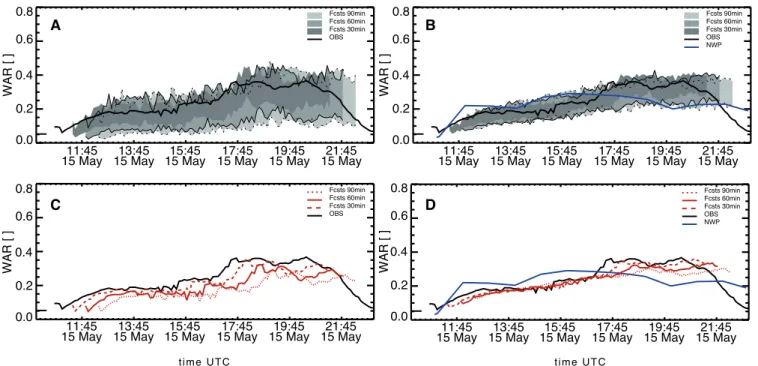
The quality of the forecasts realized by SBMcast largely depends on its capacity to correctly estimate the global variables IMF and WAR. Figure 2 shows an example of the evolution of the simulated and observed WAR, for the event of 15 May 2013. In Figures 2a and 2b the comparison between the observations (black line) and the probabilistic forecasts using the AR(5) model and the EnKf, respectively, are displayed. For this purpose we only show the values between the 10%-90% percentiles corresponding to the 30, 60, and 90 minute-ahead forecasts. In both cases the confidence interval covers the observed WAR values most of the time. However, the spread obtained with the AR(5) model is much larger than in the EnKf case.
In Figures 2c and 2d the deterministic component of both previously mentioned forecasts is shown. It can be seen that with the AR(5) model underestimate the observed WAR. It is most visible for the 90 minute ahead forecast. In the case of the forecast using EnKf it can be seen that mainly in the central part of the episode the deterministic forecast is almost perfect independently of the lead time of the forecast. Towards the end of the episode, the NWP starts being more imprecise. For this reasons the forecasts are more similar to the ones provided by the AR(5) mode.
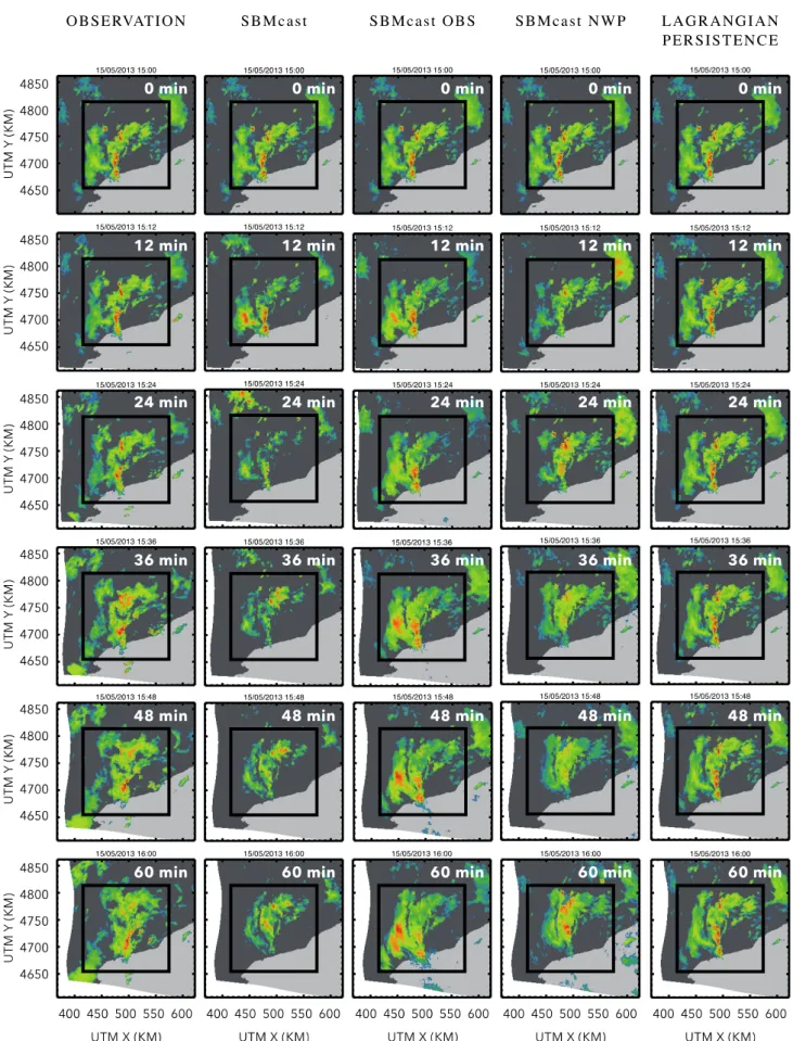
Figure 3 shows an example of the rainfall field forecasted for lead times up to 1h with the different SBMcast versions. These versions correspond to different ways to estimate the IMF and WAR. In SBMcast OBS and SBMcast NWP we have directly imposed the observations and the simulation of the EnKf, respectively. The right column displays the results of the deterministic algorithm Lagrangian Persistence. In the center columns a member of the ensemble with the different configurations of the SBMcast is depicted, this fact can be compared with the observations in the left column. It can be seen that while with the Lagrangian persistence the intensity remains constant along the forecasts, the members of the probabilistic nowcasting evolve in time.
Figure 2: Evolution of the WAR during the event of 15 May 2013. In all panels, the solid black line corresponds to the values computed with the observations. The shaded areas correspond to the ensemble of simulated values (50 members) between the 10% and 90% percentiles for the 30,60,90 minutes ahead predictions. a) Results obtained with the AR(5) model originally used in SBMcast, b) results obtained with the EnKf, c) deterministic component of the WAR forecasted with an AR(5) model, and d) Deterministic component of the
WAR forecasted with the EnKf.
11:45
15 May 15 May13:45 15 May15:45 15 May17:45 15 May19:45 15 May21:45 0.0 0.2 0.4 0.6 0.8 WAR [ ] OBS Fcsts 30min Fcsts 60min Fcsts 90min NWP OBS Fcsts 30min Fcsts 60min Fcsts 90min 11:45
15 May 15 May13:45 15 May15:45 15 May17:45 15 May19:45 15 May21:45 0.0 0.2 0.4 0.6 0.8 WAR [ ] OBS Fcsts 30min Fcsts 60min Fcsts 90min 11:45
15 May 15 May13:45 15 May15:45 15 May17:45 15 May19:45 15 May21:45 0.0 0.2 0.4 0.6 0.8 WAR [ ] NWP OBS Fcsts 30min Fcsts 60min Fcsts 90min 11:45
15 May 15 May13:45 15 May15:45 15 May17:45 15 May19:45 15 May21:45 0.0 0.2 0.4 0.6 0.8 WAR [ ] A
time UTC time UTC
B
Figure 3:Evolution of the precipitation field as forecasted with the tested nowcasting techniques for the event of 15/05/2013 at 15:00 UTC. From left to right: observed reflectivity fields, one member of the different configurations of SBMcast, deterministic forecast by
The performance of the probabilistic forecast quality has been assessed by means of two probabilistic skill scores widely used in the literature. They are defined as a function of the lead time.
(1) The Conditional Square Root of Ranked probability (CSRR) is defined as:
€ CSRR(τ)= 1 Ωt 0+τ(max−min) [P(t0+τ,x,)−Pʹ′(t0+τ,x,)]2ddx min max
∫
Ω∫
⎧ ⎨ ⎪ ⎩ ⎪ ⎫ ⎬ ⎪ ⎭ ⎪ 2 ( 5.1 ) where€
Ω
t0+τis the size of the observed precipitation domain,€
P
(
t
0+
τ
,
x
,)
is the probabilistic forecast and€
Pʹ′(t
0+
τ
,
x,
)
is the observation for each threshold€
. For perfect forecast the CSRR is zero. (2) Brier Score is defined as:€
Brier
(τ
)
=
1
n
x∑
,y,t[
f
t(
x
,
y
,
t
+
τ)
−
p
(
x
,
y
,
t
+
τ
)]
2 ( 5.2 ) where€
p(x,
y,t
+
τ)
is the observed probability and€
f
t(
x
,
y
,
t
+
τ
)
is the forecast probability at time t for alocation (x,y) and with a lead time
€
τ
. It has been obtained for a threshold of 1 mm/h. For perfect forecast the Brier score is 0.With the aim of performing a more exhaustive analysis of the results, the previous results are compared with two other nowcasting algorithms: (i) the deterministic version of Lagrangian extrapolation, and (ii) the local Lagrangian probabilistic algorithm; it generates forecasts for the probability distribution of a given point in the field, examining the spatial variability of the precipitation field, in Lagrangian coordinates. Germann and Zawadzki (2004) compared four different probabilistic methods and found that this method to have the best performance.
In the comparison of Figure 4, we have also included a modified version of SBMcast (SBMcast-OBS). In this, we have directly imposed the observations of IMF and WAR a posteriori. This allows us to quantify the impact of using the best possible forecasts of the global variables IMF and WAR, Therefore, it is possible to detect the best possible result by only modifying this part of the algorithm.
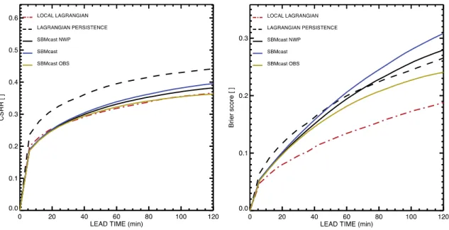
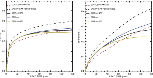
Figures 4 and 5 show the skill scores for the two considered events. We can observe that, for the 40-50 minute ahead and longer-term forecasts, the inclusion of the additional information of the NWP model to SBMcast (SBMcast-NWP) improves the results compared with the original SMBcast configuration. In the case stratiform rainfall (15 May 2013) it can be seen that the Local Lagrangian behaves similarly as SBMcast-OBS for all rainfall thresholds (CSRR). However, in terms of the Brier Score obtained for the same event, the Local Lagrangian clearly performs better. In the event of the 07 September 2013, partially convective, it can be seen that for lead times larger than 60 minutes SBMcast-OBS obtains a better performance than the Local Lagrangian. Looking closely at the CSRR and Brier score figures, it can be seen that the SBMcast-NWP curve falls between the original SBMcast and SBMcast-OBS curves for both cases.
Figure 5: Average CSRR (left) and Brier score (right) for the event of 7 September 2013 for the different nowcasting algorithms.
6 Conclusions
The contribution of this work lies in the improvement of the SBMcast algorithm by adapting it to the inclusion of external data with the aim of improving the state of the art forecasts. For this purpose we have used rainfall fields generated with the NWP model HIRLAM. The proposed algorithm to integrate these data is the Ensemble Kalman Filter.
The results show that the integration of the additional information to simulate the global variables IMF and WAR helps improving the rainfall field forecasts. Only in the shorter term forecasts the proposed method (SBMcast-NWP) behaves similarly to the original SBMcast; while for lead times beyond 30 minutes it clearly shows a better performance. The small difference in performance for shorter term forecasts is due to the fact that the additional NWP information does not provide a significant contribution with respect to the past observations. At around 30 minute ahead forecast the additional information becomes valuable. In the case of the simulations obtained with the Ensemble Kalman Filter the forecasts have a smaller spread compared with the observations obtained with the AR(5) for the considered events.
Moreover, as the CSRR figures show, the exact forecast of the IMF and the WAR allows for an improvement in the forecasts, leading to results comparable with those of the Local Lagrangian, an outperforming this method in the case of convective events. The performance of the deterministic forecasts in both events is worse than the performance of the probabilistic algorithms. This difference is more marked in the convective events where the rainfall growth and decay is the major source of error.
Finally, it is worth mentioning that, in general, the best results are obtained with the Local Lagrangan algorithm. This allows benefits from larger sampling sizes to generate the probabilistic nowcasts as the lead time increases. The result is smoother probabilistic nowcasts that minimize the errors in the pdfs. In comparison, the main advantage of SBMcast nowcasts is that they respect the space and time structure of the precipitation fields.
Acknowledgements
This work has been carried out in the framework of the project ProFEWS (CGL2010-15892) funded by the Spanish Ministry of Economy and Competitiveness (MINECO). Radar observations used in this study were provided by the Meteorological Service of Catalonia (SMC). HIRLAM forecasts were provided by the Finnish Meteorological Institute (FMI).
References
Berenguer, M., D. Sempere-Torres, and G. G. S. Pegram, 2011: SBMcast - An ensemble nowcasting technique to assess the uncertainty in rainfall forecasts by Lagrangian extrapolation. Journal of Hydrology, 404, 226-240.
Bowler, N. E., C. E. Pierce, and A. W. Seed, 2006: STEPS: A probabilistic precipitation forecasting scheme which merges an extrapolation nowcast with downscaled NWP. Quarterly Journal of the Royal Meteorological Society, 132, 2127-2155. Burgers, G., P. Jan van Leeuwen, and G. Evensen, 1998: Analysis Scheme in the Ensemble Kalman Filter. Monthly
Clothier, A. N., and G. G. S. Pegram, 2001: Space-time modelling of rainfall using the String of Beads mode: Integration of radar and rain gauge data. W. R. Commission, Pretoria, South Africa.
Evensen, G., 1997: Advanced Data Assimilation for Strongly Nonlinear Dynamics. Monthly Weather Review, 125, 1342-1354.
Germann, U., and I. Zawadzki, 2004: Scale Dependence of the Predictability of Precipitation from Continental Radar Images. Part II: Probability Forecasts. Journal of Applied Meteorology, 43, 74-89.
Germann, U., I. Zawadzki, and B. Turner, 2006: Predictability of Precipitation from Continental Radar Images. Part IV: Limits to Prediction. Journal of the Atmospheric Sciences, 63, 2092-2108.
Pegram, G. G. S., and A. N. Clothier, 2001: High resolution space-time modelling of rainfall: the "String of Beads" model. Journal of Hydrology, 241, 26-41.