PREDICTIVE ANALYTICS FOR ELECTRICITY PRICES USING FEED-INS FROM RENEWABLES. Complete Research

Complete Research

Feuerriegel, Stefan, University of Freiburg, Platz der alten Synagoge, 79098 Freiburg, Germany, [email protected]

Riedlinger, Simon, University of Freiburg, Platz der alten Synagoge, 79098 Freiburg, Germany, [email protected]

Neumann, Dirk, University of Freiburg, Platz der alten Synagoge, 79098 Freiburg, Germany, [email protected]

Abstract

Since the liberalization of European electricity markets, stakeholders can actively participate in the trading of electricity. Successful participation in such markets requires an accurate forecast of future electricity prices. However, as large volumes of energy from renewable sources are fed into the system, electricity prices are highly volatile. While recent approaches put a strong focus on models from time series analysis using merely historic prices, only a few study the influence of exogenous predictors. This paper includes both expected solar power generation and expected wind power generation as exogenous predictors and improves state of the art by assessing their beneficial impact when evaluating our forecasting models with a two-pronged approach. First, we show that these externals decrease root mean squared errors by between 3.37 % and 9.86 %. Second, we apply a Diebold-Mariano test to prove statistically that the forecasting accuracy of the models including exogenous predictors is superior.

Keywords: Business Intelligence, predictive analytics, electricity prices, forecasting accuracy, decision support, decision making/makers

1 Introduction

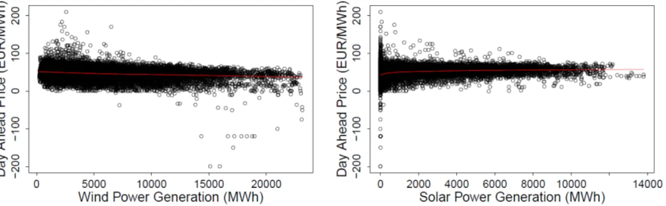
Governments around the world have triggered an energy transition from fossil fuels to renewable energies. For example, the European Union strives to have renewable sources make up 20 % of energy consumption by the year 2020. In contrast to the so-called baseload energy sources, such as coal or nuclear power, the feed-in from renewable electricity sources is highly dependent on weather conditions. Thus, the volatile nature of renewable electricity sources comes at the cost of considerable fluctuations in electricity prices (e. g. Green & Vasilakos, 2010; Woo et al., 2011). As an example, the weather dependency of German electricity prices is shown in Figure 1. These plots depict the relationship between electricity prices and expected power generation from renewables, where the trend line reveals a small but visible correlation. After having identified a discernible correlation between electricity prices and expected feed-ins, this motivates the inclusion of both variables in a model for predictive analytics.

The introduction of renewables had a dramatic effect on electricity prices, which have started to fluctuate more strongly. Nowadays, all stakeholders in electricity markets must not only devise tools to hedge price risks, but must also adapt to electricity markets, where supply does not always perfectly accommodate

Figure 1. Scatterplot of hourly day-ahead electricity prices and expected generation of wind (left) and solar (right) power with LOWESS trend line (in red) from November 1, 2009 to March 21, 2012 (EEX, 2013; EPEX, 2013).

demand. Both tasks rely heavily upon accurate price forecasts (Nogales et al., 2002). With an accurate next-day price forecast, a producer can develop an appropriate bidding strategy to maximize ones own benefit, or so a consumer can maximize its utility (Contreras et al., 2003).

The prediction analytics is a native mission ofBusiness Intelligence; it is natural to harnesses its methods

and techniques in order to derive and optimize price forecasts (Turban, 2011). Interestingly, a recent MISQ

review claims that“predictive analytics are rare in mainstream IS literature, and even when predictive

goals or statements about predictive power are made, they incorrectly use explanatory models and metrics”

(Shmueli & Koppius, 2011). In the domain of electricity price forecasts as a specific example, the existing literature (cf. Aggarwal et al., 2009; Li et al., 2005; Weron, 2006) focuses primarily on both classical time series analysis and statistical learning. These works usually ignore the predictive power of external parameters, such as weather conditions. In this setting, Business Intelligence can improve price forecasts by explicitly incorporating exogenous predictors (Shmueli & Koppius, 2011). As a result, we propose a forecasting framework that includes expected feed-ins from wind and solar power to take weather conditions into account. Here, predictive analytics is valuable for theory building and, by following this approach, this paper aims to improve the accuracy of electricity price forecasts as a contribution to Business Intelligence.

The remainder of this paper is structured as follows. Section 2 provides a literature overview of Business Intelligence publications forecasting electricity prices, where the majority of models ignores external impacts. To close this research gap, Section 3 utilizes both time series analysis and statistical learning to present models that incorporate exogenous predictors. These models are evaluated in Section 4, which, finally, reveals that external inputs improve forecasting accuracy at a statistically significant level.

2 Related Work

To fully capture the concepts of electricity price forecasting, we start by presenting different angles of the existing predictive analytics approaches. These models can be distinguished by (i) their forecasting horizon, (ii) the type of the underlying model and (iii) the externals used. Based on this literature review, we conclude this section by deriving our research question and providing evidence that the addressed research question is relevant and important to the IS community.

The different approaches to price prediction in electricity markets can be roughly classified (Cruz et al.,

price forecasts. Each time horizon is used along with a different objective. More precisely,long-termprice forecasts aim at profitability analysis and strategic planning with a horizon of at least 12 months, whereas

in themedium-term, month-ahead forecasts support risk management and derivative pricing.Short-term

forecasts cover time spans from a few hours to a few days. The latter, in particular, deserves attention:

“Since the day-ahead spot market typically consists of 24 hourly auctions that take place simultaneously one day in advance, forecasting with lead times from a few hours to a few days is of prime importance in day-to-day market operations”(Misiorek et al., 2006). To support day-to-day market operations, this paper focuses on short-term forecasts of day-ahead prices.

In addition to forecasting horizons, one can also classify price forecasting according tomethodology. In

the literature, countless forecasting strategies are proposed in order to estimate the future development of spot prices. This section does not attempt to make a thorough presentation of the known techniques, but rather provides a general classification. Existing approaches can be broadly divided into six groups

(Weron, 2006): cost-based models,game theoretic approaches,fundamental (or structural) methods,

econometric models,statistical approachesandartificial intelligence-based techniques. In particular, time series approaches (Bierbrauer et al., 2007) have been used extensively to forecast electricity spot prices. Readers interested in a detailed taxonomy should refer to a literature overview such as Aggarwal et al. (2009), Li et al. (2005) and Weron (2006).

Recently, researchers have introduced spot price models includingexogenous variables. This approach is

motivated by the assumption that price patterns are the characteristic result of underlying fundamentals

(Erni, 2012). According to Keles et al. (2013),“up to now, hardly any financial or time-series modeling

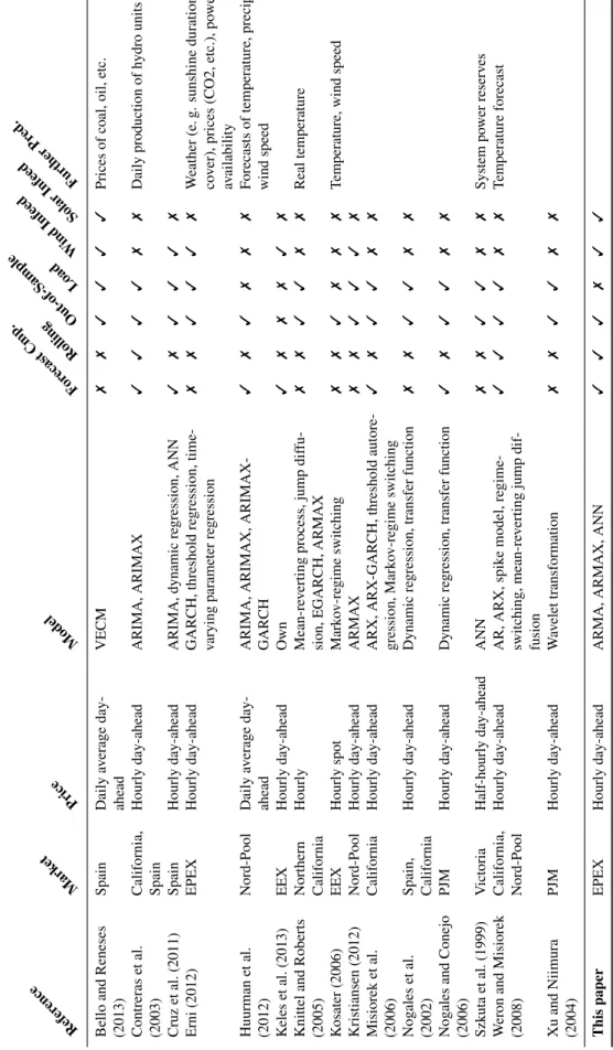
approach exists, which explicitly model the wind power feed-in and which incorporates this uncertain parameter in an integrated time-series or financial model for electricity spot prices”. In fact, we are aware of only a very few studies that actually deal with such models. All publications found are listed in the table on page 4.

When these papers are looked at in depth, we observe that most publications forecast hourly day-ahead prices. However, those works that predict average daily prices will hardly be useful for day-to-day market operations. Many references focus on grid load as an exogenous input, in contrast to only a few dealing with wind and solar power generation to model the supply side. Huurman et al. (2012) point out that most studies report in-sample errors only, and do not evaluate the out-of-sample predictive performance. Furthermore, hardly any paper analyzes to a sufficient extent how adding external parameters can result in improved accuracy. In addition, Contreras et al. (2003) as well as Weron and Misiorek (2008) measure the beneficial effect of re-estimating models for each trading day, though neglect a detailed comparison. In summary, none of the aforementioned references study the positive influences on forecasting accuracy when both wind and solar power generation are included in the model.

Hence, this paper addresses the following research question: we propose and compare models to forecast hourly day-ahead electricity prices with weather conditions considered implicitly as exogenous predictors. Thus, we outline a forecasting framework that includes expected feed-ins from both wind and solar power generation to model the supply side. In addition to that, we implement a rigorous evaluation of out-of-sample errors across a multiple year horizon. Based on this, we identify and measure the beneficial effects of incorporating these feed-ins. To allow for time-dependent parameters, we also use a moving windows of training data in order to study the rolling re-estimation of coefficients.

Refer ence Mark et Price Model For ecast Cmp. _Rolling Out-of-Sample Load W ind Infeed Solar Infeed Further Pr ed. Bello and Reneses (2013 ) Spain Daily av erage day-ahead VECM 7 7 3 3 3 3 Prices of coal, oil, etc. Contreras et al. (2003 ) California, Spain Hourly day-ahead ARIMA, ARIMAX 3 3 3 3 7 7 Daily production of h ydro units Cruz et al. (2011 ) Spain Hourly day-ahead ARIMA, dynamic re gression, ANN 3 7 3 3 3 7 Erni (2012 ) EPEX Hourly day-ahead GARCH, threshold re gression, time-v arying parameter re gression 7 7 3 3 3 7 W eather (e. g. sunshine duration, cloud co v er), prices (CO2, etc.), po wer plant av ailability Huurman et al. (2012 ) Nord-Pool Daily av erage day-ahead ARIMA, ARIMAX, ARIMAX-GARCH 3 7 3 7 7 7 F orecasts of temperature, precipitation, wind speed K eles et al. (2013 ) EEX Hourly day-ahead Own 3 7 7 7 3 7 Knittel and Roberts (2005 ) Northern California Hourly Mean-re v erting process, jump dif fu-sion, EGARCH, ARMAX 7 7 3 3 7 7 Real temperature K osater (2006 ) EEX Hourly spot Mark o v-re gime switching 7 7 3 7 7 7 T emperature, wind speed Kristiansen (2012 ) Nord-Pool Hourly day-ahead ARMAX 7 7 3 3 3 7 Misiorek et al. (2006 ) California Hourly day-ahead ARX, ARX-GARCH, threshold autore-gression, Mark o v-re gime switching 3 7 3 3 7 7 Nog ales et al. (2002 ) Spain, California Hourly day-ahead Dynamic re gression, tr ansfer function 7 7 3 3 7 7 Nog ales and Conejo (2006 ) PJM Hourly day-ahead Dynamic re gression, transfer function 3 7 3 3 7 7 Szkuta et al. (1999 ) V ictoria Half-hourly day-ahead ANN 7 7 3 3 7 7 System po wer reserv es W eron and Misiorek (2008 ) California, Nord-Pool Hourly day-ahead AR, ARX, spik e model, re gime-switching, mean-re v erting jump dif-fusion 3 3 3 3 7 7 T emperature forecast Xu and Niimura (2004 ) PJM Hourly day-ahead W av elet transformation 7 7 3 3 7 7 This paper EPEX Hourly day-ahead ARMA, ARMAX, ANN 3 3 3 7 3 3

3 Modeling Electricity Prices

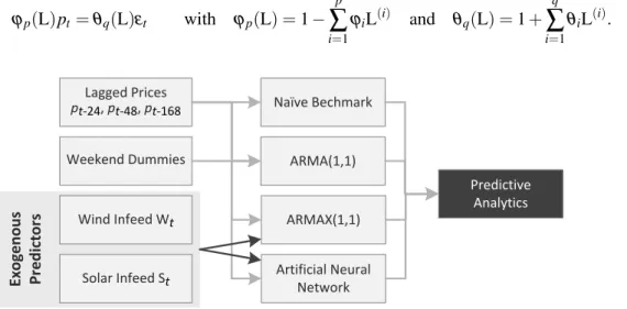
This section introduces the theoretical background on modeling electricity prices. Consistent with the existing literature, we start with a naïve approach and an ARMA model as benchmark models. We then extend classical forecasting models via exogenous predictors according to Figure 2. To gain new predictive analytics, we utilize both ARMAX models from time series analysis and Artificial Neural Networks (ANN) from statistical learning.

Let pt witht∈ {1, . . . ,N}denote the time series of electricity prices. Following Conejo et al. (2005)

and Misiorek et al. (2006), we employ a naïve but challenging test to verify that our proposed models

are better than just random guessing. According to this test, we set the forecast ˜pt topt−168, which is

the historic price from 7 days before timet. Any proposed model would pass the naïve test if its error

is smaller than the error of the naïve approach. Misiorek et al. (2006) report that in some time periods, almost all of their models have trouble passing this test. The reason why the naïve model already provides a good estimate is due to the strong repetitive pattern of intra-day and intra-week seasonality of electricity prices.

3.1 Benchmark: ARMA Model

In time series analysis, autoregressive-moving-average (ARMA) models describe a stationary stochastic process in terms of two summands: one for auto-regression and the second for the moving average. More precisely, the process is modeled as a linear combination of previous values and past errors. In that case,

both the mean and autocovariance of the series are independent of time. The notation ARMA(p,q)refers

to a model withpautoregressive terms andqmoving-average terms given by

pt=ϑ+ p

∑

∑

with suitable coefficientsϑ,ϕ1, . . .,ϕp,θ1, . . .,θqand white noise error termsε1, . . . ,εt. The coefficients

are estimated by maximum likelihood estimation (MLE). Let L denote the lag (or backshift) operator

L(h)pt=pt−h. Then, the ARMA(p,q)process can be rewritten more concisely as

ϕp(L)pt=θq(L)εt with ϕp(L) =1− p

∑

∑

When it comes to determining the ARMA orders pandq, one frequently relies on the minimization of information criterion, such as AIC (Akaike Information Criterion) or BIC (Bayesian Information Criterion).

3.2 ARMAX Model

The autoregressive-moving-average model with exogenous inputs (ARMAX) extends the classical ARMA

model by an additional linear combination of exogenous variables. Thekexogenous time series are given

byx(_t1), . . .,x_t(k). Then, the notation ARMAX(p,q)withkinputs refers to the process

pt=ϑ+ p

∑

∑

∑

with suitable coefficientsϑ, ϕ1, . . ., ϕp, θ1, . . ., θq,η1, . . ., ηk and white noise error termsε1, . . . ,εt.

Obviously, ARMAX models can be helpful tools to model electricity prices when prices are dependent not only on past values but also on exogenous inputs, such as expected wind or solar feed-ins.

3.3 Feed-Forward Artificial Neural Network

Artificial Neural Networks (ANN) are computational models inspired by the central nervous system in order to perform statistical learning (e. g. Bishop, 2009; Hastie et al., 2013). These networks are usually

represented as a system of connectedneurons, which compute values according to a mathematical function

f :X→Y from inputs by feeding information through the network. These neurons are arranged in three

(or more) layers. The first layer consists of input neurons receiving the input vectorx= [x1, . . . ,xN]T ∈X.

In our model, the input values are given by a set of historic prices and exogenous predictors. These values are then sent to a second hidden layer of neurons and, finally, to a third layer of output neurons computing

a responsey∈Y. In our case, the third layer consists of a single output neuron that predict the electricity

price. When the neurons are connected as a directed graph without cycles, this is called afeed-forward

Artificial Neural Network, which is a common neural network type in electricity price forecasting (e. g. Szkuta et al., 1999).

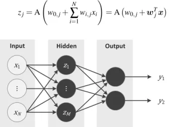
The actual calculation of f is performed as follows. The inputzjof each neuron j=1, . . . ,Mis a weighted

sum of all previous neurons calculated as

zj=A w0,j+ N

∑

Figure 3. Schematic representation of the neurons in a feed-forward Artificial Neural Network grouped into input, hidden and output layer.

wherexiare the values from the input layer and suitable coefficientswi,jfori=1, . . . ,Nand j=1, . . . ,M.

The predefined non-linear function A is referred to as theactivation function. Here, we use the logistic

function A(z) = (1+e−z)−1_.

In supervised learning, feed-forward Artificial Neural Networks are fitted to the data by learning algorithms

during a training process. For example, a back-propagation algorithm determines the parameterswi,jfor

i=1, . . . ,N and j=1, . . . ,Mby reducing the error between the true electricity price and the predicted

value from the output layer. In contrast to ordinary regressions (such as in ARMA models), feed-forward Artificial Neural Networks are a universal approximator among continuous functions under certain mild assumptions.

4 Forecasting Electricity Prices

This section evaluates mathematical models for forecasting electricity prices. After having specified the mathematical models, we now state the used datasets, including the exogenous predictors. Following this, we present the forecasting framework and give details on how to measure the forecasting accuracy. Ultimately, we verify, by comparing different models, our research question that models including wind and solar feed-ins exhibit superior accuracy.

4.1 Datasets and Descriptive Statistics

In the following evaluation, we use electricity prices from the so-calledEuropean Power Exchange(EPEX

SPOT). The EPEX operates both intraday and day-ahead markets for Germany, Austria, France and

Switzerland. These markets feature high volumes, for instance, the day-ahead trading volumes1for the

German and Austrian market combined totaled 245.3 TWh in 2012, with an increasing trend. Trading is performed continuously 7 days a week.

All prices are based on German and Austrian hourly day-ahead spot prices from January 11, 2009 to March 21, 2012 of the European Power Exchange, giving a total of 20,928 observations. This diagram indicates that prices are highly volatile. In particular, several positive and negative price spikes occur, mostly in December and January of each year. In addition, very high prices are encountered in February 2012 due

to extreme weather conditions. According to Table 2, the mean price accounts for 46.82e/MWh, with a

standard deviation of 15.76e/MWh. Electricity prices range from about −200e/MWh to 210e/MWh.

Interestingly, the kurtosis of 14.65 is substantially higher than 3, indicating the existence of heavy tails, which are probably caused by price spikes. Overall, we can deduct the following characteristics of the EPEX day-ahead prices: high volatility, negative/positive price spikes, mean reversion and strong seasonality.

1 EPEX. Volumes in 2012 on European Power Exchange EPEX SPOT hit new record. Retrieved on August 7, 2013 from http://www.epexspot.com/en/press-media/press/details/press/Volumes_in_2012_on_european_power_exchange_ EPEX_SPOT_hit_new_record.

Weekly Average Time MWh 2009−11 2010−02 2010−05 2010−08 2010−11 2011−02 2011−05 2011−08 2011−11 2012−02 0 4000 10000

Figure 4. Average weekly curves of both expected wind power generation (black) and expected solar power generation (gray) from November 11, 2009 to March 03, 2012 (EEX, 2013).

As external predictors, we utilize the following exogenous time series: the expected wind power generation and the expected solar power generation. In many countries, regulatory publication requirements obligate transmission operators to release these expected volumes day-ahead. In Germany, this happens online via EEX (2013). In addition to the expected volumes, the platform also publishes the real values afterwards. Both time series, expected and real values, are highly correlated (Erni, 2012). However, to account for a correct chronology, we rely upon the expected volumes as exogenous parameters, which are reported one day in advance. Figure 4 visualizes the average weekly expected power generation, showing both the seasonal patterns of solar power and the frequent fluctuations in wind power. With a closer look at the forecasted volumes (see Table 2), we observe the following patterns: hourly expected wind infeeds range from about 0 MWh to 23,100 MWh, with a mean of 5027 MWh. Hourly expected solar infeeds range from 0 MWh to 13,800 MWh, with a mean of 1330 MWh. Both distributions are highly volatile and positively skewed, which indicates that wind generation and solar generation are often relatively low.

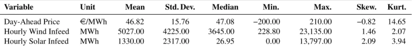
Variable Unit Mean Std. Dev. Median Min. Max. Skew. Kurt.

Day-Ahead Price e/MWh 46.82 15.76 47.08 −200.00 210.00 −0.82 14.65

Hourly Wind Infeed MWh 5027.00 4225.00 3645.00 228.80 23,135.00 1.46 2.07

Hourly Solar Infeed MWh 1330.00 2317.00 26.95 0.00 13,797.00 2.09 3.94

Table 2. Descriptive statistics of day-ahead electricity prices and exogenous predictors.

4.2 Forecasting Framework

This section presents the forecasting framework to predict electricity prices. Since our target is to compare

the above models in terms of their forecasting accuracy, we need to calculate theout-of-sampleerror. In

other words, instead of measuring the model fit by using historic data, we need to estimate the model

parameters withtrainingdata and, subsequently, evaluate our models using differenttestingdata. As

Section 4.1 shows no evidence of annual seasonality, we choose and compare two different training sets of 21 days (504 hours) and 7 days (168 hours) respectively.

To outline the time framework, Figure 5 sketches the general chronology of events. The EPEX auction design requires participants to place bids for all delivery periods day-ahead, therefore, our forecasting framework needs to make 24-hour-step forecasts. To exploit these forecasts, all predictions must be available no later than 12 a. m., which is the time when the EPEX order book closes. For the calculation, we also need the values of our exogenous predictors. This is straightforward when it comes to seasonal dummies and historic prices, however, expected feed-ins from solar and wind power generation are published – after the order book closes – at 6 p. m.. While this problem could be solved by changing the regulatory publication requirements in the future, other solutions are at hand. One could instead inject

alternative infeed predictions, modeled according to weather conditions. As recent references (e. g. Keles et al., 2013) prove, this is an active research topic and a viable alternative. Numerous authors, such Erni (2012), Keles et al. (2013) and Knittel and Roberts (2005), neglect the correct timings and rely upon the expected feed-ins. Consequently, we follow the same approach. Future versions of this research paper will also compare models with feed-ins that have been perturbed by a random disturbance term in order to further improve the validity of the model comparison.

When estimating the parameters of our models, we can choose between two options: (i) coefficients can either be determined once based on a training set, and, then, remain fixed throughout the whole testing set. Alternatively, (ii) coefficients can be re-estimated daily for each forecast using a moving window of training data. Each re-estimation takes a new training set into account, shifted by one day. This idea is

referred to as arolling re-estimationof parameters. Though increasing computational needs, one can claim

that this approach improves accuracy since the model is updated, based on new price information. Figure 6 compares both approaches graphically, where the upper part presents the notion of fixed parameters and the bottom schedule shows how parameters are re-estimated based on a shifted training set. As noted in Section 2, related publications adopt the concept of re-estimating model parameters for every forecast only rarely. Hence, we implement both options – singular parameter estimation, as well as rolling re-estimation – and compare their performances.

4.3 Forecasting Accuracy

To assess the predictive power of the proposed models, we utilize different statistical metrics to measure

the forecasting accuracy. Let ˜pt witht∈ {1, . . . ,N}denote the predicted time series. We can then check

the out-of-sample forecasting accuracy afterwards, once the true market prices pt are available. For

the time horizon under study, we calculate the following common prediction errors, namely, the Mean Absolute Error (MAE) and the Root Mean Squared Error (RMSE) given by

MAE= 1 N N

∑

∑

These are typically used in the literature on electricity price forecasting (see e. g. Conejo et al., 2005; Keles et al., 2013; Misiorek et al., 2006).

4.4 Estimating Models

In order to be able to estimate an ARMAX process, we need to check that the underlying time series is stationary. Thus, a common approach is to apply the augmented Dickey-Fuller (ADF) test, where the

t Forecasted Period of Day d+1 Trading Day d Market Clearing at 12 am Infeed Forecasts at 6 pm Electricity Delivery

Fixed Training Set Test 1 Test 2 Test 3

Training Set 1 Test 1

Training Set 2 Test 2

Training Set 3 Test 3

d=0 d=T d=T+1 d=T+2 d=T+3

Rolling Re-Estimation

Fixed Parameters

Figure 6. Comparison of fixed parameters (top) and rolling re-estimation of parameters with a moving window of training data (bottom).

null hypothesis assumes that the series under study is not stationary. In this instance, we use the training period from January 11, 2010 to January 31, 2010 as input to the ADF test. The test statistic returns −6.752 for hourly day-ahead electricity prices, −4.212 for expected wind power generation and −7.998

for expected solar power generation – all withP-values smaller than 0.01. As a result, the null hypothesis

of non-stationarity for all three series can be rejected at any given significance level. Since, the time series

is stationary, transformations, such as differentiating, are not necessary, and we can use an ARMAX(p,q)

process.

After checking stationarity, we need to choose the model parameters, i. e. the numberpof auto-regressive

and the numberqof moving-average terms. While varying the parameters pandq, we compare models

in terms of the Akaike Information Criterion corrected for finite samples. Based on this, we select an

ARMAX(1,1) process. To check if the model is able to catch all non-random effects, we study the

distribution of the standardized residuals. Less than 3.96 % of the residuals lie outside of the±2-band,

thus, we consider the residuals as normally distributed. The Ljung-Box test statistic shows that residuals up to lag 9 are serially uncorrelated. Though (weak) serial correlation is present at lags 10, 11, 12 and 23, the model is still suitable to forecast electricity prices.

In addition, we also train a feed-forward Artificial Neural Network. For neurons in the input layer, we

use the following variables: weekend dummies for Saturday and Sunday, lagged price variables (pt−24,

pt−48, pt−168), expected wind power generation and expected solar power generation. The number of

neurons in the hidden layer is set to five (or three in the benchmark case without feed-ins or four with only one infeed). Numbers larger than five do not result in performance improvements. To overcome

randomness in estimating the coefficientswi,j, we train the network 25 times with different initializations

using January 11, 2010 to January 31, 2010 as the training set and average the results afterwards.

4.5 Results

In this section, we evaluate our proposed models in terms of their forecasting accuracy. All of these models differ in the set of included exogenous predictors. Thus, we introduce the following notation:

letpt−24, pt−48andpt−168denote lagged prices. Weekend dummies for Saturday and Sunday are given

byDSat_t andDSun_t respectively, whereasDh_t representsh=1, . . . ,24 dummies for each hour. Finally, we

include exogenous inputs into some models, namely, expected wind power generationWt and expected

use the time span from February 01, 2010 to March 21, 2012 (i. e. 780 days) as test data to compare the models. Finally, we can state three striking results:

• Finding 1.Every model that includes exogenous predictors performs better than the corresponding

model that excludes them. For example, the RMSE of the ARMAX(1,1)process drops from 8.9

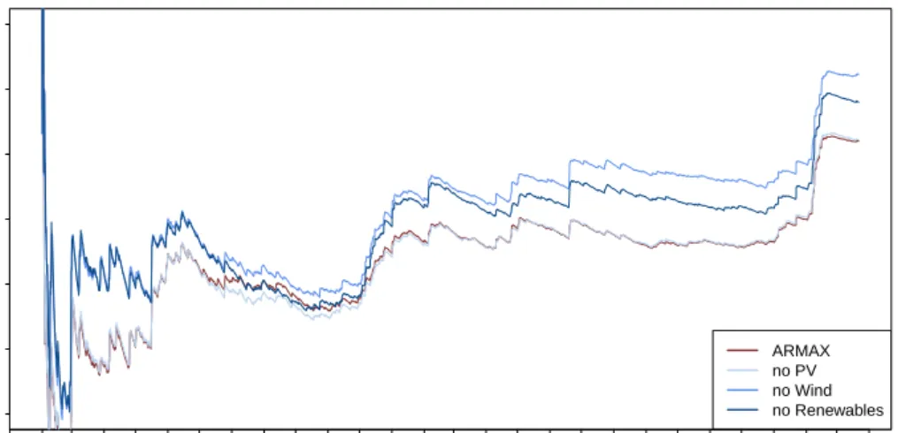
to 8.6 when changing from model (2) to model (4) with externals. Just by including feed-ins from renewables, we achieve an improvement of 3.37 %. Similarly, the RMSE of the Artificial Neural Network decreases from 9.33 in model (3) down to 8.41 in model (6) – a reduction of 9.86 %. Figures 7 and 8 compare the forecasting accuracy across models with all, none or just some exogenous predictors. It can be seen that models which include expected feed-ins from wind power generation achieve the lowest errors. This supports the hypothesis that electricity prices are only marginally driven by solar power, but are highly dependent on wind power. Overall, we see that all models benefit from the inclusion of exogenous predictors substantially.

• Finding 2.Model (7) uses a rolling re-estimation of its parameters. When compared with model (3) with fixed coefficients, we see that the RMSE decreases from 8.60 down to 8.42. Although this reduction of 2.09 % seems small, the actual result is close to the best-performing model (8). Considering that most related work neglects the idea of iteratively updating parameters for each forecasting model, this finding becomes even more relevant.

• Finding 3.Finally, an Artificial Neural Network with exogenous inputs has the best performance. The errors of model (8), with a RMSE of 8.41, as well as a MAE of 5.70, are smaller than the errors of any other model. This finding agrees with related literature, in which Artificial Neural Networks are widely adopted for price forecasting (cf. Aggarwal et al., 2009; Li et al., 2005; Weron, 2006). In addition, we include further models to study various effects. According to model (5), the inclusion of hourly dummies does not result in any improvement. Furthermore, a shorter training set to estimate parameters result in larger errors as shown by model (6). Almost all the models outperform the naïve approach of model (1), which shows a high RMSE of 11.17. Altogether, the results in Table 3 provide an answer to our research question, i. e. forecasting errors abate with the inclusion of our exogenous predictors.

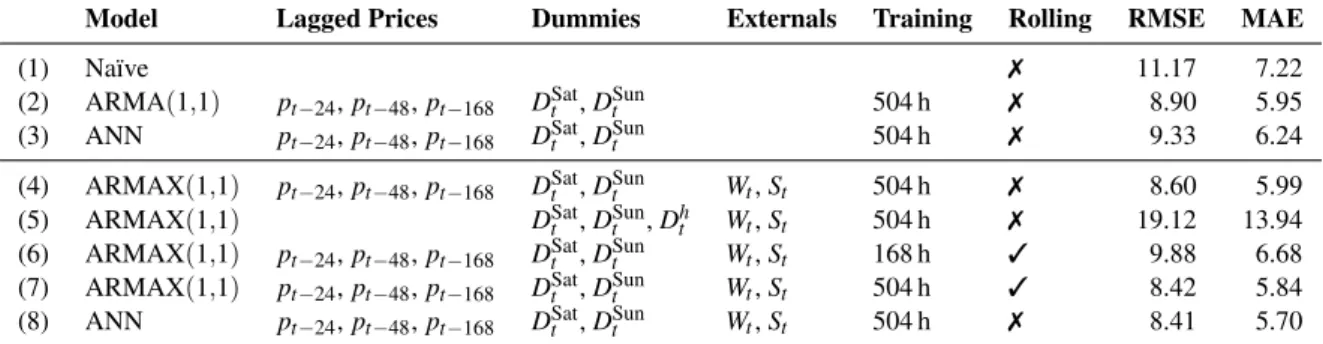
Model Lagged Prices Dummies Externals Training Rolling RMSE MAE

(1) Naïve 7 11.17 7.22

(2) ARMA(1,1) pt−24,pt−48,pt−168 DSatt ,DSunt 504 h 7 8.90 5.95

(3) ANN pt−24,pt−48,pt−168 DSatt ,DSunt 504 h 7 9.33 6.24

(4) ARMAX(1,1) pt−24,pt−48,pt−168 DSatt ,DSunt Wt,St 504 h 7 8.60 5.99

(5) ARMAX(1,1) DSat_t ,DSun_t ,Dh

t Wt,St 504 h 7 19.12 13.94

(6) ARMAX(1,1) pt−24,pt−48,pt−168 DSatt ,DSunt Wt,St 168 h 3 9.88 6.68

(7) ARMAX(1,1) pt−24,pt−48,pt−168 DSatt ,DSunt Wt,St 504 h 3 8.42 5.84

(8) ANN pt−24,pt−48,pt−168 DSatt ,DSunt Wt,St 504 h 7 8.41 5.70

Table 3. Comparison of forecasting accuracy in terms of root mean squared error (RMSE) and mean average error (MAE), measured from February 01, 2010 to March 21, 2012 across various models.

Ultimately, we utilize the Diebold-Mariano test (Diebold & Mariano, 1995) to provide statistical evidence that models including feed-ins from renewables forecast electricity prices more accurately. The null hypothesis tests if methods without feed-ins from renewables are at least as accurate as models lacking these exogenous inputs. When applied to the ARMAX process from model (4), the test statistic returns

3.777 with aP-value of 7.953·10−5. For the Artificial Neural Network, we yield a test statistic of 4.400

Time RMSE 2010−01 2010−04 2010−07 2010−10 2011−01 2011−04 2011−07 2011−10 2012−01 2012−04 6.5 7.0 7.5 8.0 8.5 9.0 9.5 ARMAX no PV no Wind no Renewables

Figure 7. Evolving forecasting accuracy measured by the root mean squared error (RMSE) of ARMAX models with different exogenous inputs over time.

Time RMSE 2010−01 2010−04 2010−07 2010−10 2011−01 2011−04 2011−07 2011−10 2012−01 2012−04 6.5 7.0 7.5 8.0 8.5 9.0 9.5 ANN no PV no Wind no Renewables

Figure 8. Evolving forecasting accuracy measured by the root mean squared error (RMSE) of Artificial Neural Networks with different exogenous inputs over time.

level and, hence, conclude that models including renewables as exogenous predictors are more accurate than models without.

Altogether, the presented approach is subject to certain limitations and implications. First, electricity prices are, nowadays, highly volatile while featuring major price spikes. As a result, these fluctuations put pressure on next-day price forecasts. Second, accurate price forecasts are inevitable when bidding in electricity markets to reduce the value-at-risk and to minimize expenses. Third, a more detailed study reveals that certain periods of extreme weather or policy changes (linked with a price changes that is unpredictable) represent the frontiers of predictive analytics. Nevertheless, the presented approach paves the first steps towards a decision support system.

5 Conclusion

Since the liberalization of electricity markets, market participants can actively participate in the trading of electricity through over-the-counter (OTC) deals, as well as through organized electricity exchanges. This, however, imposes new challenges on participants because they have to actively bid on exchanges or OTC platforms. It is crucial to model and forecast future electricity prices accurately in order to increase profits and to avoid losses from bidding. We utilize a predictive analytics approach by forecasting electricity prices using information on power generation from renewable electricity sources to implicitly incorporate weather conditions. Even though predictive analytics is a sub-field of Information Systems (IS) research, there are not many publications available (Shmueli & Koppius, 2011) that conduct sound predictive analytics research.

As its main contribution, this paper proposes and compares models for forecasting electricity prices using exogenous predictors. Besides weekend dummies, hourly dummies and lagged spot prices, we also incorporate both expected wind and expected solar power generation as external parameters. More specifically, these predictors are embedded in two common electricity price models: an autoregressive-moving-average process with exogenous inputs (ARMAX) and an Artificial Neural Network (ANN). When evaluating the out-of-sample errors, we find strong evidence that the inclusion of expected feed-ins improves forecasting accuracy significantly. Depending on the chosen model, the forecasting accuracy measured as the root mean squared error (RMSE) drops by between 3.37 % and 9.86 %. Moreover, a Diebold-Mariano test provides statistical evidence that the exogenous predictors do indeed lead to superior performance. Improvements in forecasting accuracy are achieved regardless of the model at hand, thus, we can generalize that electricity price modeling benefits from weather parameters. With an augmenting share of renewable energy sources, this effect will accelerate rapidly in the near future, so that including external time series in order to achieve accurate forecasting models will be inevitable.

In future work, we will advance the above methods in two directions. First, our rigorous predictive analysis would benefit greatly from the comparison of additional models such as dynamic regression or regime switching. Second, extending the selection of external predictors would open an avenue for further gains in accuracy. Thus, it might be beneficial to include additional exogenous predictors, such as electricity demand, power plant availability, prices for emission allowances and prices of energy sources.

References

Aggarwal, S. K., Saini, L. M., & Kumar, A. (2009). Electricity price forecasting in deregulated markets: A review and evaluation. International Journal of Electrical Power & Energy Systems, 31(1), 13–22. Bello, A. & Reneses, J. (2013). Electricity Price Forecasting in the Spanish Market using Cointegration

Techniques. In D. B. Jun, R. Fildes, & H. Song (Eds.), The 33rd Annual International Symposium on Forecasting (ISF 2013). ISF electronic proceedings.

Bierbrauer, M., Menn, C., Rachev, S. T., & Trück, S. (2007). Spot and derivative pricing in the EEX power market. Journal of Banking & Finance, 31(11), 3462–3485.

Bishop, C. M. (2009). Pattern recognition and machine learning (8th ed.). Information science and statistics. New York: Springer.

Conejo, A. J., Contreras, J., Espínola, R., & Plazas, M. A. (2005). Forecasting electricity prices for a day-ahead pool-based electric energy market. International Journal of Forecasting, 21(3), 435–462. Contreras, J., Espínola, R., Nogales, F., & Conejo, A. (2003). ARIMA Models to Predict Next-Day

Electricity Prices. IEEE Transactions on Power Systems, 18(3), 1014–1020.

Cruz, A., Muñoz, A., Zamora, J. L., & Espínola, R. (2011). The effect of wind generation and weekday on Spanish electricity spot price forecasting. Electric Power Systems Research, 81(10), 1924–1935.

Diebold, F. X. & Mariano, R. S. (1995). Comparing Predictive Accuracy. Journal of Business & Economic Statistics, 13(3), 253–263.

EEX. (2013). EEX Transparency Platform. Retrieved December 2, 2013, from http://www.transparency. eex.com/

EPEX. (2013). European Power Exchange: Market Data. Paris. Retrieved February 18, 2013, from http://www.epexspot.com/en/market-data

Erni, D. (2012). Day-Ahead Electricity Spot Prices: Fundamental Modelling and the Role of Expected-Wind Electricity Infeed at the European Energy Exchange (Ph.D. School of Management, Economics, Law, Social Sciences and International Affairs, St. Gallen and Switzerland).

Green, R. & Vasilakos, N. (2010). Market behaviour with large amounts of intermittent generation. Energy Policy, 38(7), 3211–3220.

Hastie, T. J., Tibshirani, R. J., & Friedman, J. H. (2013). The elements of statistical learning: Data mining, inference, and prediction (2. ed., corr. at 7th printing.). Springer series in statistics. New York: Springer. Huurman, C., Ravazzolo, F., & Zhou, C. (2012). The power of weather. Computational Statistics & Data

Analysis, 56(11), 3793–3807.

Keles, D., Genoese, M., Möst, D., Ortlieb, S., & Fichtner, W. (2013). A combined modeling approach for wind power feed-in and electricity spot prices. Energy Policy, 59, 213–225.

Knittel, C. R. & Roberts, M. R. (2005). An empirical examination of restructured electricity prices. Energy Economics, 27(5), 791–817.

Kosater, P. (2006). On the impact of weather on German hourly power prices. Retrieved December 2, 2013, from http://www.econstor.eu/handle/10419/26737

Kristiansen, T. (2012). Forecasting Nord Pool day-ahead prices with an autoregressive model. Energy Policy, 49, 328–332.

Li, G., Liu, C.-C., Lawarree, J., Gallanti, M., & Venturini, A. (2005). State-of-the-art of electricity price forecasting. In 2005 CIGRE/IEEE PES International Symposium (pp. 110–119). IEEE.

Misiorek, A., Trueck, S., & Weron, R. (2006). Point and Interval Forecasting of Spot Electricity Prices: Linear vs. Non-Linear Time Series Models. Studies in Nonlinear Dynamics & Econometrics, 10(3), Article 2.

Nogales, F. J. & Conejo, A. J. (2006). Electricity price forecasting through transfer function models. Journal of the Operational Research Society, 57(4), 350–356.

Nogales, F. J., Contreras, J., Conejo, A. J., & Espinola, R. (2002). Forecasting next-day electricity prices by time series models. IEEE Transactions on Power Systems, 17(2), 342–348.

Shmueli, G. & Koppius, O. (2011). Predictive Analytics in Information Systems Research. MIS Quarterly, 35(3), 553–572.

Szkuta, B., Sanabria, L., & Dillon, T. (1999). Electricity price short-term forecasting using artificial neural networks. IEEE Transactions on Power Systems, 14(3), 851–857.

Turban, E. (2011). Business intelligence: A managerial approach (2nd ed.). Boston: Prentice Hall. Weron, R. (2006). Modeling and forecasting electricity loads and prices: A statistical approach. Wiley

Finance Series. Chichester: John Wiley & Sons.

Weron, R. & Misiorek, A. (2008). Forecasting spot electricity prices: A comparison of parametric and semiparametric time series models. International Journal of Forecasting, 24(4), 744–763.

Woo, C., Horowitz, I., Moore, J., & Pacheco, A. (2011). The impact of wind generation on the electricity spot-market price level and variance: The Texas experience. Energy Policy, 39(7), 3939–3944. Xu, H. & Niimura, T. (2004). Short-term electricity price modeling and forecasting using wavelets and

multivariate time series. In Power Systems Conference and Exposition (pp. 858–862). IEEE Power Engineering Society.