Quantifying Landscape Spatial Pattern: What Is the State of the Art? Eric J. Gustafson. Ecosystems, Vol. 1, No. 2. (Mar. - Apr., 1998), pp

(1)

Quantifying Landscape Spatial Pattern: What Is the State of the Art?

Eric J. Gustafson

Ecosystems, Vol. 1, No. 2. (Mar. - Apr., 1998), pp. 143-156.

Stable URL:

http://links.jstor.org/sici?sici=1432-9840%28199803%2F04%291%3A2%3C143%3AQLSPWI%3E2.0.CO%3B2-%23 Ecosystems is currently published by Springer.

Your use of the JSTOR archive indicates your acceptance of JSTOR's Terms and Conditions of Use, available at

http://www.jstor.org/about/terms.html. JSTOR's Terms and Conditions of Use provides, in part, that unless you have obtained prior permission, you may not download an entire issue of a journal or multiple copies of articles, and you may use content in the JSTOR archive only for your personal, non-commercial use.

Please contact the publisher regarding any further use of this work. Publisher contact information may be obtained at http://www.jstor.org/journals/springer.html.

Each copy of any part of a JSTOR transmission must contain the same copyright notice that appears on the screen or printed page of such transmission.

The JSTOR Archive is a trusted digital repository providing for long-term preservation and access to leading academic journals and scholarly literature from around the world. The Archive is supported by libraries, scholarly societies, publishers, and foundations. It is an initiative of JSTOR, a not-for-profit organization with a mission to help the scholarly community take advantage of advances in technology. For more information regarding JSTOR, please contact [email protected].

http://www.jstor.org Wed Jun 27 10:50:04 2007

(2)

Ecosystems (1998) 1: 143-156

Quantifying Landscape Spatial

Pattern: What

Is

the State of the Art?

Eric

J. Gustafson

North Central Forest Experiment Station, 5985 HighwayK, Rhinelander, Wisconsin 54501-91 28, USA

ABSTRACT

Landscape ecology is based on the premise that there are strong links between ecological pattern and ecological function and process. Ecological systems are spatially heterogeneous, exhibiting considerable complexity and variability in time and space. This variability is typically represented by categorical maps or by a collection of samples taken at specific spatial locations (point data). Categorical maps quantize variability by identifying patches that are relatively homogeneous and that exhibit a relatively abrupt transition to adjacent areas. Alter- natively, point-data analysis (geostatistics) assumes that the system property is spatially continuous, making fewer assumptions about the nature of spatial structure. Each data model provides capabilities that the other does not, and they should be considered complementary. Although the concept of patches is intuitive and consistent with much of ecological theory, point-data analysis can answer two of the most critical questions in spatial pattern analysis: what is the appropriate scale to conduct

The quantification of environmental heterogeneity has long been a n objective in ecology (Patil and others 197 1; Pielou 1977). Efforts to develop methods to quantify the spatial heterogeneity of landscapes began more recently (Romrne 1982; Bur- rough 1986; Icrummel and others 1987; O'Neill and others 1988a), but have accelerated so that there are

Received 3 October 1997; accepted 18November 1997. e-mail:[email protected]

the analysis, and what is the nature of the spatial structure? I review the techniques to evaluate categorical maps and spatial point data, and make observations about the interpretation of spatial pattern indices and the appropriate application of the techniques. Pattern analysis techniques are most useful when applied and interpreted in the context of the organism(s) and ecological processes of interest, and at appropriate scales, although some may be useful as coarse-filter indicators of ecosystem function. I suggest several important needs for future research, including continued investigation of scaling issues, development of indices that measure specific components of spatial pattern, and efforts to make point-data analysis more compatible with ecological theory.

K e y words: spatial pattern; index; indices; spatial heterogeneity; patchiness; landscape ecology; scale; geostatistics; autocovariation; spatial models.

now literally hundreds of quantitative measures of landscape pattern that have been proposed to quantify various aspects of spatial heterogeneity (Baker and Cai 1992; McGarigal and Marks 1995). In spite of this, it has been argued that the quantification of spatial heterogeneity remains problematic because of the complexity of the phenomena (Kolasa and Rollo 1991) and because the components of heterogeneity are ill-defined (Li and Reynolds 1994).

There is a rapidly growing demand for measurement and monitoring of landscape-level patterns and processes. This demand is driven by the premise that ecological processes are linked to and can be

(3)

144 E. J. Gustafson

predicted by some (often unknown) ecological pattern exhibited at coarse spatial scales. Although there has been broad acceptance of this premise, the difficulties associated with predicting the response of ecological entities to spatial pattern has led to few definitive tests. For example, in the United States, an ambitious program to sample and monitor landscape patterns nationwide (EMAP) has been proposed (Overton and others 1990; Hunsaker and others 1994), but it remains in a pilot phase due to uncertainty over what to measure and what it might mean (I<epner and others 1995). The US National Forests are currently involved in major planning efforts that include consideration of landscape composition and structure both within each forest and in the surrounding areas (Jensen and others 1996). However, planners often do not have the knowledge to make valid projections of the response of ecological systems to the patterns that will be produced by management activities. Furthermore, information about the historical range of landscape patterns may be difficult to derive. Nevertheless, many conservation and land management organiza- tions, both public and private, now view a landscape perspective as essential for sound resource management (Wallinger 1995; Wigley and Sweeney 1993).

The integration of landscape ecology into re-source management has not been easy, nor is it complete. Many persons without special training in spatial analysis are attempting to calculate and interpret pattern indices. This has been facilitated by the availability of software capable of calculating literally hundreds of indices of landscape pattern from digital maps. The distinction between the heterogeneity that can be mapped and measured and the heterogeneity that is ecologically relevant to the resource being managed is sometimes blurred (Turner 1989). In a n attempt to clarify some of these complexities, I have prepared this review with the following objectives: (a) to describe the state of the art of spatial pattern quantification, (b) to discuss the interpretation of pattern indices, (c) to describe the appropriate application of spatial analysis techniques, and (d) to suggest lines of research that might be particularly useful to meet the needs of researchers and resource managers.

A useful discussion of the state of the art of landscape pattern analysis must begin with definitions since there is considerable inconsistency of terminol- ogy in the literature. Spatial heterogeneity can be defined as the complexity and variability of a system property in time and space (Li and Reynolds 1994).

A system property in this case can be nearly any measurable entity, such as the configuration of the landscape mosaic, plant biomass, annual precipita- tion, or soil nutrient concentrations. Some important measures of heterogeneity are clearly not spatially explicit (for example, number of land types and proportions of these types), but have important spatial effects. Spatial structure is a major subset of the concept of spatial heterogeneity, usually referring to the spatial configuration of the system property. The term spatial pattern has been used extensively in the landscape ecological literature, primarily to describe both the composition and structure of landscapes [for example, see Turner (1989)l. In this review, I use the terms spatial heterogeneiry and spatial pattern synonymously to refer comprehensively to the composition, configuration, and temporal aspects of heterogeneity, and will use the terms structure and configuration when referring solely to the spatial components of heterogeneity.

Pioneers in the quantification of spatial heterogeneity have suggested that heterogeneity can be conceived as an environmental mosaic [see references in Turner ( 1989)], a patterning of ecosystem types in space (Forman and Godron 1986; Icrummel and others 1987; O'Neill and others 1988a), or patchiness (Wiens and others 1993). Spatial heterogeneity is also not static, and neither are ecological processes. Landscapes are usefully visualized as "shifting mosaics" [sensu Bormann and Likens ( 1979)], and ecological systems are characterized by dynamics, disturbance, and change (Huston 1979; Reice 1994). Thus, spatial heterogeneity also has a temporal component, although much less work has been done to capture this aspect of heterogeneity quantitatively [see Dunn and others (1991) and Fahrig (1 992)j.

Heterogeneity is also a function of scale (Wiens 1989; Allen and Hoekstra 1992). The spatial and temporal variation of a system property that can be detected will depend on the spatial and temporal scale at which the property is sampled and the size of the mapping unit. If you were to study an agricultural landscape, for example, you would notice relatively little heterogeneity in vegetation if you stood within a planted field, more heterogeneity if you flew over the fields, woodlots and villages at low altitude, and relatively little if you looked down from a spacecraft. Two primary scaling factors affect measures of heterogeneity: grain is the resolu- tion of the data (minimum mapping unit, pixel size, and time interval) and extent refers to the size of the area mapped or studied, or the time period over

(4)

Table 1. Methods to Represent the Heterogeneity

of a System Property and the Techniques Used to Quantify That Heterogeneity [see also Li and Reynolds ( 1995)]

System Property

Representation Description Quantification

Categorical maps Qualitative variables mapped in space

Nonspatial Composition Number of

categories Proportions Diversity (richness,

evenness)

Spatial Configuration Patch-based indices

Size Shape Patch density Connectivity Fractal dimension Pixel-based indices Contagion Lacunarity

Point data Continuous Trend surface

variables Correlogram

sampled Semivariogram

regularly or Fractal dimension

irregularly in Lacunarity

space Autocorrelation

indices Interpolation (e.g.,

kriging)

which observations were collected (O'Neill and others 1986).

The quantification of spatial heterogeneity re-quires a way to describe and represent variability in space and time. I n practice, spatial heterogeneity is sampled and represented in a number of different ways, each useful for different types of data and having specialized methods for quantification of heterogeneity (Table 1).

Categorical map analysis involves mapping the system property of interest by identifying patches that are relatively homogeneous with respect to that property at a particular scale and that exhibit a relatively abrupt transition (boundary) to adjacent areas (patches) that have a different intensity (or quality) of the system property of interest (Icotliar and Wiens 1990). However, the criteria for defining a patch may be somewhat arbitrary, depending on

Quantifying Landscape Spatial Pattern 145

how much variation will be allowed within a patch, on the minimum size of patches that will be mapped (minimum mapping unit), and the components of the system that are ecologically relevant to the organism or process of interest. Furthermore, a single landscape may exhibit many different patch structures, depending on the system properties measured. For example, very different maps may result if one defines patches based on forest type, stand age, or canopy closure. Thus, the spatial structure may in part be determined by these arbitrary decisions, rather than strictly by the properties of the system itself. As a n example, consider the study of the distribution of aspen in the Wisconsin North- woods. As we attempt to identify and draw boundaries around aspen stands, we are immediately confronted by the question of how much aspen must be present to classify a stand as aspen. If there is a small aspen clone within a hardwood stand, should we map the clone as a n aspen patch? The map we produce would show where aspen was dominant, but would contain little information about the relative abundance of aspen in other parts of the landscape and would imply that all aspen stands were alike. Furthermore, the structure exhibited by the map would at least be partly a n artifact of the mapping decisions made.

Alternatively we might wish to conduct a point- data analysis of this landscape. Point-data analysis assumes that the system property is spatially continuous, making fewer assumptions about the nature of spatial structure. The landscape is sampled to generate spatially referenced information about system variables and is analyzed using geostatistical techniques (so called because of their origin in the geosciences). Here we might measure the abundance of aspen at sample points distributed ran-domly or systematically. The abundance would be highest in aspen stands, but there would be quantification of the abundance of aspen in other forest types as well. In this approach, there are n o explicit boundaries (that is, patches are not delineated), and fewer simplifying assumptions are made concerning the spatial configuration of the system. However, real discontinuities that have ecological relevance (for example, a clear-cut boundary or agricultural edge) are not as easily represented and studied, and the density of sample points affects the spatial properties perceived by analytical tools applied to the landscape.

Because these two approaches to the description of spatial heterogeneity are not combined in most studies, there is a n appearance that they are not complementary. However, each provides a valid way to describe and analyze spatial phenomena,

(5)

146

E. J. Gustafson

and each has strengths and weaknesses that depend o n the ecological system being studied. Patch-based analysis uses a simplified description of the system that is perhaps more amenable to interpretation and is more directly relevant to much of ecological theory than is point-data analysis. However, point- data analysis can answer two of the most critical questions in the analysis of spatial heterogeneity: what is the appropriate scale at which to conduct the analysis, a n d what is the nature of the spatial structure? In many studies, the identification of patches typically reflects a minimum mapping unit that is chosen for compilation and not ecological reasons. Point-data analysis can provide insight into the scale of patchiness, whether there are hierar- chies of scale, and whether the spatial distribution is random, aggregated, or uniform. Many point-data analysis techniques also provide robust capabilities to conduct reliable statistical inference. One of the purposes of this review is to show that categorical and point-data analysis techniques each provide useful and complementary information.

Description of Methods

The fundamental assumption of classical inferential statistical analysis is the independence of observations. However, because the spatial structures we find in nature are commonly patches or gradients, this assumption is usually violated at specific (and usually unknown) scales of sampling. Therefore it is imperative to know something about the degree and scale of spatial dependence in the system being studied. Geostatistics provide methods to both describe spatial structure and to make statistical inferences that are robust in the presence of spatially dependent relationships. Although point data can be used to generate interpolated numerical maps (for example, digital elevation models (DEM), maps of climate variables, and habitat suitability maps), they are typically analyzed to make inferences about some system property in a spatial context.

The method used to represent the spatial variation in the system in digital maps is a n arbitrary construct. Raster maps (constructed of grid cells) represent boundaries as the interface between cells of different classes, so that boundaries must con- form to the underlying lattice structure. This can have marked effects on the delineation of patches, as the lattice structure may affect the contiguity of pixels. Maps constructed of vectors (digitized lines) also characterize boundaries as a sequence of straight lines, but these can be oriented in any direction, and each segment can be very short.

Categorical maps. Quantification of spatial hetero-

geneity is often focused o n categorical (or thematic;

choropleth) maps, in which system properties are represented qualitatively and given arbitrary labels (for example, cover type, soil series name, or habitat quality), although sometimes they are quantitative properties that exhibit discrete spatial discontinuities (for example, forest stand age). Categorical maps tend to ignore the spatial variation within spatial units and trends in system properties across landscapes. A large number of indices have been developed to quantify spatial heterogeneity on categorical maps. These indices fall into two general categories: those that evaluate the composition of the map without reference to spatial attributes, and those that evaluate the spatial configuration of system properties, requiring spatial information for their calculation. Spatial configuration indices are either patch oriented or neighborhood oriented. Patch-oriented indices are calculated considering only a single patch and its edges. Neighborhood- oriented indices are calculated using spatial neighborhoods and may consider complete patches within the neighborhood or only neighboring pixels. An exhaustive list of all published indices is beyond the scope of this review. I present here a representative sample of published indices, with references to more complete descriptions of their calculation.

Composition. Composition is readily quantified,

and is typically described by (a) the number of categories or classes in the map, ( b ) the proportion of each class relative to the entire map, and (c) diversity. The number of classes and their proportions are generated by simple counting algorithms. Diversity measures typically combine two components of diversity: richness, which refers to the number of classes present, and evenness, which refers to the distribution of area among the classes. Examples are the Shannon's (Shannon and Weaver 1949), Simpson's (Simpson 1949), and modified Simpson's (Pielou 1975) diversity indices. The richness and evenness components can also be measured independently (Romme 1982). Dominance is the complement of evenness (evenness = 1 -dominance), indicating the extent to which the map is dominated by one or a few classes (O'Neill and others 1988a) and has been used widely in land-scape ecology research. A less widely known diver- sity index is mosaic diversity as recently proposed by Scheiner (1992). Some composition indices have been spatially referenced by calculating the index within a moving window that is passed across the map. The calculated index value at each point is displayed (Riitters and Wickham 1995; Perera and Baldwin forthcoming), allowing visualization of the spatial variability of the index at a specific scale of resolution (size of the window).

(6)

Spatial configuration. The spatial configuration of

system properties is much more difficult to quantify, and attempts have focused on describing spatial characteristics of individual patches (patch based) and the spatial relationships among multiple patches (neighborhood based). Other metrics evaluate neighborhood properties without reference to patches, using only the pixel representations of system properties. Patch characteristics of an entire landscape are sometimes reported as a statistical summary (for example, mean, median, variance, and frequency distribution) for all the patches of a class (Baskent and Jordan 1995). When the configuration of a single patch type is of particular interest, these analyses are often conducted on simple binary maps, where there are only two classes: the class of interest and all others combined.

Patch-based measures of pattern include size, number, and density of patches. These measures can be calculated for all classes together or for a particular class of interest. Useful edge information may include perimeter of individual patches, total perimeter of all patches of a particular class, the frequency of specific patch adjacencies, and various edge met- r i c ~that incorporate the contrast (degree of dissimi- larity) between the patch and its neighbors (Baker and Cai 1992; McGarigal and Marks 1995). For example, there is less contrast between a mature forest stand and a young stand than there is between the mature stand and a pasture. Patches can take a n infinite variety of shapes, making shape a difficult characteristic to quantify. Most shape indices (including many fractal methods) use a perimeter-area relationship (Forman and Godron 1986; Milne 1991; Riitters and others 1995). Other methods have been proposed-average radius of gyration (Pickover 1990), contiguity (LaGro 199 I ) , linearity index (Gustafson and Parker 1992), and elongation and deformity indices (Baskent and Jordan 1995)- but these have not yet become widely used. A widely used index related to both patch size and shape is core area (interior). Core area is the portion of a patch that is further than some specified distance from a n edge and presumably not influ- enced by edge effects. Some edge effects may extend a relatively short distance into a patch [for example, microclimate (Chen and others 1992)], whereas others may be more pervasive [for example, predation rates o n nesting birds (Robinson 1992)l. The distance used to define the patch core must be derived for a specific organism or process of interest. This distance is usually assumed to be fixed regard- less of the contrast and orientation of the edge adjacent to the core. Baskent and Jordan (1995) describe a technique that uses a varying edge dis-

tance to determine core area. GISFrag is a related index (Ripple and others 199 1) that is calculated by finding the average distance to the nearest edge of all the pixels of the class of interest. It is used as an index of patch fragmentation and can function equally well as a landscape-level or patch-level index.

The interspersion and juxtaposition index developed by McGarigal and Marks ( 1 995) measures the extent to which patch types (patches of different classes) are interspersed. This patch-based index is conceptually similar to the pixel-based contagion index (see below), but rather than evaluating pixel adjacencies, the interspersion index evaluates only patch adjacencies. Whereas contagion measures the "clumpiness" of maps, this index measures the juxtaposition of patch types.

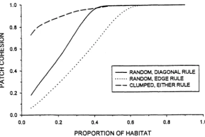
Patch cohesion (PC) was recently proposed by Schumaker (1996) to quantify the connectivity of habitat as perceived by organisms dispersing in binary landscapes. Because the behavior of PC has not been described over the full range of habitat proportions, I digress momentarily to illustrate its potentially useful features. I examined PC on maps where habitat cells were assigned at random, calculating PC by using all patches on the map by

where p is patch perimeter, a is patch area, and N is the number of pixels in the map. It is well known that, on random maps, patches gradually coalesce as the proportion (p) of habitat cells increases, forming a large, highly connected patch that spans the lattice at a critical proportion (p,) (Stauffer 1985). The p, varies with the rule used to connect cells to delineate a patch: when cells must share a common edge to be considered connected, p, = 0.59, and when they need only touch at a comer, p, = 0.41 (Stauffer 1985). The PC index has the interesting property of increasing monotonically until a n asymptote is reached near p, (Figure 1 ) . I also examined PC on maps generated by randomly placed clumps of habitat [as in Gustafson and Parker (1992)l. Here the slope of the increase was much less, but asymptote was still reached near p, (Figure 1 ) .

Pattem indices that examine a spatial neighborhood have either a patch orientation or a pixel orientation. Patch-level neighborhood indices usually consider patches o n a binary map. The simplest of these is isolation, which is calculated as the distance to the nearest neighboring patch of the same class. Some indices identify a neighborhood of limited extent around a focal patch (usually a buffer

(7)

148 E. J. Gustafson

-

RANDOM, DIAGONAL RULE

... RANDOM, EDGE RULE

--

CLUMPED, EITHER RULE

0.0

4

0.0 0.2 0.4 0.6 0.8 1.0

PROPORTION OF HABITAT

Figure 1. Patch cohesion (Schumaker 1996) as a function

of proportion of habitat on randomly generated maps

( 100 X 100 cells). Habitat was assigned to cells independently (random) or in clumps (clumped). Patches were delineated by one of two rules: ( a ) cells must share a common edge to be considered connected (edge rule), or (b) cells need only touch at a corner (diagonal rule).

some specific distance around the edge of each patch), and the index is calculated based o n the characteristics of the patches found within that buffer (neighborhood). These indices were developed primarily to predict relative connectivity of habitat islands. A simple example is the average isolation of all patches within the neighborhood (Gustafson and Parker 1992). Some explicitly consider physical connections (for example, corridors or hedgerows) and are supported by network theory (Lowe and Moryadas 1975; Lefkovitch and Fahrig 1985). Others are based on island-biogeography theory (MacArthur and Wilson 1967) and incorporate both island (patch) size and isolation [isolation index (Whitcomb and others 1981) and proximity index (Gustafson and Parker 1992)l. Verboom and others ( 199 1) developed a connectivity index in the context of metapopulation theory (Levins 1970).

The most commonly used pixel-based neighborhood index is contagion (O'Neill and others 1988a), designed to quantify both composition and configuration. Li and Reynolds (1993) have corrected a n error in the original formula, and Riitters and others (1996) have clarified subtleties in the way adjacencies are tabulated. Contagion ignores patches per se

and measures the extent to which cells of similar class are aggregated. The index is calculated using the frequencies with which different pairs of classes occur as adjacent pixels on the map. The index typically does not distinguish differences in aggregation that may exist for different classes, but summa- rizes the configuration of all classes. Contagion is sometimes mistakenly used as a surrogate for aggre-

gation of a specific type (for example, forest), pointing out the need for care in the interpretation of the contagion index. [Alternative methods are available for calculating class-specific contagion measures (Pastor and Broshart 1990; Gardner and O'Neill 199 1) .] Contagion has also been mapped by display- ing the contagion value calculated within a moving window (Riitters and Wickham 1995; Perera and Baldwin forthcoming). The use of the contagion index is appealing because it appears to summarize the overall clumpiness of maps effectively, but is problematic because it is a single-valued index used to represent complex interacting patterns.

Lacunarity analysis is a multiscale method used to determine the heterogeneity (or texture) of a system property represented as a binary response in one, two, or three dimensions (Plotnick and others 1993, 1996). The technique uses a gliding box (moving window) algorithm to describe the probability distribution of the class of interest as the box is passed over the data (a map, a transect, or points). Valuable insight into the spatial heterogeneity of the system and the domains of the scale of variation in that pattern can be achieved by using a number of box sizes and plotting lacunarity as a function of box size.

Point-data analysis. In contrast to techniques ap-

plied to thematic maps of categorical data, point- data analysis is applied to data collected by sampling rather than to maps. The analysis assumes that the system property varies continuously in space, and applies mathematical techniques for modeling gradual spatial change (Journel and Huijbregts 1978; Davis 1986; Rossi and others 1992; Burrough 1995). These techniques are not constrained by the need to delineate boundaries o n the map and are very different from the techniques applied to categorical maps. Only a superficial discussion of these techniques is possible here. The interested reader is referred to excellent reviews by Legendre and For- tin (1989), Turner and others (1991), Rossi and others (1992), and Burrough (1995).

Trend suface. One simple way to estimate the gradual, broad-scale spatial variation (trend) in a system property is to fit a surface to the data using regression techniques (trend-surface analysis). The estimated model represents the systematic trend in the data, and the deviations from the surface represent the random component of the system. For example, biomass accumulation rates at a regional scale might exhibit a spatial trend related to growing degree-days. Although easy to calculate, this technique must be used with care due to a number of problems (Burrough 1995). Regression techniques

(8)

are susceptible to outliers when data points are few, edge effects can be severe with higher-order equa- tions, and the assumption of spatially independent, normal residuals is often violated. Also, finding a trend has little value unless it has a physical or ecological explanation. Trend surface analysis is useful to remove large-scale trends to enable investigation of other, more-fine-scale structures (Legen- dre and Fortin 1989).

Autocorrelation. Often the variation in a system

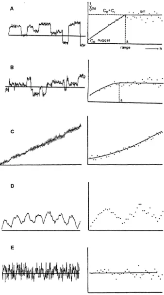
property is such that points close together tend to be more similar than points farther apart, but the pattern is not as simple as would be implied by a trend surface. The degree of similarity (or covariance) between observations separated by varying distances (lags) is computed. The autocovariance for a lag (t) is the covariance among all observations that are separated by a distance of t (Davis 1986). Plotting the autocorrelation (autocovariance normal- ized with respect to the variance of the observa- tions) against t gives the correlogram, which allows visualization of the spatial structure of the system property (Legendre and Fortin 1989) and is useful to determine the grain and extent of repeated spatial pattern (Turner and others 199 1). Semivariograms are conceptually related to correlograms, plotting semivariance against lag distance. The semivariance is the sum of squared differences between all points that are separated by distance t. If the compared points are increasingly different as t increases, the semivariance increases. As t increases, the points eventually become unrelated to each other so that the semivariance equals the average variance of all samples, and the slope becomes zero (Figure 2 ) . The semivariogram can be used to estimate the scale(s) of patchiness of a mosaic (Turner and others 199 1 ) . For example, if we imagine that the semivariogram in Figure 2A represents vegetation height sampled on a transect, a good estimate of the scale of patchiness of height might be the range ( a ) of the semivariogram.

Anisotropy (autocorrelation that differs in different directions) is often found in ecological data because spatial patterns are sometimes produced by directional geophysical phenomena. Anisotropy can be detected by computing the autocorrelation among points oriented to each other in specific directions and comparing them (Legendre and Fortin 1989). As a n example, Burrough (1995) used the semivariogram to analyze the spatial variation in soil texture and found patchiness at scales between 600 and 950 m in a north-south direction, but patches were longer than 1800 m in a n east-west direction.

nugget i a

"F

range

-

h

Figure 2. Some forms of semivariograms right and the possible forms of variation they describe left. In a typical form of the semivariogram A, the range ( a )is the distance

( h )at which the semivariance [ y ( h ) ]levels out, and this level is known as the sill, which is theoretically equal to the variance of the system. The nugget variance (Co) represents random error. B The same as A, but with no single clearly defined distance between abrupt changes. C

A linear trend produces a semivariogram whose slope

increases with h. D A periodic signal produces a cyclic sernivariogram. E Structureless variation or "noise" results in a semivariogram that is 100% nugget variance. Adapted from Burrough (1995).

The quantification of spatial pattern is not as easy as the proliferation of indices might suggest. Measures of spatial pattern often incorporate multiple aspects of composition and pattern in their calculation,

(9)

150 E. J. Gustafson

making interpretation fraught with pitfalls. There is seldom a one-to-one relationship between index values and pattern (that is, several configurations may produce the same index value).

Domains of scale appear to exist in which a relationship established at a particular scale may be reliably extrapolated at similar scales, but may break down when applied at very different scales (Icrum- me1 and others 1987; Urban and others 1987; Wiens and others 1993). For example, least flycatchers and American redstarts are negatively associated in forests of the northeastern United States, but are positively associated at a regional scale (Sherry and Holmes 1988). Because the transition between domains of scale is not intuitively obvious, care must be exercised about the scale to which research findings are applied. Geostatistical techniques (Jour- nel and Huijbregts 1978; Legendre and Fortin 1989; Turner and others 1991; Rossi and others 1992) and fractal analysis (Mandelbrot 1977) have shown the potential to identify transitions between landscape pattern scale domains (Palmer 1988; Milne 1991; Icrummel and others 1987).

Much of the thinking about spatial heterogeneity in ecology and conservation biology has been shaped by island-biogeography theory (MacArthur and Wil-son 1967). This has resulted in essentially a binary model of habitat: suitable habitat and unsuitable habitat (Wiens 1994). We have learned that for binary maps the predominant determinant of spatial pattern is proportion of the class of interest (O'Neill and others 1988b; Gustafson and Parker 1992). This compositional characteristic determines the probable range of many patch configuration characteristics. Often, knowing the proportion of a type of interest tells you almost as much as knowing many other measures of heterogeneity. If proportion is low, generally the patches are small and isolated, and do not have enough area to form convoluted shapes. For example, the most significant explanatory variable used to predict the quality of a landscape as wild turkey habitat in Indiana was proportion of forest (Gustafson and others 1994). Cowbird parasitism and nest predation rates on forest birds in the midwestern United States were negatively correlated with proportion of forest cover o n nine landscapes (Robinson and others 1995), and forest fragmentation indices were correlated with proportion of forest. Andren (1994) reviewed studies of birds and small mammals and discovered that when the proportion of suitable habitat was less than 10%-30%' the effects of patch area and isolation became greater than effects expected from habitat loss alone.

We have also learned that many indices used to quantify spatial heterogeneity are correlated (O'Neill and others 198Sa; Riitters and others 1995) and exhibit statistical interactions with each other (Li and Reynolds 1994). Furthermore, many indices are confounded, that is, they appear to measure multiple components of spatial pattern (Li and Reynolds 1994; Riitters 1995). Some have argued the desirability of indices that combine multiple components of pattern into a single value to reduce the number of variables carried in a multivariate analysis (Riitters and others 1996; Scheiner 1992). Others have argued that it is difficult enough to interpret indices that measure a single component of spatial pattern, and that any method to quantify spatial pattern must be examined theoretically and tested under controlled conditions (Li and Reynolds 1994). A proposed solution is to describe fundamental components of spatial pattern that are independent and develop a suite of metrics to measure those components (Li and Reynolds 1994; Riitters and others 1995). A first approximation of those factors has recently appeared in the literature. Li and Reynolds ( 1995 ) divided spatial heterogeneity into five components using theoretical considerations: compositional components are ( a ) number of types and (b) proportion of each type; and spatial components are (c) spatial arrangement of patches, (d) patch shape, and ( e ) contrast between neighboring patches. Riitters and others (1995) conducted a factor analysis of 55 indices of spatial pattern calculated for 85 maps of land cover and identified five independent factors that they have interpreted as (a) average patch compaction, (b) overall image texture (pixel distributions and adjacencies), (c) average patch shape, (d) patch-perimeter scaling (fractal measures), and (e) number of types. McGari- gal and McComb (1995) conducted a principle component analysis of 30 indices calculated for late-sera1 forest landscapes in the northwestern United States and identified three principal components: ( a ) patch shape and edge contrast, (b) patch density, and (c) patch size.

It is often useful to explore the response and sensitivity of indices to variation i n heterogeneity (Haines-Young and Chopping 1996). Neutral models (Gardner and others 1987; Gardner and O'Neill 1991) have been used extensively for this purpose (Li and Reynolds 1993; Gustafson and Parker 1992; Milne 1992) because they control the process gener- ating the heterogeneity, allowing unconfounded links between variation in heterogeneity and the behavior of the index. Additionally, they are used to generate patterns expected in the absence of a hypothesized process that can be compared with

(10)

those produced by the process under study (With and Icing 1997). An understanding of the response of a n index to a neutral model of a process can quickly illuminate what might otherwise be intrac- table.

Critical to any study of the link between spatial pattern and ecological process is to remember the temporal dynamics of pattern. Land-use mosaics change at various temporal and spatial scales. Crops are rotated o n a n annual basis in agricultural landscapes, and silvicultural practices and regeneration significantly change forested landscapes over de-cades. Human development and land abandonment have dramatically changed many landscapes over a period of decades and centuries. Fire and wind disturbances reshape vegetation mosaics over a period of decades and centuries. In seeking to establish the spatial pattern needed to support an ecological process, it is imperative to understand that a range of pattern conditions must be identified. Very few heterogeneity indices include a measure of temporal variation. This is a serious defi- ciency because it encourages a static view of nature and a n unrealistic concept of change in natural systems (Huston 1994). Because change and variability are part of ecological systems, an understanding of what constitutes a significant change in ecological heterogeneity is critical to understanding the conse- quences for ecological processes. Statistical techniques can detect significant changes in the mean of a pattern index with known variation, but ecologically significant change is much more difficult to assess. For example, a number of patternlprocess relationships appear to be threshold phenomena (Birney and others 1976; O'Neill and others 1989; With and Crist 1995; Wiens and others 1997), where only changes in pattern near the threshold are ecologically important. Also, the ecological significance of pattern measured at one point in time is difficult to assess without a n understanding of the historical variability

of

that pattern.

The proper application of landscape pattern analysis is not trivial. Perhaps the most critical step is to identify properly the scale of the heterogeneity

(patchiness) of the landscape, so that subsequent analyses will be conducted at an appropriate scale. This may require a geostatistical andlor fractal analysis, although the scale of patchiness may be obvious in some systems. Although critical, this step is almost always omitted because it usually involves collecting extra (point) data and conducting spatial statistical analyses with unfamiliar (to many) tech-

niques. If maps are not available at the scale identified as appropriate, compilation of a new landscape map may be required. Considerable thought must also be given to the scale at which the ecological process being studied operates, andior the scale at which the organism(s) being studied perceives (or responds to) the heterogeneity of the landscape (Wiens 1989).

The concept of ecological neighborhoods (Addi- cott and others 1987) has not been widely applied, but could be useful. The concept is centered on a n ecological process and/or organism, and an ecological neighborhood is defined by the time period and the spatial area in which the organism or process interacts with the environment. Patchiness is then measured relative to the size of the neighborhood. For example, relative patch size is the ratio of patch size to neighborhood size, and relative patch duration is the ratio of patch duration to the time scale of the neighborhood. This conceptual framework also serves as a reminder that the pattern and process we measure is but a snapshot of a dynamic system.

In studies linking pattern and process, it is critical [o measure pattern and process at the same spatial scale (that is, both grain and extent). Many measures of heterogeneity are made using a grain determined by data collection or storage methods (for example, resolution of satellite imagery or minimum mapping unit of a GIs layer). Because the collection of landscape data is expensive, these sources are often used out of necessity. Data are routinely resampled to change the grain, although this should be done with caution because resam- pling introduces spatial errors (Turner and others 1989) and produces nonspatial statistical effects in indices that depend on pixel adjacencies or patch counts (Haines-Young and Chopping 1996). Map boundaries usually truncate patches, so map extent can affect patch measures. Considerable thought should be given to the appropriate grain and extent to represent accurately the ecological neighborhood being studied. This task is somewhat easier for simulation studies, as the spatial information used by the model (process) can be used to measure the pattern. However, this precaution is sometimes overlooked. For example, Schumaker (1996) calculated indices of habitat connectivity by using Land- sat multispectral scanner data (0.32 ha, square pixels) and related them to the results of a dispersal model that operated o n a hexagonal grid with cell sizes ranging from 12 to 331 ha. The grain with which system properties are represented has a profound effect on many indices, particularly pixel- based measures and those that incorporate patch edges (Haines-Young and Chopping 1996).

(11)

152 E. J. Gustafson

It also crucial to understand what a n index actually measures relative to the process under consideration. This cannot be overemphasized. Some indices appear intuitive, but their behavior displays subtleties (for example, contagion) that can mislead interpretation. Many indices measure multiple aspects of pattern (for example, diversity indices, proximity index, patch cohesion, and many edge measures). These present difficult interpretation problems that can only be overcome by careful consideration of how the metric is calculated, the characteristics of the map representing the pattern, and a n understanding of the behavior of the index as the pattern of interest changes. Simultaneous consideration of several indices that measure specific components of heterogeneity may be instructive. As Li and Reynolds ( 1994) warn, it is important to perceive correctly the spatial and nonspatial (composition) elements being measured.

Very few pattern indices produce values that are useful by themselves. Their most instructive use is in comparing alternative landscape configurations, either the same landscape at different times or under alternative scenarios, or different landscapes represented by using the same mapping scheme and at the same scale. Pattern indices are also commonly used as independent variables in models attempting to establish a link between spatial pattern and ecological process. The relationship between ecological processes and absolute values of indices is rarely known, although sometimes the relative response of ecological systems to the direction of change in index values is understood.

Many patch-based indices are commonly summa- rized for a n entire landscape by calculating the mean and variance of the index for all patches of each class. This may be misleading when the distribution of patch sizes is greatly skewed toward smaller patch sizes, as is typically the case. Area- weighted means or medians may provide better estimates of central tendency. Another common approach to landscape analysis involves identifying a subset of the landscape around a patch or study site of particular interest, and indices are calculated for that subset to quantify the landscape context of the site. Composition indices are most commonly used, but some patch-based measures may be calculated. Patch-based measures will be affected by edges that truncate patches, and this problem will be severe for subsets that are small relative to the size of patches.

When investigating the relationship between spatial pattern and ecological process, there is always a temptation to calculate as many indices of pattern as possible and look for relationships. The availability

of software to automate the quantification of spatial pattern makes this temptation difficult to resist. It is very rare that some ecological mechanism for a relationship between pattern and process can not be proposed, and explanatory studies should be focused by these putative relationships. Only the most preliminary exploratory studies should embark on "fishing" expeditions and then only with a clear understanding of potential mechanisms driving the process and explicit knowledge of what the pattern indices are measuring.

In 1989, John Wiens challenged researchers to make scaling issues a primary focus of research efforts. Little progress has been made due to the difficulty of scaling problems. Nevertheless, the successful application of research findings depends critically on both identifying the appropriate scale for the application and the ability to extrapolate findings across scales.

Much of the need for spatial pattern indices is driven by the desire to predict the response of some ecological entity (for example, fire, organism, or nutrient flux) to the spatial heterogeneity of a managed landscape. These responses are often complex, caused by interactions between various components of heterogeneity and scale. Many of the indices that have been developed are a n attempt to capture the elements of pattern that are important to a specific ecological entity [for instance, connectivity (Verboom and others 1991) or proximity (Gustafson and Parker 1994)l. For example, Ver- boom and others (1991) developed a connectivity index to quantify patch isolation that was relevant to a metapopulation of European nuthatches. The index significantly improved predictions of patch occupancy by nuthatches. However, indices developed for specific purposes or systems are by definition not very general, and their usefulness may be limited to narrow applications. Nevertheless, with careful application, linking specific ecological processes with special indices may provide the ability to predict those processes by measurement of spatial heterogeneity.

There also appears to be some impetus to develop indices that capture all relevant aspects of heterogeneity in a single value (Scheiner 1992; Riitters 1996), or a suite of indices where each index measures exactly one component of spatial heterogeneity (Li and Reynolds 1994). This may be desir- able, but perhaps is not sufficient. It is unlikely that all ecological processlpattern relationships can be adequately described by using a small suite of

(12)

metrics. Also, it must be verified that a combination of indices can adequately capture the heterogeneity to which specific species or ecological processes are related. It should also be mentioned that it may not be possible to know all the important pattern1 process relationships, and that general indices may be useful even when there is not a n explicit link to specific species or ecological processes. Such a view is consistent with the coarse-filter strategy to main- tain biodiversity proposed by Hunter ( 1990).

The effects of the methods we use to characterize spatial heterogeneity and relate it to ecological function have been inadequately explored. For example, we have become comfortable with characterizing landscapes as thematic (categorical) maps, and most of the commonly used pattern quantification methods are designed for use with categorical data. It is well established, however, that many ecological and environmental conditions are best characterized as gradients (Chen and others 1992). Conditions within "patches" are never completely homogeneous, and even relatively high-contrast boundaries (edges) between habitat types are commonly conceived as ecotones .(that is, a gradient) (Fortin 1994; Fortin and others 1996). More research is needed to develop our ability to characterize and quantify spatial point data to make them compatible with current theory couched in a patch framework and to interpret the results of these analyses reliably.

This review has highlighted the pervasiveness of the island paradigm in studies of spatial pattern (and ecological process for that matter). With the excep- tion of edge and adjacency measures, all indices calculated for categorical maps are based o n a binary patch model. However, habitat patches usually exist in a complex landscape mosaic, and dynamics within a patch are affected by external factors related to the structure of the mosaic (Wiens 1994; Gustafson and Gardner 1996). Although the patch model is best suited to many landscape studies, some landscape mosaics are better represented as gradients (or continuously varying surfaces) of system properties. The island model has sometimes been forcibly im- posed o n the study of such systems (Wiens 1994), and this has been a conceptual impediment to progress in our ability to understand and model the link between spatial pattern and ecological process in systems without discrete boundaries.

The available techniques for the study of continuously varying systems (point-data analysis) have not been widely embraced. This may be partly

because the methods are more complex, and their interpretation is less intuitive than patch models. It is also not widely appreciated that these methods lend themselves to powerful tests of spatial heterogeneity hypotheses (Legendre and Fortin 1989; Turner and others 1991). Many of these methods provide information o n the "patchiness" of the system or can be used to delineate "patch" boundaries [for example, constrained clustering (Legendre and Fortin 1989)], pointing the investigator back toward a less arbitrary patch model [see Fortin and Drapeau ( 1995)l. Spatial autocorrelation should be assumed for most ecological data. Investigators should test for spatial autocorrelation and describe the spatial structure by using maps and spatial structure functions (for example, correlograms and variograms). Such analyses seem necessary to choose the appropriate scale for landscape analysis (patch- based or continuous) and to avoid violating assumptions of the analysis methods.

Several guidelines for sound analysis of spatial heterogeneity have emerged from this review: (a) Get the scale right. This includes determining the scale of patchiness and the hierarchical structure by using geostatistical or fractal techniques. Equally important is to understand the scale of the ecological process(es) of interest. This information determines how the system should be represented (for example, point data or map, categorical or continuous, minimum mapping unit, resolution, and extent). ( b ) Choose the analysis method based on the objectives of the analysis and the spatial characteristics of the system property of interest. (c) Choose metrics by considering the heterogeneity that is relevant to the ecological process of interest. Be- come familiar with the behavior of indices as heterogeneity changes, building neutral models if necessary. When possible, calculate multiple indices that measure the same component of heterogeneity to increase the reliability of the measure of heterogeneity. ( d ) Formulate a theoretical relationship between a n index and the ecological process so that empirical evidence can be rationally related to the results of the analysis. Remember that heterogeneity indices function as surrogate measures of certain ecological conditions, and empirical or theoretical links between them are necessary.

In

summary, spatial heterogeneity indices represent a link between pattern and process. Patch- based landscape analyses have been the primary focus of landscape ecological analysis, and are in- deed appropriate for a majority of ecological questions. However, the appropriate spatial and temporal scales at which these analyses are applied should be determined by geostatistical analysis. Geostatisti-

(13)

154

E. J. Gustafson

cal alternatives to a patch-based approach should be considered when the system property varies gradually in space andlor time. These techniques are most useful when applied and interpreted in the context of the organism(s) and ecological processes of interest, and at appropriate scales, although some may be useful as coarse-filter indicators of ecosystem function [sensu Hunter (1990)l.

I thank Marie-JosPe Fortin, Curt Flather, and two anonymous reviewers for critical reviews that greatly improved the manuscript.

R E F E R E N C E S

Addicott JF, Aho JM, Antolin MF, Padilla DI<, Richardson JS, Soluk DA. 1987. Ecological neighborhoods: scaling environmental patterns. Oikos 49:340-6.

Allen TFH, Hoekstra TW. 1992. Toward a unified ecology. New York: Columbia University.

Andren H. 1994. Effects of habitat fragmentation o n birds and mammals in landscapes with different proportions of suitable habitat: a review. Oikos 71:355-66.

Baker WL, Cai Y. 1992. The r.le programs for multiscale analysis of landscape structure using the GRASS geographical information system. Landscape Ecol7:291-302.

Baskent EZ, Jordan GA. 1995. Characterizing spatial structure of forest landscapes. Can J For Res 25:183049.

Birney EC, Grant WE, Baird DD. 1976. Importance of vegetative cover to cycles of Microtus populations. Ecology 57: 1043-5 1. Bormann FH, Likens GE. 1979. Pattern and process in a forested

ecosystem. New York: Springer-Verlag.

Burrough PA. 1986. Principles of geographic information systems for land resources assessment. Oxford: Clarendon.

Burrough PA. 1995. Spatial aspects of ecological data. In: Jong- m a n RHG, ter Braak CJF, van Tongeren OFR, editors. Data analysis in community and landscape ecology. Cambridge: Cambridge University. p 2 13-5 1.

Chen J, Franklin JF, Spies TA. 1992. Vegetation responses to edge in old-growth Douglas-fir forests. Ecol Appl2:387-96. Davis JC. 1986. Statistics a n d data analysis in geology. New York:

J o h n Wiley and Sons.

D u n n CP, Sharpe DM, Guntenspergen GR, Stearns F, Yang Z. 199 1. Methods for analyzing temporal changes i n landscape pattern. In: Turner MG, Gardner RH, editors. Quantitative methods i n landscape ecology. New York: Springer-Verlag.

p 173-98.

Fahrig L. 1992. Relative importance of spatial and temporal scales i n a patchy environment. Theor Popul Biol41:300-14. Forman R'IT, Godron M. 1986. Landscape ecology. New York:

J o h n Wiley a n d Sons.

Fortin M-J. 1994. Edge detection algorithms for two-dimensional ecological data. Ecology 75:956-65.

Fortin M-J, Drapeau P. 1995. Delineation of ecological boundaries: comparison of approaches and significance tests. Oikos 72:323-32.

Fortin M-J, Drapeau P, Jacquez GM. 1996. Quantification of the spatial co-occurrences of ecological boundaries. Oikos 77: 5 1-60.

Gardner RH, iMilne BJ. Turner MG, O'Neill RV. 1987. Neutral models for the analysis of broad-scale landscape pattern. Landscape Ecol 1:19-28.

Gardner RH, O'Neill RV. 199 1. Pattern, process, and predictabil- ity: the use of neutral models for landscape analysis. In: Turner MG, Gardner RH, editors. Quantitative methods in landscape ecology. New York: Springer-Verlag. p 289-307

Gustafson EJ, Gardner RH. 1996. The effect of landscape heterogeneity o n the probability of patch colonization. Ecology 77:94-107.

Gustafson EJ, Parker GR. 1992. Relationship between landcover proportion and indices of landscape spatial pattern. Landscape ECOI 7:101-10.

Gustafson EJ, Parker GR. 1994. Using an index of habitat patch proximity for landscape design. Landscape Urban Plann 29: 117-30.

Gustafson EJ, Parker GR, Backs SE. 1994. Evaluating spatial pattern of wildlife habitat: a case study of the wild turkey

(Meleagrisgaliopavo). Am Midl Nat 13 1:24-33.

Haines-Young R, Chopping M. 1996. Quantifying landscape structure: a review of landscape indices and their application to forested landscapes. Prog Phys Geogr 20:418-45.

Hunsaker CH, O'Neill RV, Jackson BL, Timmins SP, Levine DA, Norton DJ. 1994. Sampling to characterize landscape pattern. Landscape Ecol 9:207-26.

Hunter ML Jr. 1990. Coping with ignorance: the coarse-filter strategy [or maintaining biodiversity. In: I<olirn I<, editor. Balancing on the brink of extinction. Washington (DC): Island Press. p 266-8 1.

Huston MA. 1979. A general hypothesis of species diversity. Am Nat 113:81-101.

Huston MA. 1994. Biological diversity: the coexistence of species on changing landscapes. Cambridge: Cambridge University. Jensen ME, Bourgeron P, Everett R, Goodman I. 1996. Ecosystem

management: a landscape ecology perspective. J Am Water Resour Assoc 32:203-16.

Journel AG, Huijbregts CJ. 1978. Mining geostatistics. London: Academic.

I<epner WG, Jones I<B, Chaloud DJ. 1995. Mid-Atlantic landscape indicators project plan. Washington (DC): Office of Research and Development; EPAi620lR-951003.

I<olasa J, Rollo CD. 1991. The heterogeneity of heterogeneity: a glossary. In: Kolasa J, Pickett STA, editors. Ecological heterogeneity. New York: Springer-Verlag. p 1-23.

Icotliar NB, Wiens JA. 1990. Multiple scales of patchiness and patch structure: a hierarchical framework for the study of heterogeneity. Oikos 59:253-60.

Krummel JR, Gardner RH, Sugihara G, O'Neill RV, Coleman PR. 1987. Landscape patterns in a disturbed environment. Oikos 48:32 1-4.

LaGro J Jr. 1991. Assessing patch shape in landscape mosaics. Photogrammetric Eng Remote Sens 57:285-93.

Lefkovirch LP, Fahrig L. 1985. Spatial characteristics of habitat patches and population survival. Ecol Model1 30:297-308. Legendre P, Fortin M-J. 1989. Spatial pattern and ecological

analysis. Vegetatio 80:107-38.

Levins R. 1970. Extinction. In: Gerstenhaber M, editor. Some mathematical problems in biology. Providence: American Math- ematical Society. p 77-107.

Li H, Reynolds JF. 1993. A new contagion index to quantify spatial patterns of landscapes. Landscape Ecol8: 155-62.

(14)

Li H, Reynolds JF. 1994. A simulation experiment to quantify spatial heterogeneity in categorical maps. Ecology 75:2446-55. Li H, Reynolds JF. 1995. On definition and quantification of

heterogeneity. Oikos 73:280-4.

Lowe JC, Moryadas S. 1975. The geography of movement. Boston: Houghton Mifflin.

MacArthur RH, Wilson EO. 1967. The theory of island biogeography. Princeton: Princeton University.

Mandelbrot BB. 1977. Fractals, form, chance and dimension. San Francisco: WH Freeman.

McGarigal K, Marks BJ. 1995. FRAGSTATS: spatial pattern analysis program for quantifying landscape structure. Portland (OR): USDA Forest Service, Pacific Northwest Research Sta- tion; General Technical Report PNW-GTR-35 1.

McGarigal K, ~McComb WC. 1995. Relationships between landscape structure and breeding birds in the Oregon Coast Range. Ecol Monogr 65:235-60.

Milne BT. 1991. Lessons from applying fractal models to iand- scape patterns. In: Turner MG, Gardner RH, editors. Quantita- tive methods in landscape ecology. New York: Springer-Verlag. p 199-235.

Milne BT. 1992. Spatial aggregation and neutral models in fractal landscapes. Am Nat 139:32-57.

O'Neill RV, DeAngelis DL, Waide JB, Allen TFH. 1986. A hierarchical concept of ecosystems. Princeton: Princeton University. O'Neill RV, Johnson AR, King AW. 1989. A hierarchical frame-

work for the analysis of scale. Landscape Ecol 3:193-205. O'Neill RV, Krummel JR, Gardner RH, Sugihara G, DeAngelis DL,

Milne BT, Turner MG, Zygmunt B, Christensen SW, Dale VH, Graham RL. I988a. Indices of landscape pattern. Landscape Ecol 1:153-62.

O'Neill RV, Milne BT, Turner MG. Gardner RH. 1988b. Resource utilization scales and landscape pattern. Landscape Ecol 2: 63-9.

Overton WS. White D, Stevens DL Jr. 1990. Design report for EMAP Environmental Monitoring and Assessment Program. Corvallis (OR): US Environmental Protection Agency, Environ- mental Research Laboratory; EPA160013-9 1 105 3.

Palmer MW. 1988. Fractal geometry: a tool for describing spatial patterns of plant communities. Vegetatio 75:9 1-102.

Pastor J, Broshan M. 1990. The spatial pattern of a northern conifer-hardwood landscape. Landscape Ecol4:55-68. Patil GP. Pielou EC, Waters WE. 1971. Spatial patterns and

statistical distributions. University Park (PA): Pennsylvania State University.

Perera AH, Baldwin DJ. Forest landscape of Ontario: patterns and implications. In: Perera AH, Euler D, Thompson I, editors. Ecology of a managed terrestrial landscape: patterns and processes of forests in northern Ontario. Vancouver: University of British Columbia.

Pickover CA. 1990. Computers, pattern, chaos and beauty: graphics from an unseen world. New York: St Martin's. Pielou EC. 1975. Ecological diversity. New York: Wiley-htersa-

ence.

Pielou EC. 1977. Mathematical ecology. New York: John Wiey and Sons.

Ploulick RE. Gardner RH, Hargrove WW.Presegaard K, Perlmut-ter M. 1996. Lacunarity analysis: a general technique for the analysis of spatial patterns. Phys Rev E 535461-8.

Plotnick RE, Gardner RH, O'Neill RV. 1993. Lacunarity indices as measures of landscape texture. Landscape Ecol8:201-11.

Quantifying Landscape Spatial Pattern

155

Reice SR. 1994. Nonequilibrium determinants of biological community structure. Am Sci 82:424-35.

Riitters KH, O'Neill RV, Hunsaker CT, Wickham JD, Yankee DH, Timmons SP, Jones KB, Jackson BL. 1995. A factor analysis of landscape pattern and stxuaure metrics. Landscape Ecol 10: 23-39.

Riitters KH, O'Neill RV, Wickham JD, Jones KB. 1996. A note on contagion indices for landscape analysis. Landscape Ecol 11: 197-202.

Riitters KH. Wickham JD. 1995. A landscape atlas of the Chesa- peake Bay watershed. Las Vegas: US Environmental Protection Agency.

Ripple WJ, Bradshaw GA, Spies TA. 199 1. Measuring landscape pattern in the Cascade Range of Oregon, USA. Biol Conserv 57:73-88.

Robinson SIC. 1992. Population dynamics of breeding neotropical migrants in a fragmented Illinois landscape. In: Hagan JM 111, Johnston DW, editors. Ecology and conservation of neotropical migrant landbirds. Manomet (MA): Manomet Bird Observa- tory. p 408-18,

Robinson SIC, Thompson FR 111, Donovan TM, Whitehead DR. Faaborg J. 1995. Regional forest fragmentation and the nesting success of migratory birds. Science 267: 1987-90.

Romme WH. 1982. Fire and landscape diversity in sub-alpine Iorests ol Yrilowsrone National Park. Ecol Monogr 52:199- 221.

Rossi RE, Mulla DJ, Jouri~el AG, Franz EH. 1992. Ceostatistical tools [or modeling and interpreting ecological spatial depen- ricnce. Ecol Monogr 62277-314.

Scllei~~crSM. 1992. Measuring pattern diversity. Ecology 73: 1860-7.

Schumaker NH. 1996. Using landscape indices to predict habitat connectivity. Ecology 77: 12 10-25.

Shannon C, Weaver W. 1949. The mathematical theory of communication. Urbana: University of Illinois.

Sherry TW, Holmes RT. 1988. Habitat selection by breeding American Redstans in response to a dominant competitor, least flycatcher. Auk I05:350-64.

Simpson EH. 1949. Measurement of diversity. Nature 163:688. Stauffer D. 1985. Introduction to percolation theory. London:

Taylor and Francis.

Turner MG. 1989. Landscape ecology: the effect of pattern on process. Annu Rev Ecol Syst 20:171-97.

Turner MG, O'NeiU RV, Gardner RH, Milne BT. 1989. Effects of changing spatial scale on the analysis of landscape pattern. Landscape Ecol3:153-62.

Turner SJ, O'NeiU RV, Conley W, Conley MR. Humphries HC. 1991. Pattern and scale: statistics for landscape ecology. In: Turner MG. Gardner RH, editors. Quantitative methods in landscape ecology. New York: Springer-Verlag. p 17-49. Urban DL, O'Neill RV, Shugart HH.1987. Landscape ecology.

Bioscience 37: 1 19-27.

Verboom J, Opdam P, Metz J M . 1991. European nuthatch metapopulations in a fragmented agricultural landscape. Oikos 61~149-56.

Wallinger S. 1995. A commitment to the future: AFG.PA's sustain- able forestry initiative. 3 For 93(1):1&9.

Whitcomb RF, Robbins CS, Lynch JF, Whitcomb BL, Klimkiewin MK, Bystrak D. 1981. Effects of forest fragmentation on avifauna of the eastern deciduous forest. In: Burgess RL,

(15)

156 E. J. Gustafson

Sharpe DM, editors. Forest island dynamics in man-dominated landscapes. New York: Springer-Verlag. p 125-205.

Wiens JA. 1989. Spatial scaling in ecology. Funct Ecol 3:385-97. Wiens JA. 1994. Habitat fragmentation: island v landscape

perspectives o n bird conservation. Ibis 137 Suppl:S97-104. Wiens JA. Schooley RL, Weeks RD Jr. 1997. Patchy landscapes

and animal movements: do beetles percolate? Oikos 78: 257-64.

Wiens JA, Stenseth NC, Van Home B, Ims RA. 1993. Ecological mechanisms and landscape ecology. Oikos 66:369-80.

Wigley TB, Sweeney JM. 1993. Cooperative partnerships and the role of private landowners. In: Finch DM, Stangel PW, editors. Status and management of neotropical migratory birds. Fort Collins (CO): USDA Forest Service, Rocky Mountain Forest and Range Experiment Station; General Technical Report RM-229. p 39-44.

With I<A, Crist TO. 1995. Critical thresholds in species' responses to landscape structure. Ecology 76:2446-59.

With I<A, King AW. 1997. The use and misuse of neutral landscape models in ecology. Oikos 79:219-29.