Statistical properties of groundwater noble gas paleoclimate
models: Are they robust and unbiased estimators?
Tie Sun, Chris M. Hall, and Maria Clara Castro
Department of Geological Sciences, University of Michigan, 2534 C. C. Little Building, Ann Arbor, Michigan 48109-1005, USA ([email protected])
[1] Noble gas paleoclimate reconstructions from noble gas concentrations in groundwater have the promise of providing absolute paleotemperature information, but difficulties in modeling measured noble gas concentrations with simple models have led to a number of competing noble gas temperature (NGT) schemes being developed. These different models make different assumptions about the size and nature of the noble gas air-saturated water and excess air (EA) components within groundwater, and they yield significantly different NGT values (5°C). We use four different NGT models (unfractionated air, closed system equilibration (CE), oxygen depletion, and gas diffusion relaxation) to examine seven published noble gas data sets and find that although different NGT models produce records that are offset with respect to temperature and excess air, the amount of variation of fitted temperature and excess air values within a given record is surprisingly consistent between fitting methods. By using the NGT methods on 5000 synthetically produced data for each model, we show that all but the closed system equilibrium or CE model of Aeschbach-Hertig et al. (2000) are unbiased estimators, with the CE model tending to overestimate both NGT and the EA component. However, despite offsets in NGT and EA, all four models agree remarkably well when estimating temperature differences, confirming the pattern seen with real data, and this suggests that temperature variations derived from NGT data are quite robust. Patterns of misfit of noble gases are shown for both synthetic and real data, which help to provide diagnostic tools for assessing the appropriateness of different NGT methods for different noble gas data sets.
Components: 9769 words, 8 figures, 4 tables.
Keywords: noble gases; paleoclimate; hydrology; hydroclimatology.
Index Terms: 1833 Hydrology: Hydroclimatology; 1807 Hydrology: Climate impacts; 4914 Paleoceanography: Continental climate records.
Received2 July 2009;Revised23 October 2009;Accepted30 November 2009;Published11 February 2010.
Sun, T., C. M. Hall, and M. C. Castro (2010), Statistical properties of groundwater noble gas paleoclimate models: Are they robust and unbiased estimators?,Geochem. Geophys. Geosyst.,11, Q02002, doi:10.1029/2009GC002717.
1. Background
[2] In order to fully understand our present climate
and to predict future climate evolution, a thorough understanding of the natural variability exhibited by past climates is required. To that end, many
paleoclimate proxies have been developed using a wide array of chemical and isotopic signatures. Unfortunately, most often, these involve difficult calibration procedures using records that overlap with historical data. A proxy that in principle, does not require calibration from historical climate records is the noble gas paleothermometer, in Published by AGU and the Geochemical Society
AN ELECTRONIC JOURNAL OF THE EARTH SCIENCES
Click Here
for Full Article
which the ground temperature at the interface with the water table is determined based on the atmo-spheric noble gas concentrations dissolved in groundwater. The noble gas temperature (NGT) climate proxy is unusual, not only in that it can be applied to continental areas, but that it is a calibrated paleothermometer that relies on an ap-parently simple relationship between noble gas solubility and temperature [see, e.g., Mazor, 1972], with the heaviest noble gases being the most temperature-dependent. Because atmospheric Ne, Ar, Kr and Xe are conservative tracers and their concentrations in groundwater are determined by a small constellation of physical properties (e.g., ground temperature and altitude), NGTs have long held out the promise of providing reliable infor-mation on absolute values of paleotemperature, and have been widely used to reconstruct the past climate in continental areas [e.g., Stute and Deak, 1989; Stute and Schlosser, 1993; Aeschbach-Hertig et al., 2002a; Ma et al., 2004; Castro et al., 2007]. In particular, several studies have argued that NGT records have revealed average temperature drops of5°C relative to current tem-peratures during the last glacial maximum or LGM [e.g., Stute et al., 1992, 1995a; Aeschbach-Hertig et al., 2002a].
[3] As our knowledge of factors affecting noble
gas concentrations (and thus, NGTs) has evolved, a number of increasingly sophisticated NGT models have been developed. These attempted to more accurately reproduce the ground temperature in recharge areas and to resolve apparent observed inconsistencies between NGTs and ground temper-ature at the interface water table/unsaturated zone. An overview and discussion of factors affecting NGTs and developed models is presented below.
1.1. Excess Air and the UA Model
[4] Noble gas concentrations in groundwater are
not solely determined by temperature-dependent solubilities, i.e., the so-called air-saturated water (ASW) component of dissolved atmospheric noble gases, which are in equilibrium with the atmo-sphere. The ASW component depends on temper-ature recharge altitude, salinity of the groundwater at the time of recharge altitude and the atmospheric composition at the water table. In addition, the presence of significant noble gas excesses with respect to the expected ASW amount was first noted byHeaton and Vogel[1981], who attributed this ‘‘excess air’’ (EA) component to the incorpo-ration of air bubbles into groundwater due to
fluctuations of the water table. The original and simplest assumption was that bubbles became entrained within groundwater, subsequently dis-solving completely at greater depths due to in-creased water pressure. Thus, in addition to the temperature-dependent ASW component, an addi-tional EA component with the composition of standard unfractionated air (UA) has also to be accounted for in the NGT determination (UA model). Because of the relatively high solubility of the heavy noble gases, the ASW component dominates for Kr and Xe. The presence of the excess air component is most noticeable from Ne concentrations, whose ASW component is relative-ly temperature insensitive. This UA model for NGTs where the two fitted parameters were tem-perature at the time of recharge and the quantity of unfractionated excess air became the early standard NGT model [Stute and Schlosser, 1993]. More specifically, the UA model can be described by the following equation:
Ci¼ASWiþAZi ð1Þ whereCidenotes the concentration of theith noble gas in groundwater (i = Ne, Ar, Kr, Xe); ASWi is the temperature-dependent air-saturated water con-centration for theith noble gas;Ais the volume of incorporated excess air per gram of water; andZiis the volume fraction of the ith noble gas in dry air. In 1995, however, a new model based on partial reequilibration (PR) of the excess air component via diffusion in the liquid phase was proposed [Stute et al., 1995a] to address severe UA model difficulties in fitting noble gas data from Brazil. [5] Typically, early studies using the UA model
employed an iterative manual fitting method of parameter estimation, where an amount of excess air was guessed, followed by the assignment of an apparent NGT value to the remaining ASW com-ponent for all four noble gas concentrations. The EA concentration was subsequently adjusted so that the four individual NGTs would agree reason-ably well. Unfortunately, this method could not readily determine whether models were adequately fitting measured noble gas concentrations. Subse-quently, more rigorous regression techniques using nonlinear inverse methods were developed so that it was possible to test different NGT models on a more reliable statistical basis [Ballentine and Hall, 1999;Aeschbach-Hertig et al., 1999]. In particular, Ballentine and Hall [1999] showed, not only that the UA model could not adequately describe the data fromStute et al.[1995a], but also that the PR
concentrations in groundwater. Later,Peeters et al. [2003] showed that large isotopic fractionation of Ne predicted by the PR method were typically not present in groundwater samples and the PR model has not been widely used since.
1.2. CE Model
[6] A new NGT model allowing for fractionation
of the EA component, while not predicting dis-turbances of isotopic ratios was subsequently pro-posed by Aeschbach-Hertig et al. [2000]. This continuous or closed system equilibration (CE) model allowed for the partial dissolving of noble gases from within entrapped air bubbles, with the remainder of the bubble escaping to the atmo-sphere. In practice, the four noble gas concentra-tions (Ne, Ar, Ke and Xe) are fit by adjusting three parameters, temperature, an initial EA concentra-tion designated ‘‘A’’ and a fractionation factor ‘‘F’’ that combines the factors of compression of the entrapped bubble and the fraction of the bubble that escapes. The CE model can be described by the following equation:
Ci¼ASWi
ASWiþAZi ASWiþFAZi
ð2Þ
where theCi,ZiandASWiparameters are the same as indicated for the UA model equation. The A parameter represents the total initial volume of trapped excess air. Thus, the CE model fits three parameters to four data points and it has been very successful in fitting data that could not be adequately explained using the UA model, thereby becoming the de facto standard NGT model. In essence, the CE model introduces temperature-dependent noble gas concentrations into the EA component and it has a large degree of freedom to fit data. Note that asFapproaches zero,Abecomes the total excess air component and the CE model is equivalent to the UA model. Therefore the UA model is a special case of the CE model.
1.3. Newer Alternative Models
[7] While the CE model addresses UA model
deficiencies by modifying the EA component, other more recent methods have examined the ASW component behavior at the water table/ unsaturated zone interface and introduced changes accordingly. Specifically, Mercury et al. [2004] suggested that the capillary effect near the water table can produce negative pressure (NP) at the air/ water interface and calculated the resulting
mod-gas solubilities. It is expected that the NP effects should be most apparent in very arid climates with low relative humidity near the water table. An alternative approach to the ASW component was subsequently proposed by Hall et al. [2005], who suggested that oxygen depletion (OD) had oc-curred in the unsaturated zone of a shallow aquifer in Michigan, leading to elevated noble gas partial pressures at the water table. This, in turn translated into higher than expected noble gas ASW concen-trations in the recharge area and thus, a bias to low NGTs with respect to mean ground temperature. Accounting for the impact of O2 depletion on the
ASW component not only improved NGT fits compared to the UA model, but also caused the resulting NGTs to come into agreement with the ground and mean annual air temperature (MAAT). Similarly, Castro et al. [2007] found that this OD model significantly improved NGT fits and recon-ciled NGTs with ground temperatures as revealed by groundwater temperatures from the recharge zone of the Carrizo aquifer in South Texas. Sun et al. [2008] subsequently confirmed net oxygen depletion through direct measurements performed in a monitoring well drilled near the site of the original well used in the Hall et al. [2005] study. The OD model ofHall et al.[2005] can be written as:
Ci¼ASWiPODþAZi ð3Þ where POD is a pressure adjustment factor that accounts for the loss of O2in the unsaturated zone.
With net O2loss,POD> 1, but whenPOD= 1, the OD model reduces to the UA model. Note that the OD model is equivalent to assuming a recharge altitude for the aquifer that is lower than the true recharge altitude. For example, assuming a pres-sure dependence on altitude ofP=eh/8350, where Pis pressure in atmospheres andh is height of the recharge zone above sea level in meters [Ballentine and Hall, 1999], then the apparent altitude in meters, assuming standard air composition, can be given as:
happarent¼htrue8350lnðPODÞ ð4Þ Hence a PODfactor of 1.1 is equivalent to having standard air at the recharge site but with an altitude 796 m below the true recharge altitude. As noted by Ballentine and Hall[1999], fitting A,ASWand altitude simultaneously for each sample is an ill-conditioned problem and thus, in practice, a single PODfactor is fitted to a suite of data from a single aquifer [Hall et al., 2005; Castro et al., 2007].
[8] Sun et al. [2008] proposed a new model that
built upon the OD model of Hall et al. [2005]. In the original OD model, the EA component was handled in the same way as in the UA model, i.e., as unfractionated excess air. In the new model from Sun et al. [2008], the EA component is allowed to partially diffuse back into the atmosphere via diffusion in the gas domain. This gas diffusion relaxation model (GR) improved the fit to the data from Hall et al. [2005] while maintaining the correct NGT relative to the true temperature at the water table. The degree of relaxation of the EA component is set by a time-related parametert. The method does predict small amounts of isotope fractionation, but as noted by Sun et al. [2008], because of the POD factor and the fact that diffu-sion takes place in the gas phase, this effect is likely to be relatively small and difficult to detect. The GR model is written as:
Ci¼PODASWiþAZiexp tDbi
ð5Þ
where Di is the temperature-dependent diffusion coefficient for the ith noble gas in the gas phase;
b is a constant estimated to be 2/3 [seeSun et al., 2008] and t is a time-dependent relaxation parameter. If Di is given in cm2 s1, then t has the units of cm4/3 s2/3. Both P
OD and t are adjusted for a suite of noble gas concentration measurements and are not fit individually for each sample. Therefore, for a complete suite of noble gas concentration measurements, the GR model has only two degrees of freedom fewer than the UA model. When t = 0, the GR model reduces to the OD model and ift= 0 andPOD= 1, the GR model becomes the UA model. Table 1 presents a
summary description of all the parameters used in the UA, CE, OD and GR models.
[9] In addition to paleoclimate reconstructions,
NGT models have been used to correct for the presence of atmospheric helium in groundwater [e.g.,Saar et al., 2005] and the methods developed for groundwater have been extended to measure-ments of noble gas concentrations in lake sedi-ments [Brennwald et al., 2003, 2005]. In turn, the issues surrounding the observed depletion of noble gases in lake sediments due to the production of gas bubbles by bacteria has led to studies involving a similar mechanism producing low noble gas concentrations in groundwater [Cey et al., 2008, 2009], indicating that this is an active area of research. For example, Aeschbach-Hertig et al. [2008], have extended the CE model to account for the possibility of outgassing (e.g., F > 1). However, existing published NGT paleoclimate records in groundwater have not provided for the possibility of bubble formation and subsequent outgassing and thus in our examination of whether groundwater NGT paleoclimate records are robust proxies, we will restrict ourselves to the UA, CE, OD and GR models.
[10] For a given set of noble gas concentration
data, each of the four NGT models mentioned above yields different values of the ASW and EA components, with correspondingly different NGT values. The question naturally arises: which model is correct? Obviously, when ground temperature data from an aquifer’s recharge zone is available, this additional information can help to evaluate this question. For example, Castro et al. [2007] found that the OD model matched groundwater
temper-Table 1. NGT Model Parameters and Corresponding Physical Meanings NGT
Model Parameters Other ThanT(Recharge Temperature)
UA A, excess air concentration (unfractionated air). Two fitted parameters and two degrees of freedom per sample (2Ndegrees of freedom forNsamples).
CE A, original excess air concentration before fractionation. Describes how much the excess air has been
fractionated. IfFvanishes, no fractionation actually occurs and the CE model approaches the UA model. IfF approaches 1, then the CE model can approach the OD model with no excess air. Three fitted parameters and one degree of freedom per sample (Ndegrees of freedom forNsamples).
OD A, excess air concentration (unfractionated air);POD, the ratio of the noble gas partial pressures at the water table
with respect to their partial pressures in the free atmosphere, caused by the consumption of O2within the soil without a comparable buildup of CO2. Two fitted parameters per sample (AandT). In addition, a singlePOD
factor is fitted to a suite ofNsamples to achieve the best overallc2value (2N1 degrees of freedom). GR A, excess air concentration;POD, the ratio of the noble gas partial pressure at the water table with respect to their
partial pressure at free atmosphere (same as OD model);t, a relaxation parameter that describes how much of the excess air noble gas has diffused back into soil air. Ift = 0, the EA component is unfractionated and the GR model becomes the OD model. Two fitted parameters per sample (AandT). A single value ofPODandt are
atures from the recharge area of the Carrizo aquifer more closely than did the UA or CE models. Unfortunately this extra information is not always available in sufficient quantity or quality to make a definitive assessment as to the validity of a partic-ular NGT model. Thus, the question arises as to whether other statistical tests or signs are available that can help in deciding which model to use. Is goodness of fit (e.g.,c2statistic) the best indicator of the correctness of a model? In this study, we examine existing NGT paleoclimate records along with a large suite of synthetic data to attempt to answer these questions.
2. NGT Data Sets Examined
[11] In order to characterize the behavior of the
different NGT models with real data, NGTs were fitted to data from the following seven study sites: (1) HP, the P flow system in Great Hungary Basin [Stute and Deak, 1989]; (2) HQ, the Q flow system in Great Hungary Basin [Stute and Deak, 1989]; (3) SJ, the San Juan basin in New Mexico [Stute et al., 1995b]; (4) MI, the Marshall aquifer in Mich-igan [Ma et al., 2004]; (5) MD, the Aquia aquifer in Maryland [Aeschbach-Hertig et al., 2002a]; (6) MN, the Minqin Basin in China [Edmunds et al., 2006]; and (7) TX, the Carrizo aquifer in Texas [Castro et al., 2007]. We fitted temperature (T) and the excess air volumeAfor each sample assuming the UA model using the stepwise linearized inverse method of Ballentine and Hall [1999] that was constrained to have nonnegative excess air. A modified version of this method was used to fit the CE model’s three parameters, T, Aand F with the fitting scheme being constrained to haveA0 and 0 F1.
[12] For the OD model, each study’s suite of data
were evaluated in terms of the totalc2statistic as a function of PODand the POD value corresponding to the c2minimum was applied to all members of the data set. TandAwere then individually fit for each sample using a constrained fitting technique that is analogous to that used for the UA model. For the GR model, a two-dimensional search for the best combination of PODandtwas performed while individually fitting TandAfor each sample. The fitted values for POD (OD model and GR model) and t (GR model) are given in Table 2. In addition, Table 2 also shows the overall good-ness of fit parameter (c2) for the UA, CE, OD and GR models for all of the examined noble gas data sets.
[13] In addition to the above models, we also
examined the NP model of Mercury et al. [2004] to determine whether it could materially improve upon the OD model in modeling the noble gas concentrations of these data sets. In this case, the NP model was combined with a POD factor and assumed a constant negative capillary pressure for each of the study sites. A two-dimensional search was used to find the minimum total c2 statistic over a range of PODand negative pressure values. In almost all cases, the optimal capillary pressure value was zero, which means that for most data sets the modified NP and OD models were identical. In those cases where an optimal nonzero pressure value was found, the goodness of fit improvement from using the NP model solubilities was quite small. Therefore, we have omitted the NP model from further consideration in this study and will concentrate only on the UA, CE, OD and GR models.
Data Set n ODPOD ODc2 GR POD
GRt (cm4/3s2/3) GRc2 UAc2 CEc2 HP 10 1.150 26.4 1.000 4.6 18.8 45.2 5.6 HQ 20 1.055 57.4 1.000 2.8 48.1 65.3 32.3 SJ 20 1.135 25.5 1.130 0.2 25.5 50.7 10.5 MI 19 1.085 320.2 1.085 0.0 320.2 333.6 190.0 MD 29 1.200 225.3 1.180 1.8 174.0 831.9 204.9 MN 17 1.085 49.1 1.080 0.8 45.8 80.8 8.4 TX 41 1.135 113.0 1.100 3.2 93.9 201.7 45.2b a
Data set abbreviations are as follows: HP, Hungary P flow system; HQ, Hungary Q flow system [Stute and Deak, 1989]; SJ, San Juan Basin, New Mexico [Stute et al., 1995b]; MI, Marshall Sandstone Aquifer, Michigan [Ma et al., 2004]; MD, Aquia aquifer in Maryland [Aeschbach-Hertig et al., 2002a]; MN, Minqin Basin in China [Edmunds et al., 2006]; TX, Carrizo aquifer in Texas [Castro et al., 2007]. Goodness of fit values are totals for the complete data set and UA and CE models are shown for comparison. Degrees of freedom for models: OD model 2n-1, GR model 2n-2, UA model 2n, and CE model n.
b
2.1. NGT Fitting Results for Published Data
[14] The results of fitting the above four NGT
models to the seven data sets are shown in Figure 1. Not only are NGT values shown, but the size of the EA component is also illustrated using the DNe notation from Aeschbach-Hertig et al. [2002a], which is defined as (Nemeasured/ NeASW 1). Excess air volume (A) is a parameter common to all four models, but only part of this volume is retained in the CE model and therefore theAparameter is not directly comparable between methods. The DNe value gives a much better comparison between the models and this parameter also carries important paleoclimate information, as it has been interpreted as being an indicator of average humidity at the time of recharge [e.g., Wilson and McNeill, 1997; Aeschbach-Hertig et al., 2002b;Castro et al., 2007]. All fitted NGT and
DNe values are plotted against the age information used for the particular study. In the case of the MN site, this was percent modern carbon (PMC) and the data are plotted in the direction of youngest samples on the left and oldest on the right, to be compatible with the other plots.
[15] From Figure 1 it is apparent that the four
models yield systematically different NGT and
DNe records, with NGT differences of as much as 5°C, which is similar to a claimed drop in temperature due to the LGM [e.g., Stute et al., 1995a]. Although the CE model often has the best fits from the point of view of its c2 statistic, it is also associated with a tendency for higher error estimates, especially for NGTs (e.g., Figures 1d and 1g) [alsoHall et al., 2005]. This is because the CE model has more freedom to fit the data, having 3 adjustable parameters per sample and this allows for a broader range of temperatures that can ade-quately fit the data.
[16] Another obvious feature from Figure 1 is the
systematic trend displayed among the methods, with the coldest records tending to be from the UA model and the warmest records being from the OD and GR models. Note, however, that the gen-eral shape of the NGT andDNe records is remark-ably consistent between the different models.
2.2. NGT Differences Between Models
[17] In order to document the similarity of NGT
estimate differences, the error weighted fitted tem-perature differences were calculated for the CE, OD and GR models relative to the UA model and
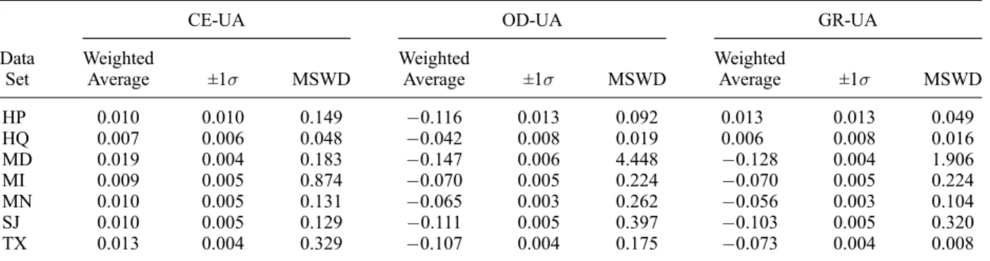
the results are shown in Table 3. All differences in fitted temperature for the CE, OD and GR models are positive, indicating that the UA model yields the coldest NGT estimates. The CE model differ-ences range from 0.215°C for the MI data set, up to 1.368°C for the MD data set. In general, the two models are closest for the coldest records and most disparate for the warmest locations. The OD model is much warmer still, with differences from the UA model ranging from 1.415°C for the HQ data set to 5.353°C for the MD data set. The GR model is similar to the OD model, with the exception of the HP and HQ data sets, where the fitted GR model temperatures are closer to the CE model than the OD model.
[18] To a very good approximation, one can say
that the four different NGT models yield identical temperature records, aside from a constant temper-ature offset. This hypothesis can be tested by examining the variability of the differences as mea-sured by the mean squared weighted deviates (MSWD) of the differences from the error-weighted average, as shown in Table 3. The c2
statistic for the hypothesis of a constant difference can be calculated by multiplying MSWD byn1, wherenis the number of samples in each data set. If MSWD is near to or less than 1, one can conclude that the constant temperature difference hypothesis is supported by the data. In all cases, the MSWD value is less than one and in many cases less than 0.2, indicating a very high degree of coherence between the different models.
2.3. DNe Differences Between Models
[19] A similar analysis was done regarding the
differences of fitted DNe values between the various NGT models and this is shown in Table 4. In all cases, the CE model yields higher DNe values than the UA model and the OD model gives the lowestDNe values. In fact, from Figure 1, the OD model comes the closest to having zero DNe values in some portions of the records. From Table 4, it can be seen that the GR model gives relatively high DNe values (similar to the CE model) for the two Hungarian data sets (HP and HQ), but in all other cases it is much closer to the OD model DNe records. That is, the GR model is very similar to the OD model, but when its optimal POD factor is near 1, the GR model gives records close to the CE model.
[20] The MSWD values are generally very low,
indicating that to a good approximation, there is a constant difference in DNe between the NGT
Figure 1. NGT andDNe records from (a) HP, the P flow system in Great Hungary Basin [Stute and Deak, 1989]; (b) HQ, the Q flow system in Great Hungary Basin [Stute and Deak, 1989]; (c) SJ, the San Juan basin in New Mexico [Stute et al., 1995b]; (d) MI, the Marshall aquifer in Michigan [Ma et al., 2004]; (e) MD, the Aquia aquifer in Maryland [Aeschbach-Hertig et al., 2002a]; (f) MN, the Minqin Basin in China [Edmunds et al., 2006]; and (g) TX, the Carrizo aquifer in Texas [Castro et al., 2007]. Error bars are 1s estimates based upon noble gas volume error estimates using the error propagation techniques outlined byBallentine and Hall[1999].
models. The exceptions to this come from the OD and GR model fits to data from the MD data set. However, almost all of the variability for that data set comes from two samples with extraordinarily high DNe values, i.e., >2, indicating that for those samples, the majority of the Ne is in the excess air component. Therefore, the four different NGT models give similar DNe records, differing only by a nearly constant offset, with the exception of samples with extremely high DNe values.
[21] Despite the existence of systematic differences
between the four models in their fitted NGTs and
DNe values, a remarkable feature of the records shown in Figure 1 and Tables 3 and 4 is that the variations in the fitted parameters are very consis-tent across all of the models. It is clear that although each model handles assignment of the ASW and EA components differently, the underly-ing noble gas concentration data enforce a
remark-able concordance between the methods. The only exceptions appear to be for those samples with relatively high CE error estimates and for samples with extraordinarily high DNe values. This raises the question of whether differences in NGTs and
DNe inferred from noble gas concentrations may in fact be relatively robust and model-independent. In order to test this hypothesis and to see if there are characteristic patterns for how the models fit the data that might be diagnostic for determining whether a particular model is appropriate, we have conducted an extensive statistical test of the models using synthetically generated data.
3. Synthetic Data Tests
[22] A set of artificial NGT data sets were
pro-duced using the UA, CE, OD and GR models as forward models. That is, we assume that each
Table 4. Average Fitted DNe Differencesa Data
Set
CE-UA OD-UA GR-UA
Weighted Average ±1s MSWD Weighted Average ±1s MSWD Weighted Average ±1s MSWD HP 0.010 0.010 0.149 0.116 0.013 0.092 0.013 0.013 0.049 HQ 0.007 0.006 0.048 0.042 0.008 0.019 0.006 0.008 0.016 MD 0.019 0.004 0.183 0.147 0.006 4.448 0.128 0.004 1.906 MI 0.009 0.005 0.874 0.070 0.005 0.224 0.070 0.005 0.224 MN 0.010 0.005 0.131 0.065 0.003 0.262 0.056 0.003 0.104 SJ 0.010 0.005 0.129 0.111 0.005 0.397 0.103 0.005 0.320 TX 0.013 0.004 0.329 0.107 0.004 0.175 0.073 0.004 0.008 a
Weighted averages of the difference between CE, OD and GR modelDNe estimates relative to the UA model for the published paleoclimate records shown in Figure 1. The error estimates are for the average differences and MSWD refers to the mean squared weighted deviates for the three calculated differences. All models are highly correlated as evidenced by the very low MSWD values, with the exception of the MD record, whose elevated OD and GR model MSWDs are caused by two anomalous samples. These samples had high CE model error estimates and therefore they did not significantly affect the CE model MSWD.
Table 3. Average Fitted NGT Differencesa
Data Set CE – UA OD – UA GR – UA Weighted Average (°C) ±1s MSWD Weighted Average (°C) ±1s MSWD Weighted Average (°C) ±1s MSWD HP 0.352 0.240 0.852 3.968 0.212 0.109 0.940 0.221 0.551 HQ 0.390 0.167 0.307 1.415 0.117 0.010 0.503 0.122 0.293 MD 1.368 0.178 0.520 5.353 0.141 0.139 4.855 0.139 0.332 MI 0.215 0.193 0.325 2.379 0.170 0.005 2.379 0.170 0.005 MN 0.600 0.130 0.853 2.558 0.092 0.038 2.384 0.093 0.125 SJ 0.451 0.174 0.446 3.825 0.131 0.032 3.590 0.131 0.024 TX 0.609 0.174 0.751 4.306 0.118 0.021 3.932 0.126 0.432 a
Weighted averages of the difference between CE, OD, and GR model temperature estimates relative to the UA model for the published paleoclimate records shown in Figure 1. The error estimates are for the average differences, and MSWD refers to the mean squared weighted deviates for the three calculated differences. All models are highly correlated as evidenced by the very low MSWD values, in all cases <1 and frequently <0.2. This demonstrates strong coherence between the four different NGT models.
model in turn is perfectly accurate and then pro-duce a suite of perturbed noble gas concentrations assuming a Gaussian distribution of measurement errors. The assumed errors were 1.3%, 1.3%, 1.5% and 2.2% for Ne, Ar, Kr and Xe, respectively, which are the errors quoted byCastro et al.[2007]. All synthetic data sets assumed a recharge altitude of 300 m. For the UA, OD and GR models, the assumed quantity of excess air (parameter A) was set to 0.002 ccSTP/g. For the OD and GR models, a POD factor of 1.1 was assumed and for the GR model a value fort of 3 cm4/3s2/3was assigned (see equation (5) for the definition of thet param-eter). For the CE model, a value for A of 0.01 ccSTP/g was assumed with a fractionation factor Fof 0.7.
[23] For each model, we produced 1000 sets of
noble gas concentrations for true NGT values of 5, 10, 15, 20 and 25°C and thus each model had a total of 5000 sets of synthetic noble gas concen-trations that could then be inverted to derive fitted NGT and DNe values. Solubility values for the noble gases used are those given byBallentine and
given in the auxiliary material in Tables S1– S4 for data produced from the UA, CE, OD and GR models, respectively.1
[24] Because we knew the correct values of the
input parameters, we could measure how well the inversion methods extracted these values from the synthetic data. In all cases, when unperturbed data were inverted, the inversion schemes yielded the correct fitted parameters within floating point precision. For the OD model, a search was made over the entire set of 5000 synthetic samples for an optimal value ofPODand for the GR model, a two-dimensional search was made for its 5000 samples for the best fit combination of PODandt.
3.1. Estimator Bias
[25] The first test was to assess whether each
model’s average fitted NGT and DNe corre-sponded to the known true values. Because of the added Gaussian measurement error, each individu-al fitted vindividu-alue would be expected to differ from the true value, but if the NGT model is an unbiased estimator, the fitted parameters should average to their correct values. The results of this analysis are shown in Figure 2. The UA, OD and GR models all successfully reproduced estimates for NGT and
DNe that averaged to values very close to the true values. However, the CE model, on average, over-estimated temperature by values of 0.22, 0.31, 0.30, 0.39 and 0.37°C for synthetic 5, 10, 15, 20 and 25°C data sets, with an average offset from the true values of 0.32°C. It also overestimated DNe by an overall average value of 0.0031. A similar analysis with a synthetic data set with smaller input error estimates (1% for all gases) was performed and although the CE model performed slightly better, it still systematically overestimated both parameters, indicating that it is a biased estimator for temperature and excess air. It appears that the CE model achieves some of its excellent goodness-of-fit performance by overallocating some of the measured noble gases into the EA component, thereby underestimating the size of the ASW component and leading to a bias toward high fitted temperatures. Cey et al. [2008, 2009] argued that goodness of fit is not a robust indicator of the appropriateness of an NGT model, however, for the CE model, minimizing the goodness of fit param-eter can lead to an overestimation of temperature
Figure 2. Model – true value misfits forTandDNe for 5000 synthetic data reproduced by the UA, CE, OD, and GR models. See section 3 for parameters used to produce the data sets. Each suite of data was fit using the same model that produced the data.
1
Auxiliary materials are available at ftp://ftp.agu.org/apend/gc/ 2009gc002717.
even when it is apparent that the CE model is appropriate to fit synthetic data.
[26] We also investigated whether the OD and GR
models yielded optimalPODand, in the case of the GR model, t values for each individual sets of 1000 synthetic data for the five different assumed groundwater temperatures. In the case of the OD model, the optimal PODvalue was found to be the correct value of 1.10. This reinforces the above finding that the OD model is an unbiased estimator. The case for the GR model, however, is weaker, because the optimal parameters found for POD were 1.10, 1.01, 1.01, 1.11 and 1.12, and the optimal t values were 2.6, 6.0, 5.6, 0.4 and 1.8 for temperatures of 5, 10, 15, 20 and 25°C, respectively. In POD-t space, the minimum c
2
surface is quite flat, which indicates that the POD andtare poorly determined in combination. Given the performance of the GR model over the entire temperature range, with all 5000 samples, it is not possible to say that the model is biased, but care should be taken when using this method. If, for a given suite of data, an incorrectPODis determined, this would have the effect of causing a shift in the NGT values.
[27] A study of the behavior of the CE model
was performed where the F value was assumed to be constant for a synthetic data set, with only A and NGT being determined for each sample, an approach similar to one used by Hall et al. [2005]. The optimal F (i.e., corresponding to the lowestc2value) was the correct value of 0.70 for all five temperatures and the overall average tem-perature estimates were too high by only 0.033°C, an improvement of almost an order of magnitude over the case where F is fit for each individual sample. This indicates that the CE model is not biased when extra information can be used to fix a value ofF, i.e., to use a single value ofFfor a suite of data.
3.2. Patterns of Noble Gas Concentration Misfit
[28] Below, we examine the nature of the average
misfit of the data for the various models to assess whether or not such results might point to features that are susceptible to being detected with real data.
3.2.1. Behavior of the OD Model
[29] Castro et al. [2007] showed that the OD
model improved the fit of Ar and Xe as the POD was gradually raised from a value of 1 (equivalent
to the UA model) to an optimal value of 1.14, which minimized the overall c2 statistic for the data set. A similar analysis is shown in Figure 3 for the synthetic OD model data set, which illustrates that the averagec2value of each fit is minimized at the known correct POD value of 1.1. Note that at low values of POD, model Xe values are systemat-ically too high and Ar values are too low, in good agreement with the plot given by Castro et al. [2007] for the TX data set. The equivalent analysis for the SJ data set [Stute et al., 1995b] is shown in Figure 4 and the correspondence of the general pattern of noble gas misfit with the predictions from the OD model synthetic data is striking. This suggests that the simple addition of a single POD factor that allows for oxygen depletion does a remarkable job of characterizing this data set.
3.2.2. Oxygen Depletion, Altitude Estimation, and the CE Model
[30] Another feature that was investigated was
whether the allowance for oxygen depletion in soil gas could be added to the CE model’s mechanism for handling the EA component, with the effect of possibly improving the CE model. Unfortunately, whenever an attempt was made to derive an optimal POD factor from a synthetic data set, the POD value that gave the lowest c2 statistic was invariably too low. In fact, when trying to deduce an optimal POD factor for the standard CE model synthetic data (i.e.,POD= 1), the best goodness of fit occurred forPOD< 1, i.e., equivalent to oxygen enrichment. From equation (4) above, POD values below 1 are equivalent to setting a higher altitude than the actual recharge altitude assuming standard air composition. Ballentine and Hall[1999] inves-tigated whether a suite of NGT data could be used to deduce the actual recharge altitude, when it is unknown, by finding the best goodness of fit for the suite of data. A similar style of analysis was done byManning and Solomon[2003, 2005] using the UA model. Given the fact that the OD model has been shown to be an unbiased estimator for both temperature and DNe, one should expect that the UA model is an unbiased estimator for altitude because the pressure correction factor for altitude is mathematically equivalent to using aPODfactor for oxygen depletion. However, given that when aPOD factor is added to the CE model, an optimal fit is obtained with an incorrect POD factor, it might be expected that the CE model would not be appro-priate for estimating the altitude of recharge.
[31] We show this kind of analysis for the CE
model data in Figure 5, where the average CE modelc2value per sample is plotted as a function of the assumed recharge altitude as calculated for the 5000 CE model generated synthetic noble gas data values. We know that the correct recharge altitude for the synthetic data is 300 m, but it can clearly be seen that the best fits occur when one assumes an altitude of >1000 m. This illustrates the strong tendency for the CE model, in the presence of measurement error, to improve upon the fit by artificially increasing the EA component at the expense of the ASW component. The combination of the A andF factors within the CE model gives the method greater freedom when the EA
compo-nent is large and this could explain why the CE model tends to overestimate both DNe and NGT. In any case, it is clear that studies attempting to deduce an aquifer’s recharge altitude from ground-water noble gas data should not use the CE model for the estimation, as it will tend to give an altitude value that is biased high.
3.2.3. Cross Fitting Models With Synthetic Data
[32] Figure 6 shows the results of fitting one
model’s synthetic data using another model, to see how well a model can cope with nonideal data, i.e., where their underlying assumptions do not
Figure 3. Averagec2per sample and average model – data misfit (in units of measurements) for each noble gas as a function ofPODusing the OD method for synthetic data produced by the OD model. The correct value ofPOD
match the true forward model parameters. The NGT misfits are shown in Figure 6a and it can be seen that the UA model slightly underestimates temperature for CE model data, but it is much more inaccurate for OD and GR model data, under-estimating temperature by 3°C. Surprisingly, although the CE model includes the UA model for F = 0, it still overestimates temperature for UA model data in a similar manner to its over-estimation of CE model data. The CE model does better than the UA model with OD and GR data, with an average NGT that is about 2°C too low. The OD model slightly overestimates UA and GR model data and it overestimates CE model data by
2°C. The GR model is the most successful in estimating NGTs, with its worst misfit being a
0.6°C overestimation for CE model data.
[33] Despite these systematic offsets in temperature
estimates, there is remarkable agreement for all models over temperature differences within a data set. Figure 6b shows the average difference be-tween the 25°C NGT fits and those for 5°C estimates. Ideally, the temperature difference should be 20°C and all models are within 1°C of being correct, despite this being an extreme tem-perature range that is not likely to be seen within most paleoclimate records. In this regard, the UA model is the worst performer and the OD and GR models are the best, but all models would tend to give nearly identical records of temperature vari-ability. This confirms the pattern seen with pub-lished data as shown in Figure 1. Figure 6c shows
DNe misfits for the four models and it illustrates that although the UA and CE models fit each
Figure 4. Averagec2per sample and average model – data misfit (in units of measurements) for each noble gas as a function ofPODusing the OD method for the SJ data set [Stute and Deak, 1989]. Note the similarity to the synthetic
other’s data relatively well, they both overestimate
DNe for the OD and GR models. The OD model underestimates DNe for CE model data and again the GR model seems to have the best overall performance with only a small underestimation of
DNe for CE model data.
3.2.4. Patterns of Noble Gas Concentration Misfit
[34] Figure 7 shows details on how well each
model fits the individual noble gases. The misfits are average model value minus data and they are scaled in terms of the noble gas measurement error estimate (s). Ideally, each noble gas should be accurately modeled, with an average value close to zero. When there are systematic offsets, this indicates that the model is having difficulty cor-rectly assigning the ASW and EA components. The UA model has the most difficulty in fitting other model’s data (note the larger scale of the UA fitting pattern) and the plot demonstrates a diag-nostic pattern. When there is an extra temperature-dependent ASW component, either from dissolution at elevated pressure with trapped air bubbles (CE model) or due to elevated noble gas pressure because of oxygen depletion (OD and GR models), the UA model significantly underestimates Ar and overestimates Xe concentrations, while both Ne and Kr concentrations tend to be fit reasonably well. The CE model results are in many ways the
mirror image of the UA model fits in that the CE model tends to overestimate Ar while underesti-mating Xe, even for data generated with the CE model or the UA model, which is a subset of the CE model. A significant underestimation for Kr concentrations appears to be unique to the CE model. In contrast, the OD and GR models fit most models relatively well, but they have the greatest difficulty with CE model data, exhibiting a tendency to overestimate Kr concentration.
[35] Finally, we show the pattern of noble gas
misfits for all of the NGT paleoclimate records illustrated in Figure 1. Figure 8 shows these patterns and it is clear that the CE model does an excellent job of fitting data for the MD and MN studies. However, the CE model tends to have significant negative Kr anomalies (i.e., underesti-mating Kr) for the other data sets. With the exception of the MI data set, all other records demonstrate the characteristic UA misfit pattern at Ar and Xe, which tends to indicate an ASW component that cannot be correctly accounted for using the UA model. The MI record causes diffi-culties for all models, but this may be caused by the extremely low NGT values that are derived from this data set (i.e., <5°C) and therefore these data are at the extreme end of the range of Kr and Xe concentrations expected for noble gases in groundwater. The OD and GR models perform very well for the HP, HQ, SJ, MN and TX records
Figure 5. Averagec2for CE model fit of synthetic data produced by the CE model. The true recharge altitude is 300 m, but the goodness of fit keeps improving at much greater altitudes.
despite having far fewer fitted parameters than those for the CE model. Given their relative simplicity and the fact that they are unbiased estimators for temperature andDNe, these models are probably the most appropriate ones for use with the HP, HQ, SJ, MN and TX data sets. In the case of the TX data set, there is independent evidence from ground temperature in the recharge area that suggests that the OD and GR models are signifi-cantly more accurate than the UA and CE models [Castro et al., 2007].
[36] In our use of the OD and GR models, we have
assumed that to a reasonable approximation, the POD and/or t parameters are a constant for an entire data set. This is known to be true for the synthetic data that was produced, but it is entirely possible that these parameters vary with time for real data. The temptation exists to try to fit at least one of these parameters to individual noble gas sample measurements, but this leads to numerical instabilities and a significant growth in temperature
Figure 6. (a) Average model – true misfits of temperature for synthetic data. The models that produced the synthetic data are encoded as blue for UA model, red for CE model, orange for OD model, and green for GR model. (b) Average difference between temperature fits for 25°C minus 5°C synthetic data, with the true difference being 20°C. Note that all models have differences that are within 1°C of the correct value despite fitting data produced by another model. (c) Average model – trueDNe misfits for synthetic data.
error estimates. This is similar to what happened to CE model fits of data from the MI and TX records.
4. Conclusions
[37] By applying a wide range of NGT models
(UA, CE, OD, and GR) to a series of groundwater noble gas concentration data sets, we show that although there are significant differences between models, both for estimated temperature and excess air, nevertheless the amount of variation in these estimated parameters is remarkably consistent, suggesting that estimates of climate change history derived from variations of temperature and excess
air are robust. This was theoretically confirmed using 5000 synthetic data produced using one model but fit with another. Even with a 20°C change in assumed recharge temperature, an incor-rect model will display a corincor-rect temperature dif-ference within about 1°C. It is expected that smaller temperature changes will be even more accurate. It should be noted, however, that this consistency for estimating temperature changes only holds true if the same NGT model is used throughout the analysis of an entire data set. If multiple models are used, the significant offsets between models may introduce apparent tempera-ture variations that are artifacts of the choice of NGT inversion method.
Figure 7. Average model – data misfits for each noble gas for synthetic data, in units of measurement errors. The models that produced the synthetic data are encoded as blue for UA model, red for CE model, orange for OD model, and green for GR model. Note expanded scales for the OD and GR models.
[38] To assess which NGT model might produce
the most accurate results, we first investigated whether all four models were unbiased paleocli-matic estimators. The UA, OD and GR models were shown to be unbiased estimators of temper-ature and excess air when fitting synthetic data that those models produced. However, the CE model has a definite tendency to overestimate both tem-perature and excess air. The model achieves some of its excellent goodness-of-fit performance by inflating the excess air component, which gives the model more flexibility in fitting data errors. Related to this problem is the fact that the CE model will tend to overestimate the recharge alti-tude of an aquifer and it should not be used for this purpose. By preferring an erroneously high alti-tude, the CE model is, on average, reducing the ASW component below its true value and
increas-ing a fractionated excess air component to com-pensate. The CE model should be used with care as it is not an unbiased estimator and its large number of fitted parameters sometimes makes the system close to being underdetermined. Achieving maxi-mum likelihood by means of minimizing a c2
statistic is no guarantee of accuracy when the underlying method is not an unbiased estimator. Alternatively, given that the CE model is not a biased estimator when using a fixed F factor, it should be possible to use the CE model for recharge altitude estimation, or even in combina-tion with a PODfactor, provided thatFis not fit to individual samples.
[39] Additionally, we examined diagnostic means
to judge which model may be more suitable for a particular set of data based upon the noble gas
Figure 8. Average model – data noble gas misfits for the noble gas data sets illustrated in Figure 1. Units are measurement errors. Fitting models used are color coded as follows: blue, UA; red, CE; orange, OD; and green, GR. Data set misfit patterns shown are (a) HP, (b) HQ, (c) SJ, (d) MI, (e) MD, (f) MN, and (g) TX. See section 2 for references.
models produce synthetic data that causes a diag-nostic misfit pattern when inverted by the UA model: that is, the inversion underestimates Ar and overestimates Xe. This pattern is seen repeat-edly in real data sets and suggests that some of the ASW component is modified by elevated pres-sures, either in trapped air bubbles (CE model) or due to oxygen depletion (OD and GR models). The GR model is quite versatile, being able to ade-quately fit all the other models. However, if there is significant excess air and if the fittedt is large, the GR model would predict significant fractionation of Ne and Ar isotope ratios and if the predicted ratios are incompatible with data, either the OD or CE model should be used.
Acknowledgments
[40] The authors thank J. A. Tarduno and D. R. Hilton for the editorial handling of this manuscript as well as reviewers C. J. Ballentine and B. D. Cey for their thoughtful and constructive comments. Financial support by the National Science Foun-dation CAREER award EAR-0545071 is greatly appreciated.
References
Aeschbach-Hertig, W., F. Peeters, U. Beyerle, and R. Kipfer (1999), Interpretation of dissolved atmospheric noble gases in natural waters, Water Resour. Res., 35(9), 2779 – 2792, doi:10.1029/1999WR900130.
Aeschbach-Hertig, W., F. Peeters, U. Beyerle, and R. Kipfer (2000), Paleotemperature reconstruction from noble gases in ground water taking into account equilibration with entrapped air, Nature, 405, 1040 – 1044, doi:10.1038/ 35016542.
Aeschbach-Hertig, W., M. Stute, J. F. Clark, R. F. Reuter, and P. Schlosser (2002a), A paleotemperature record derived from dissolved noble gases in groundwater of the Aquia Aquifer (Maryland, USA), Geochim. Cosmochim. Acta, 66(5), 797 – 817, doi:10.1016/S0016-7037(01)00804-3. Aeschbach-Hertig, W., U. Beyerle, J. Holocher, F. Peeters, and
R. Kipfer (2002b), Excess air in groundwater as a potential indicator of past environmental changes, inStudy of Envir-onmental Change Using Isotope Techniques, pp. 174 – 183, Int. At. Energy Agency, Vienna.
Aeschbach-Hertig, W., H. El-Gamal, M. Wieser, and L. Palcsu (2008), Modeling excess air and degassing in groundwater by equilibrium partitioning with a gas phase,Water Resour. Res.,44, W08449, doi:10.1029/2007WR006454.
Ballentine, C. J., and C. M. Hall (1999), Determining paleo-temperature and other variables by using an error-weighted nonlinear inversion of noble gas concentrations in water, Geochim. Cosmochim. Acta, 63(16), 2315 – 2336, doi:10.1016/S0016-7037(99)00131-3.
Brennwald, M. S., M. Hofer, F. Peeters, W. Aeschbach-Hertig, K. Strassmann, R. Kipfer, and D. M. Imboden (2003), Ana-lysis of dissolved noble gases in the porewater of lacustrine sediments,Limnol. Oceanogr. Methods,1, 51 – 62.
Brennwald, M. S., R. Kipfer, and D. M. Imboden (2005), Release of gas bubbles from lake sediment traced by noble
Lett.,235, 31 – 44, doi:10.1016/j.epsl.2005.03.004. Castro, M. C., C. M. Hall, D. Patriarche, P. Goblet, and B. R.
Ellis (2007), A new noble gas paleoclimate record in Texas—Basic assumptions revisited,Earth Planet. Sci. Lett., 257(1 – 2), 170 – 187, doi:10.1016/j.epsl.2007.02.030. Cey, B. D., G. B. Hudson, J. Moran, and B. R. Scanlon (2008),
Impact of artificial recharge on dissolved noble gases in groundwater in California, Environ. Sci. Technol., 42, 1017 – 1023, doi:10.1021/es0706044.
Cey, B. D., G. Bryant, G. B. Hudson, J. E. Moran, and B. R. Scanlon (2009), Evaluation of noble gas recharge tempera-tures in a shallow unconfined aquifer, Ground Water, 47, 646 – 659, doi:10.1111/j.1745-6584.2009.00562.x.
Edmunds, W. M., J. Ma, W. Aeschbach-Hertig, R. Kipfer, and D. P. F. Darbyshire (2006), Ground water recharge history and hydrogeochemical evolution in the Minqin Basin, north west China, Appl. Geochem., 21(12), 2148 – 2170, doi:10.1016/j.apgeochem.2006.07.016.
Hall, C. M., M. C. Castro, K. C. Lohmann, and L. Ma (2005), Noble gases and stable isotopes in a shallow aquifer in south-ern Michigan: Implications for noble gas paleotemperature reconstructions for cool climates, Geophys. Res. Lett., 32, L18404, doi:10.1029/2005GL023582.
Heaton, T. H. E., and J. C. Vogel (1981), ‘‘Excess air’’ in groundwater, J. Hydrol., 50(1 – 4), 201 – 216, doi:10.1016/ 0022-1694(81)90070-6.
Ma, L., M. C. Castro, and C. M. Hall (2004), A late Pleisto-cene-Holocene noble gas paleotemperature record in south-ern Michigan,Geophys. Res. Lett.,31, L23204, doi:10.1029/ 2004GL021766.
Manning, A. H., and D. K. Solomon (2003), Using noble gases to investigate mountain-front recharge,J. Hydrol.,275(3 – 4), 194 – 207, doi:10.1016/S0022-1694(03)00043-X.
Manning, A. H., and D. K. Solomon (2005), An integrated environmental tracer approach to characterizing groundwater circulation in a mountain block, Water Resour. Res., 41, W12412, doi:10.1029/2005WR004178.
Mazor, E. (1972), Paleotemperatures and other hydrological parameters deduced from noble gases dissolved in ground-waters: Jordan Rift Valley, Israel, Geochim. Cosmochim. Acta, 36(12), 1321 – 1336, doi:10.1016/0016-7037(72) 90065-8.
Mercury, L., D. L. Pinti, and H. Zeyen (2004), The effect of the negative pressure of capillary water on atmospheric noble gas solubility in ground water and paleotemperature recon-struction, Earth Planet. Sci. Lett., 223(1 – 2), 147 – 161, doi:10.1016/j.epsl.2004.04.019.
Peeters, F., U. Beyerle, W. Aeschbach-Hertig, J. Holcher, M. Brennwald, and R. Kipfer (2003), Improving noble gas based paleoclimate reconstruction and groundwater dating using20Ne/22Ne ratios, Geochim. Cosmochim. Acta, 67(4), 587 – 600, doi:10.1016/S0016-7037(02)00969-9.
Saar, M. O., M. C. Castro, C. M. Hall, M. Manga, and T. P. Rose (2005), Quantifying magmatic, crustal, and atmo-spheric helium contributions to volcanic aquifers using all stable noble gases: Implications for magmatism and ground-water flow, Geochem. Geophys. Geosyst., 6, Q03008, doi:10.1029/2004GC000828.
Stute, M., and J. Deak (1989), Environmental isotope study (14C,13C,18O, D, noble gases) on deep groundwater circula-tion systems in Hungary with reference to paleoclimate, Radiocarbon,31(3), 902 – 918.
Stute, M., and P. Schlosser (1993), Principles and applica-tions of the Noble gas paleothermometer, in Climate Change in Continental Isotopic Records,Geophys. Monogr.
Ser., vol. 78, edited by P. K. Smart et al., pp. 89 – 100, AGU, Washington, D. C.
Stute, M., P. Schlosser, J. F. Clark, and W. S. Broecker (1992), Paleotemperatures in the Southwestern United States derived from noble gases in ground water, Science, 256(5059), 1000 – 1001.
Stute, M., M. Forster, H. Frischkorn, A. Serjo, J. F. Clark, P. Schlosser, W. S. Broeker, and G. Bonani (1995a), Cooling of tropical Brazil (5°C) during the last glacial max-imum,Science,269(5222), 379 – 383, doi:10.1126/science. 269.5222.379.
Stute, M., J. F. Clark, P. Schlosser, W. S. Broecker, and G. Bonani (1995b), A 30,000 yr continental paleotem-perature record derived from noble gases dissolved in groundwater from the San Juan Basin, New Mexico, Quat. Res., 43(2), 209 – 220, doi:10.1006/qres.1995.1021. Sun, T., C. M. Hall, M. C. Castro, K. C. Lohmann, and P. Goblet (2008), Excess air in the noble gas groundwater paleothermometer: A new model based on diffusion in the gas phase, Geophys. Res. Lett., 35, L19401, doi:10.1029/2008GL035018.
Wilson, G. B., and G. W. McNeill (1997), Noble gas recharge temperatures and the excess air component,Appl. Geochem., 12(6), 747 – 762, doi:10.1016/S0883-2927(97)00035-8.
![Figure 1. NGT and DNe records from (a) HP, the P flow system in Great Hungary Basin [Stute and Deak, 1989];](https://thumb-us.123doks.com/thumbv2/123dok_us/9351594.2813583/7.918.114.803.137.987/figure-ngt-records-great-hungary-basin-stute-deak.webp)