Computer Science and Artificial Intelligence Laboratory
Technical Report
m a s s a c h u s e t t s i n s t i t u t e o f t e c h n o l o g y, c a m b r i d g e , m a 0 213 9 u s a — w w w. c s a i l . m i t . e d u
MIT-CSAIL-TR-2017-011
June 9, 2017
An Efficient Fill Estimation Algorithm for
Sparse Matrices and Tensors in Blocked Formats
Peter Ahrens, Nicholas Schiefer, and Helen Xu
An Efficient Fill Estimation Algorithm for Sparse Matrices
and Tensors in Blocked Formats
Peter Ahrens
[email protected]
Nicholas Schiefer
[email protected]
[email protected]
Helen Xu
AbstractTensors, which are the linear-algebraic extensions of matrices in arbitrary dimensions, have numerous applications to data processing tasks in computer science and computational science. Many tensors used in diverse application domains are sparse, typically containing more than 90% zero entries. Efficient computation with sparse tensors hinges on algorithms that can leverage the sparsity to do less work, but the irregular locations of the nonzero entries pose significant challenges to performance engineers. Many tensor operations such as tensor-vector multiplications can be sped up substantially by breaking the tensor into equally sized blocks (only storing blocks which contain nonzeros) and performing operations in each block using carefully tuned code. However, selecting the best block size from among many possibilities is computationally challenging.
Previously, Vuduc et al. defined the fill of a sparse tensor to be the number of stored
entries in the blocked format divided by the number of nonzero entries, and showed how the fill can be used as part of an effective, efficient heuristic for evaluating the quality of a particular blocking scheme [1, 2]. In particular, they showed that if the fill could be computed exactly, then the measured performance of their sparse matrix-vector multiply was within 5% of the optimal setting. However, they gave no theoretical accuracy bounds for their method for estimating the fill, and it is vulnerable to several classes of adversarial examples.
In this paper, we present a sampling-based method for finding a (1 +ε)-approximation to the fill of an order N tensor for all block sizes less thanB, with probability at least 1−δ, using O(NBNlog(B/δ)/ε2) samples for each block size. We introduce an efficient routine
to sample for all BN block sizes at once in O(NBN) time. We extend our concentration
bounds to a more efficient bound based on sampling without replacement, using the recent Hoeffding-Serfling inequality [3]. We then implement1our algorithm and evaluate it on sparse matrices from the University of Florida collection and compare our scheme to that of Vuduc, as implemented in the Optimized Sparse Kernel Interface (OSKI) library, and a brute-force method for obtaining the ground truth. We find that our algorithm provides faster estimates of the fill at all accuracy levels, providing evidence that this is both a theoretical and practical improvement.
1 Introduction
Tensors are multi-dimensional generalizations of matrices. They have important applications in the physical and computational sciences, ranging from machine learning to computational chemistry. Many tensors used in diverse application domains are sparse, typically containing more than 90% zero entries. Most fundamental linear algebraic operations on tensors, such as tensor-vector multiplications, run in time proportional to the number of elements in the tensors. Sparse tensors provide an opportunity to write algorithms and data structures with complexity proportional to the number of nonzero entries, with substantial increases in performance. However, the increased complexity of data structures that can describe the irregular locations of nonzeros in these tensors poses a significant challenge to algorithm designers and performance engineers.
1.1 The problem of selecting a block size 1 INTRODUCTION
These challenges will only grow as architectures become increasingly specialized. In order to write the most efficient sparse tensor code, the programmer must take into account both the target architecture and the relevant structural properties of the nonzeros of the sparse tensor. Writing custom code for each processor requires extensive engineering effort. Additionally, the
structure of nonzeros in a sparse tensor is usually known only at runtime. As a result,autotuning
(automatically generating customized code) has become a necessary part of writing efficient code for operations on sparse tensors.
Sparse Tensor Representations. Previous efforts in autotuning for sparse tensors focus on sparse matrices, which see the broadest application. The diverse space of operations and nonzero patterns of sparse matrices have led to the development of a wide variety of sparse matrix formats that allow programmers to more efficiently operate on the matrices. Perhaps the most popular
such format is the Compressed Sparse Row (CSR) [4]. Like most sparse matrix formats, CSR
stores only the locations and values of the nonzero entries of the matrix; the specific details of the format are not relevant to the present exposition and are omitted. Note that the results in this paper apply to any sparse matrix format which can be generalized to include a block structure.
To decrease the complexity of storing the locations of individual nonzeros, performance
engi-neers have developed a variant of CSR called Blocked Compressed Sparse Row (BCSR) [5]. In
BCSR, anm×nmatrix is partitioned intom/r×n/csubmatrices, where each submatrix is of size
r×c. The submatrices are called blocks, and are stored in a dense format, with zeros represented
explicitly. Only blocks which contain nonzeros are stored, and the locations of the stored blocks are recorded using CSR format.
The key advantage of the BCSR format (and blocked formats in general) is the reduced com-plexity of operations on the “dense” part of the matrices. For example, consider the common operation of a matrix-vector multiplication. If a matrix has a natural block structure, then the blocked matrix can be multiplied by a blocked vector using standard CSR methods, but the individual blocks can be multiplied using a small, fixed-size, dense matrix-vector multiply. Per-formance engineers have experience in writing efficient code for small dense linear algebra kernels. The programmer and compiler can utilize standard techniques like loop unrolling, register and cache blocking, and instruction-level parallelism.
Matrices with a natural block structure appear in numerous applications, such as matrices produced by finite element methods. The BCSR format can be extended naturally to support higher-dimensional tensors as well [6, 7, 8].
Preliminaries. Throughout this paper, we will discuss N-dimensional tensors in a particular
orthogonal basis. That is, tensors areN-dimensional arrays of elements over some fieldF, usually
the real or complex numbers. We denote tensors by capital script lettersAand vectors by lowercase
boldface lettersa.
The element of an orderN tensorAindexed by (i1, i2, . . . , iN) is denotedA[i1, i2, ..., iN]. For
compactness of notation, we sometimes specify an index into a tensor as aN-component vector
i= (i1, i2, . . . , iN). If we wish to represent the integer rangei, i+1, ..., i0, we use the syntaxi→i0.
If we wish to represent the range of indices between two vectors, we use the syntaxi→i0, meaning
i1 →i01, ..., iN →i0N. Subtensors are formed when we fix a subset of indices. We use a colon to
indicate all elements along a particular dimension. Thus, the middle n/2 columns of a matrix
A ∈Fn×n would be writtenA[:, n/4→3n/4].
The number of nonzero entries in a A is denoted k(A). When we compare a vector to a
scalar, we mean to compare each entry of the vector pointwise. For notational convenience, we
occasionally redefine the starting index of a tensor. Thus,A ∈ FI→I0
is an (I0
1−I1+ 1)×...×
(I0
N −IN+ 1) tensor whose smallest index isIand largest index isI0.
1.1 The problem of selecting a block size
Since the performance of blocked sparse tensor operations depends on the block size, we must find some block size that gives good—and ideally the best—performance on the matrix. If we
1.1 The problem of selecting a block size 1 INTRODUCTION
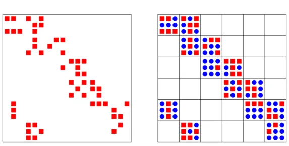
Figure 1.1 – A sparse matrix before blocking (left) and an example of a blocked sparse matrix (right). The squares denote nonzero elements and circles are explicit zeros that are introduced due
to the blocking scheme. In this example, the blocking scheme is defined by b = (3,3) resulting
inkb = 13. The number of nonzero elements k(A) = 52, so we can compute the fill as follows:
fb= (3×3×13)/52 = 2.25.
set the block size too small, then we must store the locations of more blocks, and we waste time processing the block locations. If we set the block size too large, then the blocks will be filled with too many zeros, and we waste time computing unnecessary dense matrix operations.
Definition 1.1. Ablocking scheme bof a tensorA ∈FI1×I2×···×In is parameterized by a vector
b = (b1, b2, . . . , bN) of block sizes. The blocking scheme induced by b is a partition of A into
N-dimensional subtensors with bi entries along the ith dimension. Thus, a nonzero at location i
would be stored at the block index
i1 b1 , i2 b2 , ..., iN bN .
We present an example of a blocking scheme in a sparse matrix in Figure 1.1. Blocked formats fill in the empty slots of nonempty blocks with explicit zeroes and do not fill in empty blocks.
When manipulating a sparse tensorA, we want to find a blocking scheme that includes all of the
nonzero entries ofAin few blocks. We are therefore interested in the number of blocks containing
a nonzero under the blocking schemeb, which we denotekb(A). Notice that k1(A) =k(A), since
tilingAinto unit-size blocks will have exactly one non-empty block for every nonzero.
Intuitively, a blocking scheme is good if it packs all of the nonzeros into a small number of
non-empty blocks. We define thefill, which captures this notion of blocking scheme quality:
Definition 1.2 (Vuduc et al. [2]). Thefill of a tensorA with respect to a particular blocking
schemebis the ratio
fb(A) =b1b2· · ·k(bAn)kb(A).
That is, the fill is the ratio of the number of entries in nonempty blocks in the blocking schemeb
ofAto the number of nonzeros inA. Where it is clear what tensor we are referring to, we often
write the fill asfb.
In their seminal work, Vuduc et al. demonstrate that the fill can be used as an effective heuristic
for predicting the performance of a particular block size on a sparse matrixA. They showed that
when the fill was known exactly, performance of the resulting blocking scheme was optimal or near-optimal (within 5%) on all of the platforms that they tested [2]. Once per machine, we compute
1.2 Our contributions 1 INTRODUCTION
a profile of how the machine performs for a particular block size. Let Pb be the performance of
the machine (in MFLOP/s) on a dense matrix stored with blocking scheme b. We can think of
Pb as a measure of how efficiently we can process nonzeros when nonzeros are stored in blocks of
sizeb. We can estimate the performance of the machine on the BCSR format ofAasPb/fb(A). Unfortunately, the fill of a tensor with respect to a blocking scheme can vary substantially depending on the tensor’s structure. The blocking scheme that minimizes the fill of a tensor can be found by searching over all possible blocking schemes and computing the number of nonempty blocks for each. However, it is computationally intractable in practice to calculate the fill exactly, since we would spend far more time estimating the fill to find the optimal blocking scheme than we would performing the tensor operations directly [9, 2].
In practice, we care only about block sizes that are small enough to fit in most L1 caches, which is typically at most 12 entries along both dimensions for matrices [9]. Furthermore, the cost of calculating the fill rivals the performance benefits obtained from blocking. Thus, our problem is to quickly compute an approximation to the fill with reasonable accuracy:
Problem 1.1 (Fill approximation problem). Given a tensor A and a maximum block size B,
compute a (randomized) approximationFb(A) such that
(1−ε)fb(A)≤Fb(A)≤(1 +ε)fb(A)
for all block sizes b≤ B, with probability at least 1−δ. Equivalently, we want to compute a
random variableFb(A) such that
Pr max b≤B |fb−Fb| fb > ε ≤δ .
Previously, Vuduc et al. gave sampling methods for estimating the fill of a sparse matrix, but did not give any theoretical analysis of the accuracy of their method. Furthermore, their method takes as long as 1 to 10 times the time it takes to perform a sparse matrix-vector multiplication on the same matrix [9].
1.2 Our contributions
We describe the first algorithm which solves the fill approximation problem with provable guar-antees, and demonstrate that it is faster and more accurate on a suite of sparse matrices than the state-of-the-art algorithm due to Vuduc [2]. At a high level, our algorithm repeatedly samples a nonzero entry in the tensor, then computes the number of nonzero elements in the block of that entry, for all possible blocking schemes. For each blocking scheme, it then averages the reciprocal of this count over all sampled indices. We provide a more detailed description of this sampling algorithm in Section 3. We show that this is an unbiased estimator for the fill of the tensor, and give tight concentration bounds.
More formally, suppose that our algorithm is given a maximum block size B and a sparse
tensor A. Our algorithm repeatedly samples a location i from a tensor A. For each blocking
scheme b ≤ B, it computes the number zb(i) of nonzero entries in the block that i appears in
under the blocking schemeb. After drawing a total ofS samples i1,i2, . . . ,iS, it computes the
averages Fb:= b1b2S· · ·bN S X j=1 1 zb(ij) for allb≤B.
Our algorithm extends the concept of fill from sparse matrices to general sparse tensors in
a natural way. We also contribute a fast, tightly optimized method for computing zb(i) for all
1.2 Our contributions 1 INTRODUCTION
1.2.1 Theoretical contributions
We provide the first rigorous analysis of an algorithm for approximating the fill of anN-dimensional
tensor under a particular blocking scheme. We provide a full analysis of our sampling method in Section 4.
First, we show that our sampling-based algorithm is indeed an unbiased estimator for the fillfb
(with expectation equal to the fill):
Theorem 1.1. For any blocking scheme b, the random variable Fb is an unbiased estimator for
the fill: that is,E[Fb] =fb(A).
An unbiased estimator is useful only if it has reasonable concentration about its mean. Prior
work on fill estimation gaveno theoretical analysis of the concentration of the estimator, in part
because the heuristic is not conducive to theoretical analysis. In fact, prior methods suffer from vastly worse performance on certain adversarial examples, as we show experimentally in Section 5.
In contrast, we give two concentration bounds for Fb, showing that our algorithm solves the
fill approximation problem so long as we use enough samples. If we sample the nonzeros with replacement, an analysis based on Hoeffding’s inequality gives that:
Theorem 1.2. If we sample at least NBN
2ε2 log 2δB
samples with replacement, then Pr max b≤B |fb−Fb| fb ≤ε ≥1−δ .
Notice that for constantδ, this bound is independent of the number of nonzerosk(A), whereas
the algorithm introduced by Vuduc et al. depends linearly upon the number of nonzeros [2].
Because it runs in constant time with respect to the number of nonzeros, the bound onS could
(and does, for realistic settings ofε and δ) exceed the number of nonzeros. This is fundamental
to bounds based on Hoeffding’s inequality, and methods based on sampling-with-replacement in general.
To avoid this issue, we consider the case where we sample without replacement. This analysis
is more involved, since the sampled locations are no longer independent and so we cannot use Hoeffding’s inequality. Instead, we use the recent Hoeffding-Serfling inequality, due to Bardenet and Maillard, obtaining a strictly tighter bound, which is also at most the number of nonzeros [3]. Theorem 1.3. Let T =NBN 2ε2 log 2δB . If S≥ T−T/k(A) + p (T−T/k(A))2+ 4T(1 +T/k(A)) 2 + 2T/k(A) , then Pr max b≤B |fb−Fb| fb ≥ε ≤δ . 1.2.2 Experimental contributions
We implemented2 the sampling algorithm described in Section 3 for sparse CSR matrices in C
and compared it against the existing algorithm for fill estimation proposed by Vuduc et al. [9] using the same test matrices. We also examine the performance on pathological inputs for each algorithm. We show that our algorithm approximates the fill more accurately and quickly than the existing method and present our findings in 5.
Finally, we note that estimating the fill can be an important part of any sparse data structure which uses blocking, not just BCSR. In fact, any sparse data structure can be adapted to a blocked regime by grouping a tensor into blocks and simply treating nonzero blocks as nonzeros of some sparse tensor.
2 RELATED WORK
2 Related Work
Fill estimation is an important intermediate step in autotuning blocked sparse matrix compu-tations [10, 1, 11, 12, 13]. Previous work also includes autotuning for matrix compucompu-tations on GPUs [14] and performance tuning for sparse matrix kernels [15, 16].
To our knowledge, there are no theoretical guarantees on the accuracy of existing algorithms for fill estimation in matrices. [9] provides an empirical study.
2.1 OSKI Heuristic for fill estimation
We first describe the existing heuristic for fill estimation. Since the algorithm is implemented in
the Optimized Sparse Kernel Interface (OSKI) library, we will refer to it asOSKI[2]. OSKIsamples
from the nonzero structure using some user-chosen parameterσ∈[0,1] that adjusts the runtime
and accuracy of the algorithm.
Most of the work in OSKI is accomplished in the EvaluateRows subroutine. LetB be the
maximum number of rows or columns in a block — that is, the maximum block size is B×B
(recall that for matrices, a typical setting ofB is 12). EvaluateRows computes an estimate of
the fill for a fixedrand all 1≤c≤B. Let the input matrixAhave dimensionsm×n. We define
thei-thblock row to be the rowsirthrough (i+ 1)r−1 (A[ir→(i+ 1)r−1,:]). EvaluateRows
exactly computes the number of nonzero blocks in an expected fractionσof the block rows. OSKI
works by callingEvaluateRowsonce for each row size 1≤r≤B.
EvaluateRows evaluates an expected fraction σof block rows by evaluating each one with
probability σ. For each block row thatEvaluateRows chooses to evaluate, it usesB arrays of
lengthn(this construct is referred to asblocks visited) to store the number of nonzeros seen so
far in each block as it iterates over the nonzeros ofA[ir→(i+1)r−1,:] in row-major order. Each
time a nonzero is seen in a previously unvisited block of sizer×c, the estimate of the number of
blocks of sizer×c(stored in an array as nnz visited[c]) is incremented.
For each blocking scheme (r, c), the fill estimate is defined by
Fr,c(A, σ) =rc(nnz visitedσk(A) r[c])
We provide pseudocode for EvaluateRowsin Algorithm 2.1. The function takes as input a
tensor A, maximum block dimensionB, evaluation probability σ, and a fixed row dimensionr.
The algorithm estimates the fill for all blocking schemes with row dimension r. To compute fill
estimates for all blocking schemes, we call the function once for each possible row dimensionr.
Algorithm 2.1. 1: functionEvaluateRows(A,B,σ, r) 2: 3: blocks visitedc ∈Nn∀1≤c≤B 4: nnz visited∈NB 5: blocks visitedc ←0∀1≤c≤B 6: nnz visited←0 7: fori∈1→m/r do
8: Flip a coin with heads probabilityσ.
9: if heads then
10: fornonzero column indices j inA[s, t]∈ A[ir→(i+ 1)r−1,:] do
11: forc∈1→B do
12: nnz visitedr←nnz visitedr+ 1
13: blocks visitedc[bj/cc]←blocks visitedc[bj/cc] + 1
14: if blocks visitedc[bj/cc]←1then
15: nnz visited[c]←nnz visited[c] + 1
3 THE ALGORITHM
Theorem 2.1. OSKI takes time Ω(σB2k(A))in expectation.
Proof. First, notice that the algorithmEvaluateRowstakes Ω(σBk(A)) time in expectation.
Since each block row is evaluated with probability σ, each nonzero in the matrix is
evalu-ated with probability σand since the algorithm performs at leastB operations for each nonzero
evaluated, the algorithm takes Ω(σBk(A)) in expectation.
Since OSKImust callEvaluateRows B times (once for each row size 1≤r≤B), the proof
is complete.
3 The Algorithm
For notational convenience, we introduce a few important definitions for working with blocking schemes on tensors:
Definition 3.1. The head of a block is the unique element in the block with the lowest index
along all dimensions. For any index i, let hb(i) denote the index of the head of i’s block under
the blocking schemeb. Similarly, thetail of a block is the unique element in the block with the
highest index along all dimensions. For any indexi, let tb(i) denote the index of the tail of i’s
block underb.
Our algorithm works by repeatedly sampling a nonzero entry of the tensor, computing a value
associated with that entry for all blocking schemes b, and then averaging over the samples for
each blocking scheme. The function that we compute isxb, defined on each indexiof a nonzero
ofAand given by:
xb(A,i) = z1 b(i)=
1
k(A[hb(i)→tb(i)]),
wherezb(i) is the number of nonzeros in the block of iunder blocking schemeb. Thus,xb(A,i)
is the reciprocal of the number of nonzeros ini’s block.
More formally, we begin by drawing a total ofS samplesi1,i2, . . . ,iS from the set of nonzero
indices inA. We then compute the estimates
Fb:= b1b2S· · ·bN S X j=1 xb(ij) for allb≤B.
As it turns out, the average of xb(A,i) over all i is closely related to the fill of the matrix,
up to factors that are trivial to compute. The estimate Fb that our algorithm computes is an
unbiased estimator for the fill:
Theorem 3.1 (Restatement of Theorem 1.1). For any blocking scheme b, the random variable
Fb is an unbiased estimator for the fill: that is,E[Fb] =fb(A).
Proof. Notice that the sum ofxb(A,i) over all of the nonzerosiwithin a particular block is 1, so
long as the block contains at least one entry. Thus, the sum ofxb(A,i) over all nonzeros iin A
is equal to the number of blocks that contain nonzeros. Thus, we may multiply our average by
b1b2...bn to obtain an estimator offb(A,i), by definition.
Consider the population χb(A) = (xb(A,i)|A[i]6= 0). We have just shown that the average
value of elements inχb(A) iskb(A)/k(A).
Thus, our task is to randomly sample elements fromχbto compute an estimate of its average.
We can compute a sample ofχbby selecting a nonzero uniformly at random, looking up how many
nonzeros are in the block corresponding to this nonzero, and returning the reciprocal. This is a lot of work to do for one sample, especially if the block is very full. However, the computations of
xb(A,i) for the sameiuse many of the same computations and data. Once we have the locations
3.1 NumSamples 3 THE ALGORITHM
b ≤ B at the same time using prefix sums (cumulative sums), saving an enormous amount of
work. We provide pseudocode for this algorithm, calledComputeX, in Algorithm 3.3.
We define theNumSamplesfunction in Algorithm 3.2 and provide analysis of the number of
samples necessary in Section 4.
Putting these pieces together, our algorithm is as follows:
Algorithm 3.1. Given a sparse tensorA ∈FI1×I2×...×IN,i, andB, compute an approximation
tofb(A,i) for all block sizes b≤B. Note thatAmay be stored in a sparse format, whereas all other tensors are stored in a dense format.
Require: 0≤δ≤1 ε >0 B ≥1 1: functionEstimateFill(A,B,ε,δ) 2: Y ∈RB×...×B 3: F ∈RB×...×B 4: S←NumSamples(A, B, ε, δ) 5: Y ←0
6: for i∈sample of sizeS without replacement from the nonzero indices ofAdo 7: Y ← Y+ComputeX(A, B,i) 8: for b∈0→B do 9: F[b]← b1b2...bnY[b] s 10: returnF Ensure:
(1−ε)fb(A)≤ F[b]≤(1 +ε)fb(A) with probability at least (1−δ).
Since we know that Algorithm 3.1 will work if its subroutines work, we have only to explain
the functionsNumSamplesandComputeX.
3.1 NumSamples
We state theNumSamplesalgorithm here, and leave the analysis for Section 4. The number of
samples used here corresponds to the bound according to sampling without replacement.
Algorithm 3.2. Given a sparse tensorA ∈FI1×I2×...×IN, ε, andδ, compute an estimate of the
number of samples necessary to return an (ε, δ) approximation.
Require: 0≤δ≤1 ε >0 B ≥1 1: functionEstimateFill(A,B,ε,δ) 2: T ← NB2ε2N log 2δB . 3: S← T−T/k(A)+ √ (T−T/k(A))2+4T(1+T/k(A)) 2+2T/k(A) 4: returnS Ensure:
S is such that Algorithm 3.1 will return an approximationF which satisfies (1−ε)fb(A)≤
F[b]≤(1 +ε)fb(A) with probability at least (1−δ).
3.2 Compute
X
The main idea of ComputeX is to create a tensorZ0 corresponding to the number of nonzeros
ofAin certain subtensors surroundingi. More formally,Z0∈Ni−B→i+B−1 will be constructed so
3.2 ComputeX 3 THE ALGORITHM
can computezb(A,i) asZ0[tb(i)]− Z0[hb(i)−1]. In two dimensions, we can computezb(A,i) as
Z0[tb(i)]−Z0[tb1(i1), hb2(i2)−1]−Z0[hb1(i1)−1, tb2(i2)]+Z0[hb(i)−1]. Higher dimensions become
more complicated, but we will show how to reuse computations to keep things manageable.
First, notice that we can computeZ0using prefix sums! We initializeZ0[j] to 1 ifA[j]6= 0 and
0 otherwise. Then, we take a prefix sum along each dimension in turn. After taking the first prefix
sum,Z0[j] represents the number of nonzeros in A[i1−B →j1, j2, ..., jN]. After taking thenth
prefix sum,Z[j] represents the number of nonzeros inA[i1−B→j1, ..., in−B →jn, jn+1, ..., jN].
After theNth prefix sum, we have computedZ
0.
Computing the actual values ofz once we haveZ0 is slightly trickier. For each value ofb1, we
computeZ1[j2, ..., jN] to be the number of nonzeros in the subtensorA[hb1(i1)→tb1(i1), i2−B →
j2, ..., iN −B → jN] asZ0[tb1(i1), j2, ..., jN]− Z0[hb1(i1)−1, j2, ..., jN]. Once we haveZ1 for a
particular value of b1, then for each value of b2 we can take differences between elements of
Z1 to computeZ2, where Z2[j3, ..., jN] is the number of nonzeros in the subtensor A[hb1(i1) →
tb1(i1), hb2(i2) →tb2(i2), i3−B →j3, ..., iN −B →jN]. Continuing in this way, ZN is just the
scalarzb(j).
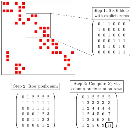
We provide an example of the prefix sum routine in a sparse matrix in Figure 3.1 and show how to use subtractions to count the number of nonzero entries in Figure 3.2.
To reflect the fact thatAmay be stored in an arbitrary sparse format, we abstract the process
of finding the indices of nonzeros within a certain range into an algorithm called
NonzerosIn-Range. NonzerosInRange(A,j,j0) returns a list of alli∈j→j0 such that A[i]6= 0. Efficient
implementations of NonzerosInRange will be discussed for various sparse formats in Section
3.2.1
We can now stateComputeX.
Algorithm 3.3. Given a sparse tensor A ∈ FI1×I2×...×IN, i, and B, compute xb(A,i) for all
N-dimensional grids b≤ B. Note that A may be stored in a sparse format, whereas all other
tensors are stored in a dense format. Require: A[i]6= 0 B ≥1 1: functionComputeX(A,i, B) 2: Z0∈Ni−B→i+B−1 3: Z0←0 4: for j∈NonzerosInRange(A,i−B,i+B−1)do 5: Z0[j]←1 6: forn∈1→N do
7: forj∈in−B+ 1→in+B−1do .Perform prefix sum
8: Z0[:| {z }, ...,:, j n ,:, ...,:]← Z0[:| {z }, ...,:, j n ,:, ...,:] +Z0[:|, ...,{z:j−1} n ,:, ...,:] 9: forb1∈1→B do 10: Z1← Z0[tb1(i1)],:| {z }, ...,: n−1 ]− Z0[hb1(i1)−1,:| {z }, ...,: n−1 ] 11: forb2∈1→B do 12: Z2← Z1[tb2(i2),:| {z }, ...,: n−2 ]− Z1[hb2(i2)−1,:| {z }, ...,: n−2 ] ... 13: forbN ∈1→B do 14: ZN ← ZN−1[tbN(iN)]− ZN−1[hbN(iN)−1] 15: X[b]← Z1N Ensure: X[b]←xb(A,i)
3.2 ComputeX 3 THE ALGORITHM
Step 1: 6×6 block
with explicit zeros 0 1 1 0 0 0 1 0 0 0 0 0 0 0 1 0 0 0 0 0 0 1 1 1 0 0 1 0 1 0 0 0 0 0 1 1
Step 2: Row prefix sum 0 1 2 2 2 2 1 1 1 1 1 1 0 0 1 1 1 1 0 0 0 1 2 3 0 0 1 1 2 2 0 0 0 0 1 2
Step 3: ComputeZ0via
column prefix sum on rows 0 1 2 2 2 2 1 2 3 3 3 3 1 2 4 4 4 4 1 2 4 5 6 7 1 2 5 6 8 9 1 2 5 6 9 11
Figure 3.1– A view of the prefix sum routine in a sparse matrix. The filled rectangles represent
nonzero elements. In this example, we want to compute the number of nonzero elements in the 6×6
block. To do so, we fill in a block with ones where our matrix has ones and zeros where it has zeros in the block. We then perform a prefix sum on the rows, then the columns. The highlighted element in step 3 is the number of nonzeros in the block.
11 3
5 3
Step 4: ComputeZ2 using column prefix sums
Z2= 11−5−3 + 3 = 6 0 1 2 2 2 2 1 2 3 3 3 3 1 2 4 4 4 4 1 2 4 5 6 7 1 2 5 6 8 9 1 2 5 6 9 11
Figure 3.2– An example of subtractions inComputeX on a matrix. First, we compute the prefix sums. In this example, we want to find the number of nonzeros in the shaded area. We compute the number of nonzeros in the sub-block by subtracting the prefix sum results from the complement of the requested sub-block in the overall block.
4 ANALYSIS
The time complexity of ComputeX is as follows:
Theorem 3.2. The algorithm ComputeX uses at most (N+ 1)(2B)N floating point operations
(flops) to computeX.
Proof. Each prefix sum takes at most (2B)Nadditions to compute, and we computeNprefix sums.
In the final loop, Zn is of size (2B)N−n. We must compute Zn at most Bn times. Therefore,
the block difference computation incurs at most PN
n=12
−n(2B)N subtractions. We must also do
one division for allBN block sizes. Therefore, the algorithm uses at most (N+ 1)(2B)N flops to
computeX, plus the time spent inNonzerosInRange.
3.2.1 NonzerosInRange
The implementation ofNonzerosInRangedepends on the initial format of the sparse matrixA.
We discuss two possible implementations to give the reader an idea of how one might implement this routine and to explain why this routine should not be costly in theory or practice.
If A is a matrix in CSR format (where nonzeros in each row are stored in sorted order of
their column index), then using a binary search within each row provides anO(Blog2(N) +B2)
implementation, where theB2term reflects the maximum number of indices that may need to be
returned.
If A is a tensor stored as an unsorted list of nonzero indices, we can perform the following
procedure. Before we run EstimateFill, we block the entire matrix Ainto blocks of size B×
...×B, and store the blocks in a sparse format (without explicit zeros). We store each block that
contains at least one nonzero in a hash table. Then, our implementation ofNonzerosInRange,
which is only ever called with ranges of size 2B×...×2B, needs only to look up the 3N blocks
which might contain zeros in the target range, scan through these blocks to find nonzeros which are actually in the target range, and return these nonzeros. The entire algorithm has a setup cost
ofO(k(A)) and an individual query cost ofO(3NBN).
4 Analysis
We use asampling procedure to repeatedly sample nonzero entries of the tensor and evaluatexb
on each selected entry, for all parameter settingsbsimultaneously. At the end of the algorithm,
we averages these values for each blocking scheme b, to obtain an estimate of fb(A) for all b.
Suppose that our procedures samples a total of S nonzeros ofA, which are located at positions
i1,i2, . . . ,iS. We want to select S as small as possible for efficiency while still having provable
guarantees on the concentration of our unbiased estimatorPjxb(ij)/S.
We give two concentration bounds for our estimator: one that assumes that the samplesij are
sampledwith replacement, using Hoeffding’s inequality [17], and an improved version where theij
are sampledwithout replacement, using the recent Hoeffding-Serfling inequality due to Bardenet
and Maillard [3]. Although the two concentration bounds are identical as the number of nonzeros
k(A) grows, the two bounds differ when the number of nonzeros is small.
4.1 A concentration bound when sampling with replacement
We make use of Hoeffding’s inequality, which we state here for completeness:
Theorem 4.1([17]). LetX1, X2, . . . , XM beM independent random variables bounded such that
0≤Xj≤1. Let X¯ = M1 PMj=1Xj be their mean. Then for any t≥0,
Pr[|X−E[X]| ≥t]≤2 exp(−2Mt2).
Observe that for any blocking scheme b and any tensor elementi, the value xb(i) is a
4.2 A concentration bound when sampling without replacement 4 ANALYSIS
independently from among the nonzeros, the random variablesxb(i1), xb(i2), . . . , xb(iS) are
inde-pendent. We can therefore apply Theorem 4.1 to obtain our first concentration bound: Theorem 4.2 (Restatement of Theorem 1.2). If we sample at least S ≥ NBN
2ε2 log 2δB
samples with replacement, then
Pr max b≤B |fb−Fb| fb ≤ε ≥1−δ . Proof. By definition,Fb=b1b2S···bN PS j=1xb(ij). By Theorem 1.1,E[Fb] =fb. xb(i1), xb(i2), . . . , xb(iS)
are independent and bounded between 0 and 1. By Theorem 4.1, we have
Pr[|Fb−fb| ≥εfb]≤2 exp(−2Sε2fb2)≤2 exp(−2Sε2/BN),
since Fb is b1b2· · ·bN times an average ofS values, each of which is at least 1/BN, since each
block has at least one nonzero entry and is of size at mostBN. By the union bound over theBN
possible blocking schemesb,
Pr max b≤B |fb−Fb| fb ≥ε ≤2BNexp(−2Sε2/BN). Therefore, ifS ≥NBN 2ε2 log 2δB , Pr max b≤B |fb−Fb| fb ≥ε ≤δ .
Note that this bound is not directly dependent onk(A). Clearly, obtaining a high probability
bound with δ ≤ 1/k(A)w for some w would indeed require dependence on k(A), albeit only
logarithmically. However, in practice a small constantδ such as 0.01 likely suffices. This bound
is quite reasonable when S k(A), the number of nonzero entries in the tensor. Because it is
constant with respect to the number of nonzeros, the bound on S could (and does, for realistic
settings of ε and δ) exceed the number of nonzeros. This is fundamental to bounds based on
Hoeffding’s inequality, and methods based on sampling-with-replacement in general. In the next section, we obtain a bound on the number of samples needed that scales “smoothly” with the number of nonzeros, and critically never exceeds it.
4.2 A concentration bound when sampling without replacement
Recall that our algorithm can be viewed as sampling a set of random locations in the tensor, and
then evaluating thedeterministic functionxb for various blocking schemesbat that location. In
the previous section, we imagined sampling the locations with replacement, so that the selected nonzeros are independent. By a stochastic domination argument, we could easily extend this bound to the case where the locations are sampled without replacement, but the bound remains
weak in the regime where the minimalS andk(A) are similar in size. Here, we use the following
recent concentration bounds for samplingwithout replacement due to Bardenet and Maillard [3]:
Theorem 4.3 (Hoeffding-Serfling inequality). Let χ={x1, x2, . . . xM} be a finite population of
M >1real points witha= minjxj andb= maxjxj. Let(X1, X2, . . . Xm)be a list of sizem < M
sampled without replacement fromχ. Then for allε >0, we have Pr 1 m m X j=1 Xj−M1 M X j=1 xj ≥ε ≤exp− 2mε2 (1−m/M)(1 + 1/m)(b−a)2 .
Here, our finite populations areχb, the images of the nonzeros under the functionsxb. Observe
that our algorithm as stated in Section 3 samples points independently, but without replacement, and so we can readily apply Theorem 4.3.
5 RESULTS
Theorem 4.4 (Restatement of Theorem 1.3). Let T =NBN
2ε2 log 2δB . If S≥S0= T−T/k(A) + p (T −T/k(A))2+ 4T(1 +T/k(A)) 2 + 2T/k(A) , then Pr max b≤B |fb−Fb| fb ≥ε ≤δ.
Proof. By Theorem 1.1,E[Fb] =fb, and so by Theorem 4.3,
Pr[Fb∈/ (1±ε)fb]≤2 exp
−(1−S/k(2ASε))(1 + 12 /S)
.
Taking the union bound over the BN such parameters, we obtain that the probability that we
have more thanεrelative error forany blocking scheme is
Pr max b≤B |fb−Fb| fb ≥ε ≤2BNexp− 2Sε2 (1−S/k(A))(1 + 1/S) ≤2BNexp− 2S0ε2 (1−S0/k(A))(1 + 1/S0) .
Substituting our expression forS0 and rearranging, we obtain that
Pr max b≤B |fb−Fb| fb ≥ε ≤δ.
5 Results
We implemented3our algorithm, which we will refer to asASX, for sparse matrices in CSR format
in C.
We chose C to provide a fair comparison to the competing algorithm described in [2], which
we will refer to asOSKI. To remove differences in speed from using different library functions, we
modifiedOSKIto use the default GNU Scientific Library (GSL) random number generator, which
is an implementation of themt19937Mersenne twister, a pseudorandom number generator which
is considered suitable for use in Monte Carlo simulations [18, 19]. To avoid differences in speed
due to different integer types, we modified bothASXandOSKIto store sparse matrix indices using
the unsigned typesize t, a macro which expands to a 64-bit unsigned quantity on our system.
We also chose C because C can efficiently execute the dense integer and floating point operations in Algorithm 3.3. An important factor in the design of this algorithm was that most of the computational work is a good target for instruction-level parallelism and cache optimizations. We have not yet fully optimized the inner kernel, but we leave this remark here to hint at future work.
5.1 Test Cases
We run our code on 5 matrices, 3 of which are matrices taken from the SuiteSparse Collection and
used by Vuduc et al. [2] to measureOSKI, and 2 of which are pathological cases we invented to
trip up bothOSKIandASXrespectively.
The three matrices taken from SuiteSparse attempt to show the performance of the fill algo-rithm over a variety of fill patterns which appear in practice.
3dtube is a matrix arising from the application of finite element analysis to a computational
fluid dynamics problem. This matrix consists mostly of 3×3 dense blocks (96% of nonzeros reside
in these blocks).
5.2 Performance Results 5 RESULTS ct20stifarises from the application of finite element analysis to a different problem, that of
structural mechanics. This matrix consists of a mix of different block sizes, mostly 3×3 and 6×6.
gupta1 is the matrix representation of a linear programming problem, and has no obvious block structure.
pathological ASX is a matrix designed to bring out the worst in ourASXalgorithm. Because the indices of nonzeros are sampled with equal probability, blocks with many nonzeros become much more likely to be sampled than blocks without nonzeros. We maximize the probability of sampling full blocks by filling them completely. We minimize the probability of sampling sparser
blocks by leaving only one nonzero in each one. We create a 1000×1000 matrix with 500 full
12×12 blocks and 500 sparse 12×12 blocks. This is a matrix which ASXshould perform poorly
on.
pathological OSKIis a matrix designed to bring out the worst in theOSKIalgorithm. Because
OSKIsamples rows with equal probability, hiding many blocks which look different from the rest of
the matrix in a single row should causeOSKIto perform poorly. This matrix is of size 10000×10000,
and the first 6 rows are dense, while all other rows have only a 1 in the first column.
5.2 Performance Results
Vuduc et al. describe how the fill heuristic is multiplied by a performance constant to create a performance heuristic. After computing the approximate fill for each blocking, the blocking with the maximum such heuristic value is chosen [2]. We can guarantee that the relative error between the estimated best performance heuristic value and the true best performance heuristic value is at most the maximum relative error in all of the estimates:
max b≤B
|fb−Fb|
fb .
Therefore, we measure the mean over several trials of the maximum relative error over all estimates. Keep in mind that if the mean maximum relative error is greater than 1, this represents a complete loss of accuracy, as a bogus algorithm which returns 0 for all estimates would achieve a better mean maximum relative error.
Each data point on the following plots represents the mean (for both maximum relative error and time) of 100 runs. All trials were performed on a Mid 2015 15-inch Retina MacBook Pro
boasting an Intel®Core™i7-4770HQ CPU @ 2.20GHz Processor with 32KB of L1 cache, 26KB of
L2 cache, 6.3MB of L3 cache, and 64B cache lines.
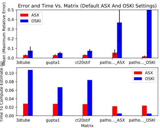
In practice, we found that the runtime and accuracy of theOSKI implementation varied
sub-stantially across matrices, even for the same recommended parameter setting ofσ= 0.02. Ideally,
sampling algorithms should be able to provide users with a consistent level of accuracy so that they can use the estimates provided with some confidence. Figure 5.1 shows the runtime and
accuracy of ASX and OSKI on all of the above matrices using default settings. We see that on
practical test cases,ASXprovides results which are twice as accurate asOSKIin half the time. We
also see that ASX performs about as well on pathological matrices as it does on practical ones,
5.2 Performance Results 5 RESULTS
3dtube
gupta1
ct20stif
patho..._ASX patho..._OSKI
0.0
0.1
0.2
0.3
0.4
0.5
Mean (Maximum Relative Error)
Error and Time Vs. Matrix (Default ASX And OSKI Settings)
ASX
OSKI
3dtube
gupta1
ct20stif
patho..._ASX patho..._OSKI
Matrix
0.00
0.02
0.04
0.06
0.08
0.10
Time To Compute Estimate (s)
ASX
OSKI
Figure 5.1– Accuracy and Time for bothASXandOSKIon several matrices (average of 100 trials,
error bars reflect one standard deviation above and below the mean). ASX parameters areε = 0.5
andδ = 0.01. OSKI parameters areσ= 0.02. In all cases, the average error due toOSKI is greater than that of ASX. ASXis faster on real-world matrices and slower on pathological cases, but unlike
OSKI,ASXprovides useful results for the pathological cases.
The variance in OSKI’s runtime made it difficult to create useful plots. Despite this difficulty,
almost all sampling algorithms, includingOSKI, provide some tradeoff between accuracy and
run-time. Even though the relationship between OSKI’s parameters and its runtime and accuracy is
unpredictable, the relationship betweenOSKI’s runtime and its accuracy is familiar. Therefore,
we show, for bothASX andOSKI, the error in the estimated fill after running these methods for
5.2 Performance Results 5 RESULTS
0.00 0.02 0.04 0.06 0.08 0.10 0.12 0.14 Time To Compute Estimate (s) 0.0 0.1 0.2 0.3 0.4 0.5
Mean (Maximum Relative Error Over Block Sizes)
Mean Maximum Relative Error Vs. Time To Compute (3dtube) ASX OSKI
0.00 0.02 0.04 0.06 0.08 0.10 0.12 0.14 0.16 Time To Compute Estimate (s)
0.0 0.1 0.2 0.3 0.4 0.5
Mean (Maximum Relative Error Over Block Sizes)
Mean Maximum Relative Error Vs. Time To Compute (gupta1) ASX OSKI
0.00
0.02
0.04
0.06
0.08
0.10
0.12
0.14
Time To Compute Estimate (s)
0.0
0.1
0.2
0.3
0.4
0.5
Mean (Maximum Relative Error Over Block Sizes)
Mean Maximum Relative Error Vs. Time To Compute (ct20stif)
ASX
OSKI
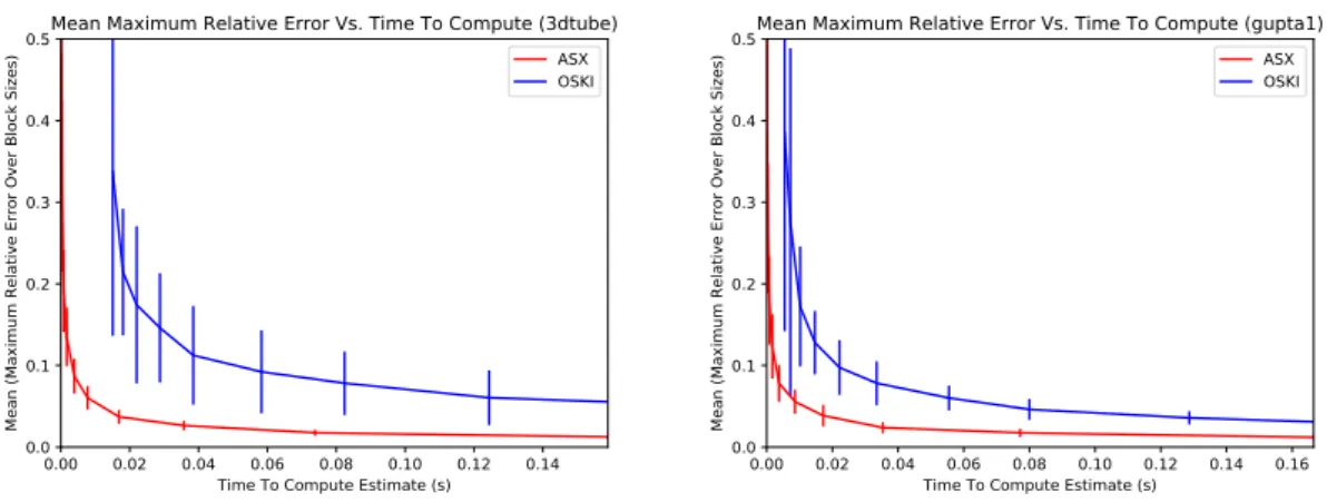
Figure 5.2– Accuracy vs. Time Tradeoffs for matrices which arise in practice (average of 100 trials,
error bars reflect one standard deviation above and below the mean). Given the same runtime,ASX
estimates the fill more accurately thanOSKIdoes in all cases.
Figure 5.2 shows the performance of the two algorithms on the matrices which arise in practice.
6 CONCLUSION
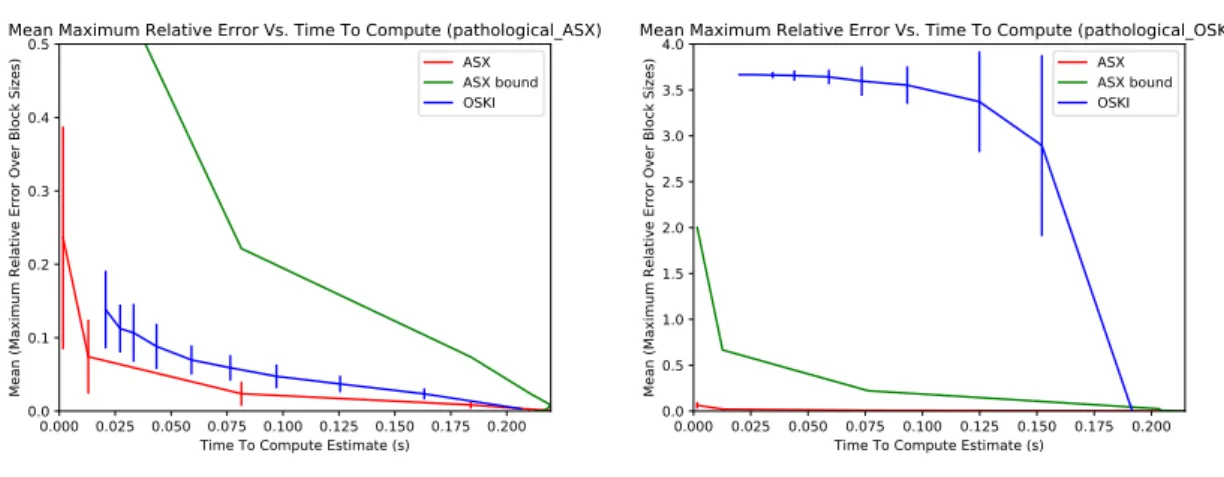
0.000 0.025 0.050 0.075 0.100 0.125 0.150 0.175 0.200 Time To Compute Estimate (s)
0.0 0.1 0.2 0.3 0.4 0.5
Mean (Maximum Relative Error Over Block Sizes)
Mean Maximum Relative Error Vs. Time To Compute (pathological_ASX) ASX
ASX bound OSKI
0.000 0.025 0.050 0.075 0.100 0.125 0.150 0.175 0.200 Time To Compute Estimate (s)
0.0 0.5 1.0 1.5 2.0 2.5 3.0 3.5 4.0
Mean (Maximum Relative Error Over Block Sizes)
Mean Maximum Relative Error Vs. Time To Compute (pathological_OSKI) ASX
ASX bound OSKI
Figure 5.3– Accuracy Vs. Time Tradeoffs for pathological cases (average of 100 trials, error bars reflect one standard deviation above and below the mean). Here we show the theoretical boundεfor
ASXcorresponding to a setting ofδ= 0.01.
Figure 5.3 shows the performance of the two algorithms on pathological cases. We ran both
ASX and OSKI to completion, meaning that both algorithms were run until they computed an
exact estimate. In both thepathological ASX andpathological OSKI cases, we find thatASX
estimates the fill more accurately in less time thanOSKI. In the pathological ASXcase, we see
thatASXperforms better thanOSKI, but the difference is smaller than in the practical cases.
For thepathological OSKIcase, we see thatOSKI fails to estimate the fill in any reasonable
runtime. The theoretical error bound ofASXapproaches zero faster thanOSKI’s empirical estimates
in thepathological OSKI case. Furthermore, in both pathological cases, the empirical error of
ASXis lower than the theoretical bound and is significantly lower than the empirical error rate of
OSKIin thepathological OSKI case.
6 Conclusion
We have shown our algorithm to be more predictable and accurate than existing approaches. Our algorithm can efficiently compute an approximation of the fill in a wide variety of circumstances.
Specifically, ASX computes the fill more accurately and faster than existing approaches on
real-world inputs and provides useful estimates of the fill in pathological test cases.
Sampling techniques are useful in autotuning since we can often sacrifice some accuracy in the heuristics for a faster autotuner runtime. As libraries for numerical computation evolve and autotuning moves from compile-time implementations to run-time implementations, developers will need heuristics whose execution time is small in comparison to that of the routine which is being tuned [20].
We have shown an example of how sampling can be applied to autotuning to efficiently produce good approximations with provable guarantees and hope that this work shows the broader potential for sampling techniques when designing autotuned numerical software. The creation of faster sampling algorithms with provable guarantees will allow library developers to write software that can more accurately specialize to user data and provide the best possible performance for their application and hardware.
6.1 Future Work
The main motivation behind the design of our algorithm was to express the problem as a dense set of operations that can be computed efficiently. We have shown that our approach is faster than existing approaches in all test cases. Future work includes a parallel implementation of both
REFERENCES REFERENCES
ASXandOSKI. Although both algorithms easily parallelize to a multicore setting, we hope to gain
even more performance through instruction level parallelism in dense operations such as the prefix sum and the differences operation.
Recall that a blocking scheme b is defined by the dimensions of each block (b1, b2, . . . , bN).
Another variant on the fill estimation problem introducesoffsets. An offset is defined by a vector
o= (o1, o2, . . . oN) such that the block indices of a nonzero elementiare defined as follows:
i1+o1 b1 , i2+o2 b2 , ..., iN +oN bN .
Both the ASXandOSKI algorithm currently estimate the fill using only block sizes, but some
matrices may have smaller fills in an offset blocked sparse matrix. Because most of the information
needed to compute xb,o is already computed when we computexb, we can compute the fill over
all possible combinations of block sizes and offsets by modifying only the differences operation.
Another extension to the problem is to limit the volume of the blocking scheme. That is, for
any blocking scheme b, we require b1×b2×. . .×bN ≤ V for some maximum volume V. For
volume to be a nontrivial quantity, we would set it to less thanBN whereB is the maximum size
of a block dimension. If the blocks are too large, the performance of tensor operations declines as we are required to fill in more explicit zeros. Thus, we are unlikely to choose these block sizes
after calculating the fill. If the volume is limited to V, then the expected value of xb(A,i) on a
randomly choseni is at least 1/V. Thus, limiting the volume increases the lower bound on the
expected value of the fill, meaning that the theoretical accuracy guarantee will get closer to the empirically measured accuracy.
References
[1] Rich Vuduc, James W Demmel, Katherine A Yelick, Shoaib Kamil, Rajesh Nishtala, and Benjamin Lee. Performance optimizations and bounds for sparse matrix-vector multiply. In Supercomputing, ACM/IEEE 2002 Conference, pages 26–26. IEEE, 2002.
[2] Richard Vuduc, James W. Demmel, and Katherine A. Yelick. OSKI: A library of automatically
tuned sparse matrix kernels. InProc. SciDAC, J. Physics: Conf. Ser., volume 16, pages 521–
530, 2005.
[3] R´emi Bardenet, Odalric-Ambrym Maillard, et al. Concentration inequalities for sampling
without replacement. Bernoulli, 21(3):1361–1385, 2015.
[4] Yousef Saad. Iterative methods for sparse linear systems. SIAM, 2003.
[5] Aydin Bulu¸c, Jeremy T Fineman, Matteo Frigo, John R Gilbert, and Charles E Leiserson. Parallel sparse matrix-vector and matrix-transpose-vector multiplication using compressed
sparse blocks. InProceedings of the twenty-first annual symposium on Parallelism in
algo-rithms and architectures, pages 233–244. ACM, 2009.
[6] Shaden Smith and George Karypis. Tensor-matrix products with a compressed sparse tensor. InProceedings of the 5th Workshop on Irregular Applications: Architectures and Algorithms, page 5. ACM, 2015.
[7] Brett W Bader and Tamara G Kolda. Efficient matlab computations with sparse and factored
tensors. SIAM Journal on Scientific Computing, 30(1):205–231, 2007.
[8] Fredrik Kjolstad, Shoaib Kamil, Stephen Chou, David Lugato, and Saman Amarasinghe. The
tensor algebra compiler. 2017. MIT-CSAIL-TR-2017-003http://hdl.handle.net/1721.1/
107013.
[9] Richard W. Vuduc. Automatic performance tuning of sparse matrix kernels. PhD thesis,
REFERENCES REFERENCES
[10] Samuel Williams, Leonid Oliker, Richard Vuduc, John Shalf, Katherine Yelick, and James Demmel. Optimization of sparse matrix–vector multiplication on emerging multicore
plat-forms. Parallel Computing, 35(3):178–194, 2009.
[11] Buse Yilmaz, Bari¸s Aktemur, Mar´ıA J. Garzar´an, Sam Kamin, and Furkan Kira¸c. Autotuning
runtime specialization for sparse matrix-vector multiplication. ACM Trans. Archit. Code
Optim., 13(1):5:1–5:26, March 2016.
[12] Richard Vuduc and Hyun-Jin Moon. Fast sparse matrix-vector multiplication by exploiting
variable block structure.High Performance Computing and Communications, pages 807–816,
2005.
[13] Alfredo Buttari, Victor Eijkhout, Julien Langou, and Salvatore Filippone. Performance
opti-mization and modeling of blocked sparse kernels. The International Journal of High
Perfor-mance Computing Applications, 21(4):467–484, 2007.
[14] Jee W Choi, Amik Singh, and Richard W Vuduc. Model-driven autotuning of sparse
matrix-vector multiply on gpus. InACM sigplan notices, volume 45, pages 115–126. ACM, 2010.
[15] Eun-Jin Im, Katherine Yelick, and Richard Vuduc. extscSparsity: Optimization framework
for sparse matrix kernels. Int’l. J. High Performance Computing Applications (IJHPCA),
18(1):135–158, February 2004.
[16] Eun-Jin Im and Katherine Yelick. Optimizing sparse matrix computations for register reuse
in sparsity. Computational Science?ICCS 2001, pages 127–136, 2001.
[17] Wassily Hoeffding. Probability inequalities for sums of bounded random variables. Journal
of the American statistical association, 58(301):13–30, 1963.
[18] Makoto Matsumoto and Takuji Nishimura. Mersenne twister: a 623-dimensionally
equidis-tributed uniform pseudo-random number generator. ACM Transactions on Modeling and
Computer Simulation (TOMACS), 8(1):3–30, 1998.
[19] Makoto Matsumoto. Mersenne Twister with improved initialization.http://www.math.sci.
hiroshima-u.ac.jp/~m-mat/MT/MT2002/emt19937ar.html, 2002. Online; accessed 14 May 2017.
[20] Jack Dongarra and Victor Eijkhout. Self-adapting numerical software for next generation
applications.International Journal of High Performance Computing Applications, 17(2):125–