THESIS FOR THE DEGREE OF DOCTOR OF PHILOSOPHY
Modelling and Inference for
Spatio-Temporal Marked Point
Processes
Ottmar Cronie
Department of Mathematical Sciences
Chalmers University of Technology and University of Gothenburg Göteborg, Sweden 2011
ISBN 978-91-7385-586-0 c
Ottmar Cronie, 2011
Doktorsavhandlingar vid Chalmers Tekniska Högskola ISSN 0346-718X
Ny serie nr 3267
Department of Mathematical Sciences
Chalmers University of Technology and University of Gothenburg SE-412 96 Göteborg
Sweden
Telephone +46 (0)31-772 1000
Modelling and Inference for Spatio-Temporal Marked
Point Processes
Ottmar Cronie
Department of Mathematical Sciences
Chalmers University of Technology and University of Gothenburg
Abstract
This thesis deals with inference problems related to the growth-interaction process (GI-process). The GI-process is a continuous time spatio-temporal point process with dynamic interacting marks (closed disks), in which theimmigration-death process(ID-process) controls the arrivals of new marked points as well as their potential life-times. The data considered are marked point patterns sampled at fixed time points and the main area of application of the GI-process is the dynamical modelling of the trees in a forest stands.
The parameters related to the development of the marks are estimated using the least-squares (LS) approach. The death rate, which is assumed to be a function of the mark sizes, and the arrival intensity and are estimated by (approximate) maximum likelihood (ML) methods. We also propose three edge correction methods for discretely sampled (marked) spatio-temporal point processes. The edge correction methods together with the LS approach are applied to fit the GI-process to a forest stand of Scots pines.
We derive the transition probabilities of the (Markovian) ID-process, which form the likeli-hood function of its two parameters. We further reduce the ML-problem from two dimensions to one dimension. Given an equidistant sampling scheme and some conditions for the pa-rameter space, we manage to prove the consistency and the asymptotic normality of the ML-estimators. The results are also evaluated numerically.
Measurements of locations and radii at breast height (rbh) made at 3 different time points of the individual trees in 10 Swedish Scots pine stands, are modelled spatio-temporally by the GI-process. A new location assignment strategy and a more flexible function for the open-growth (growth in absence of competition) are suggested in order to improve the fit. A linear relationship is found between the site productivity index (fertility) and the sizes of the trees. This relationship is exploited in the estimation of the carrying capacity parameter (theoretical upper bound for the radii). We also test the goodness-of-fit of the fitted model in terms of prediction.
By adding scaled continuous white noise to the mark growth equations, we obtain a system of stochastic differential equation (SDEs) for the mark growth. We consider the case where there is no interaction present and the mark SDEs are independent Cox-Ingersoll-Ross SDEs. Closed form expressions are available both for the transition densities and the stationary distributions. Under the assumption that the mark processes are stationary, consistency and asymptotic normality of the ML-estimators of the parameters are proved.
Keywords: Asymptotic normality, Consistency, Cox-Ingersoll-Ross process, Diffusion pro-cess, Edge correction, Goodness-of-fit, Richards growth function, Growth-interaction propro-cess, Immigration-death process, Least squares estimation, Markov process, Maximum likelihood estimation, Open-growth, Spatio-temporal marked point process, Stationarity, Stochastic differential equation, Transition density.
These last five years have been the most happy, interesting, challenging and rewarding years of my life! When entering the process of writing a PhD thesis, it is impossible to imagine what one will go through on such a journey. I must admit that, at times, I have also felt quite alone in the process, thinking that no one could relate to what I was going through emotionally. However, I now realize that I was very wrong in that respect. All the people who, in one way or another, have been a part of my life throughout this process have not only understood me, but they have supported me and cared about me (probably more than I deserved). This is my opportunity to pay my respect to all of you and thank you, from the bottom of my heart :)
To start with I would like to thank my advisor Aila Särkkä. Words truly are insuf-ficient for express the gratitude that I feel. I would truly like to thank you for the constant support, encouragement and inspiration given to me during these past years! What probably makes me the happiest, however, is the true friendship that we have developed!
I would further like to thank my co-advisors Jun Yu and Anastassia Baxevani. Thank you for being good mentors and colleagues, but most importantly, thank you for being good friends! I have truly learnt a great deal from you!
To one of my co-authors and colleagues, Kenneth Nyström, thank you for these last couple of years. It has been nice working with you and learning from you.
Other people who I would like to thank and show gratitude for ideas and inspiration related to the writing of this thesis include: Claudia Redenbach, Eric Renshaw, Gerald van den Boogaart, Patrik Albin, Peter Guttorp and Serik Sagitov.
Also, a general thank you goes out to all the people at the department of Mathematical Sciences in Gothenburg and a few of you deserve special attention: Daniel, Dmitrii, Frank and Sofia, thank you for these years of happiness and friendship ;) Related to my work (socially or workwise), other people I would like to thank on a personal level include Alexandra, Anders, Carl, Elisabeth, Emilio, Erik, Erik, Fredrik, Hans, Hermann, Hossein, Igor, Jacques, Johan, José, Jovan, Kerstin, Lotta, Magnus, Malin, Martin, Marianne, Marie, Mattias, Michael, Tommy and Torbjörn.
To all my friends outside the department. Thank you for your love, friendship and support! Some of you deserve special attention: Adam, Alain, Alma, Anders, An-dreas, Bryan, Daina, Daniel (all of you), Farhad, Felicia, Felipe, Henrik, Hilma, Joel, Jonathan, Kajsa, Laszlo, Marcel, Maria, Mauri, Mattias, Niklas, Raphael, Rikard, Sandra, Sara, Serkan and Simon.
Finally, to the people who mean the most to me. My family. I love you. Thank you for your eternal love and support! You have been with me all the way and I cannot thank you enough for everything. Bobo, thank you for your support and love! Greetings from Dr Cronie (to be)...
List of Papers
This thesis includes the following papers. Paper I. Cronie, O., Särkkä, A. (2011).
Some edge correction methods for marked spatio-temporal point process models. Computational Statistics & Data Analysis 55, 2209-2220. Paper II. Cronie, O., Yu, J. (2010).
The Discretely Observed Immigration-Death Process and its Maximum Likelihood Estimation. Preprint.
Paper III. Cronie, O., Nyström, K., Yu, J. (2011).
Spatio-Temporal Modelling of Swedish Scots Pine Stands. Preprint. Paper IV. Cronie, O. (2011).
Likelihood Inference for a Stochastic Version of the Spatio-Temporal Growth-Interaction Process. Preprint.
Contents
1 Introduction 1
2 The process 5
2.1 The immigration-death process . . . 5
2.2 The GI-process . . . 7
2.2.1 The natural death rate . . . 9
2.2.2 Remarks about the competitive death . . . 10
2.3 The stochastic GI-process . . . 10
2.3.1 Distributional properties of the SG-process . . . 13
3 Parameter estimation 17 3.1 Estimation of the GI-process parameters . . . 17
3.1.1 Estimation of the growth and interaction parameters . . 17
3.1.2 Estimation of the death and arrival rates . . . 20
3.2 Estimation in the ID-process . . . 21
3.2.1 The ML-estimators . . . 22
3.2.2 Asymptotic properties of the ML-estimators . . . 23
3.3 Maximum likelihood inference in the SG-process . . . 23 vii
3.3.1 ML-estimation: M0
i =M0∈R+ . . . 24 3.3.2 ML-estimation: M0
i ∼π . . . 25
3.3.3 Asymptotic inference under stationarity . . . 25 3.4 Spatio-temporal edge correction . . . 27
4 Future work and extensions 29
5 Summary of Papers 33
Paper I: Some edge correction methods for marked spatio-temporal point process models . . . 33 Paper II: The Discretely Observed Immigration-Death Process and
its Maximum Likelihood Estimation . . . 34 Paper III: Spatio-Temporal Modelling of Swedish Scots Pine Stands 34 Paper II: Likelihood Inference for a Stochastic Version of the
Spatio-Temporal Growth-Interaction Process . . . 35
A Appendix 37
Chapter 1
Introduction
In many different instances in our surrounding world we find point patterns of different kinds. Such patterns include galaxy locations, locations of earthquake epicentres, locations of cell centres and locations of trees in a forest stand. In order to help analysing point patterns the field of spatial statistics has lent a helping hand and has simultaneously also been developing through it. The field of spatial statistics incorporates a few different disciplines within the field of stochastic mathematics and in this thesis we will focus on the parts played by
stochastic geometry(the study of random geometrical objects) andspatial point processes (the study of random point structures) (see e.g. [7, 10, 20, 21, 33]). Sometimes one does not solely record the locations of the points in a point pattern but also some additional features connected to each point, such as the radii of the trees in a forest stand or the amount of seismic energy in earthquakes. This additional variable, called amark, can often be quite helpful in explaining the behaviour of the point pattern in question. When focusing on the statistical analysis of these point patterns or marked point patterns, we employ spatial point processes or marked spatial point processes, respectively (see e.g. [7, 12, 20, 33, 34]). However, to a large extent, the field of spatial (marked) point processes has mainly concentrated on treating marked point patterns within a purely spatial framework. In such a setting one fully ignores that the patterns studied, in fact, almost always are results of evolutionary processes in which the changes occurring among the marks are time dependent. Such situations motivate a change of regime to an approach where one instead considersspatio-temporal marked point processes (see e.g. [14, 24, 36]). To fully take the evolution of these marked patterns into consideration it is reasonable to demand that the models describing them should incorporate interaction
between marks during the development phases.
The application motivating the work presented in this thesis is found in forestry. Treating a forest stand which is recorded at a specific time point as a static entity, thus ignoring the temporal aspects, the literature offers a wide range of statistical tools for analysing and drawing conclusions about its inherent features, whether one includes marks or not (see e.g. [12, 20, 16, 34] to mention a few). However, here we are interested in modelling the development of a forest stand in both space and time. Figure 1.1 illustrates the type of recorded time series of marked point patterns we refer to – a data set of Swedish Scots pines recorded in 1985, 1990 and 1996 where we have scaled the radii (our marks) for more clear visualisation.
−10 −5 0 5 10 −10 −5 0 5 10 Pines 1985 −10 −5 0 5 10 −10 −5 0 5 10 Pines 1990 −10 −5 0 5 10 −10 −5 0 5 10 Pines 1996
Figure 1.1: Locations and sizes (measured in metres) of Swedish Scots pines recorded in 1985(left),1990(middle) and1996(right). The radii of the trees (marks) are scaled by a factor of 10.
A clear risk when formulating the type of spatio-temporal models we are inter-ested in is that the models easily become too involved and we loose both trans-parency, interpretability and tractability (see e.g. [15]). A spatio-temporal marked point process which manages well to describe this type of spatio-temporal behaviour of a marked population is the so calledGrowth-Interaction process (GI-process) (see [28, 29, 32] or Papers I and III), which is a combi-nation of stochastic and deterministic components (note that it has also been referred to as theRenshaw-Särkkä growth-interaction model). It has been used to study, among other things, the development of forest stands [32]. Since this model, in spite of being very flexible, is both tractable and easily interpreted it is quite natural to further assess its potential. In the coming chapters we will present and discuss the GI-process together with different statistical tools developed for it (and other models of this type) and further developments of it.
3 only, the stochastic process controlling the arrivals and deaths of new marked points in time, but also the mechanism controlling the growth of and interaction between the marks. In the GI-process the arrivals and deaths are controlled by a so-calledimmigration-death process (ID-process) – a continuous time Markov chain.
In both Paper I and Paper II estimators for the two parameters of the ID-process are given and in Paper I we also recall how the growth and interaction parameters of the GI-process are estimated. Additionally in Paper I, for the Scots pine data in Figure 1.1, we evaluate some of the estimators of the GI-process in the context of the edge correction methods developed in Paper I. In Paper II, where the likelihood estimation of the discretely sampled ID-process is tackled, we prove that the obtained likelihood estimators are both consistent and asymptotically normally distributed. Having obtained ideas in Paper I about how to improve the fit of the GI-process, in Paper III the model is altered in the way individuals (trees) are assigned locations in the study region and in the way they grow in absence of competition (open-growth). As the main objective of Paper III is to evaluate further how the GI-process fits Scots pine data, we fit the model to a series of pine data sets of the type presented in Figure 1.1 and finally exploit a set of goodness-of-fit procedures (spatial and forestry related) to assess the fit of the predicted model. In Paper IV we modify the model by adding scaled white noise to the equations which govern the growth of the marks, and hereby the mark growth will be driven instead by a system of stochastic differential equations (SDEs). By utilizing the findings in Paper II and properties of the mark SDEs, under the restriction that there is no interaction present among the individuals, a full likelihood estimation procedure is developed in Paper IV. By putting some additional restrictions on the SDEs, consistency and asymptotic normality are proved.
Chapter 2
The process
We will here define the spatio-temporal marked point process ΦM(t) =
{[Xi, Mi(t)] : i ∈ Ωt}, which we refer to as the Growth-Interaction process
(GI-process) (see e.g. [32], Paper I and Paper IV). Consider a spatial study region W, which either is given by a subset of the Euclidean space R2 (or
possiblyR3) or by a torus (see e.g. [12]). As timet ∈[0, T)⊆[0,∞)passes,
individuals (marked points) arrive to W at random times and receive loca-tions Xi ∈ W. Additionally, as time passes, the dynamical and interacting
marks Mi(t) change size until they die and leave W. In order to keep track
of which individuals are alive at a given time, we define the index process
Ωt={indices of individuals alive at timet}. Before giving a detailed
descrip-tion of the GI-process, however, we first describe the immigradescrip-tion-death pro-cess, {N(t)}t≥0, which controls the arrivals and deaths.
2.1
The immigration-death process
The immigration-death (ID) process, {N(t)}t≥0, is a time-homogeneous ir-reducible continuous-time Markov chain (see e.g. [23]) where the possible states for which transitions i→j are possible are supplied by the state space
E =N={0,1, . . .}. It is governed by the parameter pairγ= (α, µ)which we
here assume to take values in some compact parameter space Γ⊆R2+.
One way of viewing{N(t)}t≥0 is to treat it as a special case of a birth-death 5
process, for which the infinitesimal transition probabilities are given by pij(t;γ) :=P(N(h+t) =j|N(h) =i) = λit+o(t) ifj=i+ 1 1−(λi+µi)t+o(t) ifj=i µit+o(t) ifj=i−1 o(t) if|j−i|>1,
where the birth rates are given byλi=α,i= 0,1, . . ., and the death rates are
given byµi =iµ, i = 0,1, . . ., (see [17], p. 268-270). Within this framework
the interpretation of{N(t)}t≥0 is the following. By letting the arrivals of new individuals to a population occur according to a Poisson process with intensity
αand upon arrival assigning to all individuals independent and exponentially distributed lifetimes with mean1/µ, N(t) gives us the number of individuals alive at timet. Another possibility is to view it as anM/M/∞queuing system; each customer (arriving according to a Poisson process with intensityα) is being handled by its own server so that its sojourn time in the system is exponential with intensityµand independent of all other customers.
Being a Markov process, the finite dimensional distributions of{N(t)}t≥0 are controlled by its transition probabilities,pij(t;γ)which are given in Paper II.
Proposition 2.1.1 (Paper II). The transition probabilities of the ID-process are given by convolutions of Poisson densities and Binomial densities, i.e.
pij(t;γ) = fP oi(ρ)∗fBin(i,e−µt) j = j X k=0 fP oi(ρ)(k)fBin(i,e−µt)(j−k) = i∧j X k=0 fP oi(ρ)(j−k)fBin(i,e−µt)(k) = e −α µ(1−e −µt) j! j X k=0 α µ k j k e−(j−k)µt (1−e−µt)j−2k−i i! (i−(j−k))! where i, j ∈ E = N, γ = (α, µ) ∈ Γ ⊆ R2+, f
P oi(ρ)(·) is the Poisson density
with parameter ρ = αµ(1−e−µt), and f
Bin(i,e−µt)(·) is the Binomial density
with parametersiand e−µt. Moreover, we have that the probability generating
function (p.g.f.) of(N(s+t)|N(s) =i)is given by
Gi(s;γ) = 1 + (s−1) e−µtieρ(s−1) (2.1)
and
E[N(s+t)|N(s) =i] = ie−µt+ρ (2.2) E[N2(s+t)|N(s) =i] = i(i−1) e−2µt+(1 + 2ρ)ie−µt+ρ2+ρ.
2.2. The GI-process 7 The interpretation ofpij(t;γ)is quite clear. Note that
fP oi(ρ)(j−k) = P(j−knew arrivals during(h, h+t))
fBin(i,e−µt)(k) = P(kof theiindividuals alive at timehsurvive(h, h+t)),
so that pij(t;γ) expresses the sum of the probabilities of all possible ways
in which we can decrease i individuals to j individuals. Furthermore, when
i≤j, we get thatpij(t;γ)simply represents the convolution of theBin(i,e−µt)
-density and the P oi(ρ)-density. One can easily show that for the marginal distributions of{N(t)}t≥0 we have thatP(N(t) =j|N(0) = 0) = e−ρρj/j!, i.e.
(N(t)|N(0) = 0)∼P oi α µ(1−e
−µt), and that (N(t)
|N(0) = 0)→d P oi(α/µ)
as t → ∞. Note that this invariant distribution is unique due to the positive recurrence, and it is also the same as its asymptotic distribution since every asymptotic distribution is an invariant distribution.
Proposition 2.1.2. The ID-process is ergodic with invariant distribution πN
given by the Poisson distribution with meanα/µ, i.e.πN(·) =P(P oi(α/µ)∈ ·).
A further characterisation of{N(t)}t≥0which sometimes is useful to exploit is to consider{N(t)}t≥0 as a Markov jump process (see Paper II).
Proposition 2.1.3 (Paper II). Let γ = (α, µ) ∈ Γ ⊆ R2+. {N(t)}
t≥0 is a
Markov jump process with state space E=N, jump intensity function
λ(γ;i) =α+µi, i∈E, and transition kernel r(γ;·) ={r(γ;i, j) :i, j∈E}, where
r(γ;i, j) = 1
α+µi(α1{j=i+ 1}+µi1{j=i−1}), i, j∈E.
2.2
The GI-process
The processΦM(t) ={[Xi, Mi(t)] :i∈Ωt}can be described as follows. As time
elapses, the arrivals in time of new individuals toW ⊆R2 and the time these
individuals live inW are governed by an ID-process,N(t), having arrival/birth rateαν(W)and death rateµ, whereν(·)denotes volume inR2. Furthermore,
for the N ∼P oi(αν(W)T) individuals who arrive during[0, T), upon arrival at times B1, . . . , BN they are assigned locationsXi ∈W (precise description
given below) and initial marks Mi(Bi) = Mi0, i = 1, . . . , N, with the latter
taken either as some fixed positive value (as will be the case here), or as a value drawn from some suitable distribution ([32] considers M0
> 0). When an individual’s (Exp(µ)-distributed) life time has expired at timeDiwe say that its has suffered a natural death and we set its size to 0.
Once individuali has arrived it starts growing deterministically according to
Mi(t) = Mi0+ Z t Bi dMi(s), Bi≤t≤Di, (2.3) where dMi(t) = f(Mi(t);θ)dt− X j∈Ωt j6=i h(Mi(t), Mj(t), Xi, Xj;θ)dt.
Here Ωt = {i∈ {1, . . . , N}:individual iis alive at timet}, θ is a
parame-ter vector, the function f(Mi(t);θ) determines the open-growth of mark i
(growth in absence of competition with other (neighbouring) individuals) and
h(Mi(t), Mj(t), Xi, Xj;θ)is a function handling the individual’s spatial
(pair-wise) interaction with other individuals. We note that as a radius/markMi(t)
changes with time, also the closed disk BXi[Mi(t)] with centreXi and radius Mi(t), which denotes the occupied space, will change in size.
In addition to the natural death, an individual can diecompetitively which we consider to happen as soon asMi(t)≤0, and the we set Mi(t) = 0 once this
happens.
In Papers I and IV we assign the locations to the individuals according to
Xi ∼U ni(W). We note that for this choice, when we ignore the competitive
deaths, at each fixed timet the locations form a spatial Poisson process with intensity αµ(1−e−µt), which is restricted to W. In Paper III, however, we letXi ∼U ni(W \Si∈Ωj∈ΩBi BXj[Mj(Bi)]), i.e. we let the location of the ith
individual be uniformly distributed on the part ofW which is not covered by other trees.
We note that in the case of no interaction, i.e. whenh(·) = 0, expression (2.3) turns intodM(t)/dt=f(M(t);θ),M(0) =M0, which hasM(t)as its solution (for simplicity we here writeM(t)forMi(t)). The literature offers a wide range
of possible choices for the growth function (see e.g. [31]), and one of the models considered in this thesis is the Richards growth function (see e.g. [28, 31]), which is given by dM(t) dt =f(M(t);θ) = λ δM(t) K M(t) δ −1 ! , M(t) = K1 +(M0/K)δ−1 e−λt1/δ,
2.2. The GI-process 9 which is a strictly increasing growth function with carrying capacity (upper bound/asymptote)K >0and growth ratesδ6= 1andλ >0. If we setδ=−1, we obtain as special case the so called logistic growth function. The logistic growth function has been considered in most of the papers which deal with the GI-process (see e.g. [32] or Paper I), and the more general Richards growth function has been employed in both [28] and in Paper III for the modelling of Scots pine stands.
Just as for the individual growth function, the possible choices of spatial inter-action functions are many (c.f. [22, 28, 32] for examples of interinter-action functions and related discussions). One example is given by (see [32])
h(Mi(t), Mj(t), Xi, Xj;θ) =c1BXi[rMi(t)]∩BXj[rMj(t)]6=∅ ,
where 1{A ∈ ·} denotes the indicator function for the set A, c ∈ R is the
force of interaction and r > 0 is the scale of interaction. Furthermore, the closed diskBXi[rMi(t)]with centreXi and radiusrmi(t)is referred to as the
’influence zone’ of individual i. Since competition for resources takes place only within influence zones ([3, 37]), individuals i and j will compete only when their influence zones intersect, i.e. whenBXi[rMi(t)]∩BXj[rMj(t)]6=∅.
This symmetric interaction function has the effect that small individuals have the same impact on large (neighbouring) individuals as the large individuals have on small individuals. Unless our forest stand consists of trees of similar size, this interaction function becomes unrealistic. In order to circumvent this problem we here consider instead the so called area interaction function, given by h(Mi(t), Mj(t), Xi, Xj;θ) =c ν BXi[rMi(t)]∩BXj[rMj(t)] ν(BXi[rMi(t)]) , (2.4)
This non-symmetric soft core interaction has the effect that large marks in-fluence small marks more than the other way around, yet allowing the small marks to play their part. This interaction model is more realistic in tree mod-elling applications than symmetric interaction models (see [28, 32]). Depending on the choice of parameters, this area interaction function has the ability to generate regular as well as aggregated point patterns (despite the possible un-derlying uniform distribution of the locations) [27]. Note that the parameterr
determines how large the range of interaction is and cmainly determines how regular the point patterns are.
2.2.1
The natural death rate
As previously mentioned the so called natural deaths are governed by the death process part of the ID-process. In situations where it seems plausible that the
natural deaths depend on an individual’s size, we may let the death rate be given by some functionµη(·),µ >0, whereη(·)is a function of the marks. This means that as time passes the Exp(µη(Mi(t)))-distributed remaining lifetime
of an individual will change with its size. An alternative way of expressing the behaviour of the death process is to say that the conditional probability that an individualidies naturally during(t, t+dt), givenMi(t), equalsµη(Mi(t))dt+
o(dt). Note that if η(·)≡1, we retrieve the ordinary ID-process. In Paper I, we choose to evaluate the GI-process under η(Mi(t)) = 1/(1 +Mi(t))which
implies that individuals become more viable as they grow; a choice motivated by our forestry applications. In Papers II and IV, as well as in [27, 28, 29, 32] the model is chosen to haveη(·)≡1.
2.2.2
Remarks about the competitive death
As previously mentioned, one of the possible death occurrences present in the GI-process is the competitive death. Consider the infinitesimal-size interval
(t, t+dt)and recall that we classify an individual as having died from compe-tition in(t, t+dt)if Mi(t)>0 and Mi(t+dt)≤0. Let us call this scenario
1. Consider now an alternative approach, which we call scenario 2, where the individual suffers a competitive death ifMi(t)>0anddMi(t)<0. Now a
rea-sonable question emerges, namely, which of the two scenarios should be used to represent competitive/interactive death for tree data. In a tree stand model one could argue that scenario 1 is a more appropriate view than scenario 2 since trees do not disappear immediately after they die. This thus indicates that they should not be removed as soon asdMi(t)<0, since dead trees occupy
the ground where they have been standing some time after their deaths. Also, to some extent, dead trees inhibit the nutrient access and light absorption of other trees close to it. Furthermore, it is not reasonable that a new tree would end up very close to the centre of a one. Although a bit artificial in its nature we thus have chosen to use of scenario 1 to represent competitive deaths, just as in [32].
2.3
The stochastic GI-process
In the case where the mark equations of expression (2.3) are instead given by stochastic differential equations (SDEs), we refer to ΦM(t) = {[Xi, Mi(t)] :
i ∈ Ωt} as the spatio-temporalstochastic growth-interaction process. In the
simplified case where there is no interaction between the individual, i.e.h(·) = 0, we will simply refer to ΦM as the spatio-temporal stochastic growth (SG)
2.3. The stochastic GI-process 11 process. Note that in this case there is no competitive death.
We buildΦM in two steps: The underlying marked point processΦ(t), governs
the locations of the individuals onW as well their arrival times and lifetimes, and the marking process, which may be regarded as an extension ofΦ, assigns the set of processes which control the growth of the marks (disks)BXi[Mi(t)].
We start by describing the underlying processΦ. Consider an ID-processN(t)
which controls the arrival times B1, . . . , BN, lifetimes L1, . . . , LN and death
timesDi= min(Bi+Li, T) = (Bi+Li)∧T of theN= Φ(T)∼P oi(αT ν(W))
individuals who arrive toW at the locationsXi∼U ni(W). The processΦ(t)is
given by the marked Poisson processB1, . . . , BN on[0, T)for which the marks
are given by the pairs (Li, Xi)(note that conditional onN,Bi ∼U ni(0, T)).
Note that hereΩt={i∈ {1, . . . , N}:t∈[Bi, Di]},Ω0=∅, andN(t) =|Ωt|.
We now turn to the second part ofΦM. Given some suitable diffusion coefficient
σ(x)and independent standard Brownian motionsWi(t),i= 1, . . . , N, we have
that, loosely speaking, the mark radii are controlled by the system of SDEs
(dM1(t), . . . , dMN(t)), where dMi(t) = f(Mi(t);θ)dt− X j∈Ωt j6=i h(Mi(t), Mj(t), Xi, Xj;θ)dt +σ(Mi(t))dWi(t), andMi(t) = 0fort /∈[Bi, Di].
In the special case of the SG-process, which is studied in Paper IV, we let
f(x) =λ(1−x/K),h(·) = 0andσ(x) =σ√x, whereby we obtain a system of independent (time-shifted) Cox-Ingersoll-Ross (CIR) processes for the growth of the marks (see e.g. [6, 13, 19]). We make this precise by letting t ∈ [0, T)
denote our global time and consider the ith CIR-process{Yi(t)}t∈[0,T) where, given Yi(0) =Mi0 and the Brownian motionWi(t), the SDE generating Yi(t)
is given by
dYi(t) = λ(1−Yi(t)/K)dt+σ p
Yi(t)dWi(t), (2.5)
so that its integral form is given by
Yi(t) = Mi0+ Z t 0 λ 1−YiK(s) ds+ Z t 0 σpYi(s)dWi(s). (2.6)
By then lettingτi(t) =t−Bi be ourithlocal time and defining
Mi(t) =
Yi(τi(t)) fort∈[Bi, Di]
we have expressedMi(t)by means of the global time scale.
The parameters(λ, K, σ)∈Θλ×ΘK×Θσ ⊆R3+ in this mean-reverting SDE control different aspects of the growth: Thediffusion coefficient σcontrols the magnitude of the random individual fluctuations of the radii. The interpreta-tion of the remaining two parameters becomes most clear by noticing thatYi(t)
is a so called mean-reverting process: AsYi(t)starts to move away from its long
term equilibrium K, the drift term starts pulling it back towardsK and the speed at which this occurs is given byλ/K. Related to this interpretation we find that if we setσ= 0in expression (2.5), we retrieve the GI-process (without interaction) and the size development of the disks will comprise the differen-tial equation dYi(t) = λ(1−Yi(t)/K)dt. This differential equation is often
referred to as the linear growth function (see e.g. [28, 32]) and in this setting the parameter λis referred to as the (individual) growth rate and recall that the upper boundKis the carrying capacity. In conclusion,ΦM is controlled by
the parameter vectorθ= (λ, K, σ, α, µ)∈Θ = Θλ×ΘK×Θσ×Θα×Θµ ⊆R5+. We note that we also may treatΦM(t)as a multivariate (N-dimensional)
dif-fusion (hence a Markov process), for which all components are independent, stopped and time-shifted CIR-processes.
Regarding the initial size Mi(Bi) = Yi(0) = Mi0, a few different options are
available. As previously mentioned, the choices M0
i ≡M0 ∈ R+ and Mi0 ∼
U ni(0, ), >0, have already been explored (see e.g. [32] and Paper I). Here, however, we also have the further option to sample each Mi(Bi) from the
stationary distribution of Yi, which turns the radius diffusion processes into
strictly stationary processes.
It is also possible to represent ΦM as a spatial entity, under the condition
thatT <∞. By restricting a homogeneous spatial Poisson process onR2with
intensityαT toW ⊆R2(see e.g. [10, 12, 30, 33]), we obtain the Poisson process
Φ0 =
{X1, . . . , XN} with intensity measureΛ(B) =αT ν(B∩W), B∈ B(R2),
whereν(·)denotes Lebesgue measure andB(R2)are the Borel sets in R2. By
now consideringΦM ={[Xi, Mi([0, T);Bi, Li)]}Ni=1, which is a marked version
ofΦ0such that theith mark is given by the random elementM
i([0, T);Bi, Li) :
X →Vi={f ∈C[0+,T): supp(f) = [Bi, Di]}, where C[0+,T)={f : [0, T)→R+:
f >0, f continuous} and supp(f) denotes the support of the function f, we have obtained a different representation of the SGI-process. Note thatΦM is a
marked spatial Poisson process for which the marks are random elements which take values in the function space {f ∈C[0+,T) : supp(f)⊆ [0, T)}, and in the case of the SGI-process these random elements are dependent.
2.3. The stochastic GI-process 13
2.3.1
Distributional properties of the SG-process
We give here some results concerning different properties of the CIR-process (they can be found in e.g. [6, 19]) and then turn to the finite dimensional distributions (fdds) of the SG-process (its likelihood function is given by the joint density).
When2λ≥σ2the processY
i(t)stays strictly positive [6], and we note that this
means that the drift of the SDEdYi(t)must be large enough, in comparison to
the diffusion term, to ensure that the mean-reversion is strong enough to keep the process a.s. positive. By recalling that the individual is alive ifMi(t)>0,
it becomes clear that we will have to require that 2λ≥σ2 so that M
i(t)>0
for allt∈[Bi, Di]. Moreover, sinceYi(t)is a Markov process, when we require
that 2λ≥σ2, it is possible to derive explicit statements about the transition distributions, i.e. the distributions of the random variables Yi(t)|Yi(s), s≤t.
For instance, under the hypothesis that 2λ ≥ σ2 and s ≤ t, the transition density of Yi(t), conditional on Yi(s) = ys, is given by the noncentral χ2
-distribution density pYi(t−s, yt|ys;λ, K, σ) =ae −(u+v)v u q/2 Iq 2√uv, (2.8) where a = 2λ/ σ2K 1 −e−(t−s)λ/K, u =ay se−(t−s)λ/K, v =ayt andq = 2λ/σ2
−1. The functionIq(x) =P∞k=0(x/2)2k+q/k!Γ(k+q+ 1),x∈R, where
Γ(·)denotes the gamma function, is the modified Bessel function of the first kind of orderq.
The ergodic process Yi(t) also has a stationary (invariant) distribution π =
πλ,K,σ which is given by the Gamma distribution with shape parameter2λ/σ2
and scale parameterσ2K/2λ. Hereby, the density of the stationary distribution is given by π(x;λ, K, σ) = 2λ/σ 2K2λ/σ2 Γ(2λ/σ2) x 2λ/σ2−1e−x(2λ/σ2K), x ≥0, (2.9) so that π has mean K and variance σ2K2/2λ and, moreover, for s < t, the covariance function ofYi is given byCov(Yi(s), Yi(t)) = σ
2 K2
2λ e
−(t−s). As pre-viously mentionedYi(t)is a Markov process and given that we start a Markov
process in its stationary distribution, it is a strictly stationary process. In the case of Yi(t) this means thatYi(0) =Mi0 ∼π and that its fdds are shift
invariant w.r.t. time, i.e. (Yi(T1), . . . , Yi(Tn)) =d (Yi(T1+h), . . . , Yi(Tn+h))
for any set of times T1 < . . . < Tn, any h ≥ 0 and any n ∈ N. Hereby the
marginal/transition distributions do not change, i.e. for any (s, t),t > s≥0,
Since both the ID-process and the CIR-process are Markov processes, also the SG-process will be Markovian, and this fact is exploited in Proposition 2.3.1, where the fdds of ΦM(t) are given. To set the framework, consider
now the (sample) times 0 = T0 < T1 < . . . < Tn ≤ T and the
distribu-tion of (ΦM(T1), . . . ,ΦM(Tn))T, when we are concerned with exactly, say,
d ∈ {1, . . . , N} individuals which appear at T1, . . . , Tn (recall that N is the
total number of individuals observed if we monitor the process continuously). Furthermore, provided that the joint density of(ΦM(T1), . . . ,ΦM(Tn))T exists,
when evaluated at the size-time matrix
M= m11 · · · m1n .. . . .. ... md1 · · · mdn ∈Rd×n,
we will denote it bypT1,...,Tn(M;θ). It should be emphasized that theith row
ofMrepresents the evaluation-sizes of theith individual under consideration, at the respective times T1, . . . , Tn. We further also note that if mik = 0,
we are considering the case where the ith individual is not alive at time Tk.
Consequently, if a row were to contain only zeros, we would be considering an individual who is not alive at any of T1, . . . , Tn, whence that individual/row
may be removed from consideration.
Proposition 2.3.1 (Paper IV). Given 0 = T0 < T1 < . . . < Tn ≤ T
and ΦM(T0), if we let Mi0 = M0 > 0 for all i, then the joint density of
(ΦM(T1), . . . ,ΦM(Tn))T, evaluated at M∈Rd×n,d≥1, is given by pT1,...,Tn(M;θ) = C n Y k=1 pN ∆Tk,|ωk| |ωk−1|;αν(W), µ (2.10) × n Y k=1 Y i∈ωk−1∩ωk pY1(∆Tk, mik|mi(k−1);λ, K, σ) × d Y i=1 Z Tki Tki−1 pY1(Tki−t, mi(ki−1)|M0;λ, K, σ) Tki−Tki−1 dt, where ∆Tk = Tk−Tk−1 and ωk = {i : mik > 0}, k = 1, . . . , n, and ki =
min{k : i ∈ ωk}, i = 1, . . . , d. C =C(ν(W),M) is a positive constant, and
the densities pY1(·) andpN(·) are given, respectively, by expression (2.8) and
Propostion 2.1.1.
We recall that whenM0
i ∼π, the processYi(t)is a strictly stationary process
2.3. The stochastic GI-process 15 Corollary 2.3.1 (Paper IV). Given the preliminaries and notation of Propo-sition 2.3.1, by instead assuming thatM0
i ∼π, the joint density (2.10) becomes pT1,...,Tn(M;θ) = C n Y k=1 pN ∆Tk,|ωk| |ωk−1|;αν(W), µ × n Y k=1 Y i∈ωk π(mik;λ, K, σ). (2.11)
We may additionally require that also N(t) starts in its stationary distribu-tionπN (see Proposition 2.1.2) so that alsoN(t)becomes a strictly stationary
process. Hereby the transition probabilitiespN ∆Tk,|ωk|
|ωk−1|;αν(W), µin (2.11) in the above corollary will be replaced byπN(|ωk|;αν(W), µ), which is
given in Proposition 2.1.2. Note that this change will imply thatN(t) =|Ωt| ∼
P oi(α/µ) for all t ≥0 and under this setup, since all Yi’s are stationary, we
have thatMi(0)∼πfor all individualsi∈Ω0.
We note further that if M0
i ∼ π, conditionally on Ω0 = ∅, the process
Ξ(t) =Si∈ΩtBXi[Mi(t)]at each fixed timet corresponds to a Boolean model
(see e.g. [33]) with germs {Xi}i∈Ωt generated from a Poisson process with
intensity measureΛt(B) = αµ(1−e−µt)ν(B∩W),B∈ B(R2), andgrains given
by {BXi[Mi(t)]}i∈Ωt, where allMi(t)’s are iidΓ(2λ/σ
2, σ2K/2λ)-distributed. Note that this follows since Ωtcan be generated as a thinned Poisson process
Chapter 3
Parameter estimation
Assume now that we sample the process at times 0 = T0 < . . . < Tn = T.
Then, for eachk= 1, . . . , n, this gives rise to a sampled marked point config-uration X(Tk) = {[xi, mik] :i∈ΩTk} (Figure 1.1 illustrates such a scenario).
We start by considering the estimation of GI-process (Papers I and III), then we consider the (asymptotic) Maximum Likelihood (ML) inference for the ID-process (Paper II) and the SG-ID-process (Paper IV), and we finally briefly discuss the edge correction methods developed in Paper I.
3.1
Estimation of the GI-process parameters
3.1.1
Estimation of the growth and interaction
parame-ters
The following least squares approach for estimating the mark related parame-ters, θ= (λ, K, c, r)∈R2+×R×R+, and method for the labeling of naturally
dead individuals originally was suggested in [32]. We here present it in the context of an open-growth function with two parametersλ andK and an in-teraction function with the parametersc and r. The procedure can easily be altered to accommodate any other open-growth and interaction functions. Let
˜
mi(Tk+1;θ,X(Tk)) :i∈ΩTk denote the set of predictions of the actual data
marks,mi(k+1):i∈ΩTk , generated by equation (2.3) under the regime ofθ,
based on the configuration X(Tk) (in practice we employ the simulation
algo-rithm presented in [32] in order to create each predicted set). If the predicted 17
mark indicates that the individual is alive but the individual is dead in reality, this predicted individual will be treated as having died by natural causes during
(Tk, Tk+1). The least squares estimates are then found by minimising
S(θ) := n−1 X k=1 X i∈ΩTk 1{i∈ΩTk+1} ˜ mi(Tk+1;θ,X(Tk))−mi(k+1) 2
with respect to θ = (λ, K, c, r) ∈ R2+×R×R+, where 1{i ∈ ΩTk+1} is an
indicator function being1if the actual data individual iis alive at timeTk+1.
In order to minimize S(θ) some optimization procedure is required. The ap-proach used in [32] is to create a grid of parameter values for each of the parameters in θ= (λ, K, c, r) and then calculate S(θ) for all combinations of values taken from these grids. One then lets θˆ= (ˆλ,K,ˆ ˆc,rˆ) be given by the combination of grid values which gives rise to the smallest value ofS(θ)and either acceptsθˆas one’s final estimate or one creates a new, finer, grid centred around the estimated parameter values inθˆand repeats the procedure a num-ber of times until no change inθˆtakes place and the grids have all become very dense. This procedure encounters the problem that the actual optimal combi-nation of parameters may fall outside the grids, as the grids are becoming finer, if the initial grid is not chosen correctly. Another approach which is similar in its nature to the grid search, still avoiding the aforementioned problem, is to repeatedly draw parameter values θ = (λ, K, c, r)where λ ∼U ni(λL, λU),
K ∼U ni(KL, KU),c ∼U ni(cL, cU), r∼U ni(rL, rU) and for each such
com-bination calculateS(θ), choosing as final estimate the parameter combination giving rise to the smallestS(θ). This MCMC type of method, however, has the drawback that one needs to make a choice on the upper and lower bounds in the uniform distributions being drawn from. One could handle this by choosing initial intervals on which we sample while successively extending the intervals if candidates near the boundaries are the ones minimizing S(θ). Note that we do not have to bother too much about the lower bounds since most of the parameters are bounded below by0.
Paper I adopts an MCMC-type method (see [26]) where we start by choosing initial parameter estimates, i.e. let λ=λ0 >0, K=K0 >0,c =c0 >0 and
r = r0 >0, for which we calculate S(θ) = S(λ, K, c, r). We also define the step sizesδλ >0,δK>0,δr>0, andδc>0. Now, in each round we
1. randomly choose one of the parametersλ, K, r, c;
2. for our parameter of choice, say λ, let λ0 = λ+Z, for Z drawn from
U ni(−δλ, δλ);
3.1. Estimation of the GI-process parameters 19 4. ifS(θ0)< S(θ)letλ=λ0, otherwise letλ=λ;
5. return to step 1.
We continue to run the algorithm until eitherS(θ)is less than some predefined minimum value or until we have not seen any decrease inS(θ)for a predefined number of consecutive runs. We let our final estimatesθˆ= (ˆλ,K,ˆ c,ˆ ˆr)be given by the last θ obtained in the algorithm above. Note that we here utilize the information obtained in the previous step in order to stepwise get closer to the final estimate.
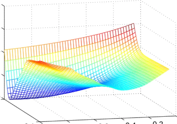
When minimizing S(θ), in the case of a simulated data set, it can be seen that S(θ)may not attain its minimum at the true parameter set but instead at some biased θ. This ’incorrect’ shape ofS(θ)is mainly due to edge effects and dependence between certain parameters. This phenomenon is illustrated in Figure 3.1. It is a plot ofS(θ)as a function of onlyλ andK, wherec and
r are kept fixed at their actual values. Note that we have used the logistic growth function and the area interaction function. It is clear from the graph that S(θ)is decreasing asλmoves away from its actual value0.2.
0 0.2 0.4 0.6 0.8 1 0.05 0.1 0 0.02 0.04 0.06 0.08 λ Plot of S(λ,k,c,r), c = 0.1 and r = 1.5 k S( λ ,k,c,r)
Figure 3.1: Plot ofS(θ)as a function of only λandK. c andrare kept fixed at their actual values, where(λ, K, r, c) = (0.2,0.1,1.5,0.1).
interactions, due to the form of (2.4). In order to control the estimation routine, so that this risk of bias is reduced, the approach of Paper I is to find good starting values,(λ0, K0, c0, r0), (as opposed to arbitrarily chosen ones) and to choose sensible step sizes,δλ,δK,δc,δr. Further details about this fine-tuning
of the optimization can be found in [8].
3.1.2
Estimation of the death and arrival rates
We here give the form of the ML-estimators used for the estimation of α
and µ in Paper I. The estimator µˆ takes the form of the natural death rate function η(·) into consideration, and the α-estimator partially compensates for the unobserved individuals who arrive and die during the same sam-ple interval, (Tk, Tk−1). Note that in Paper I and Paper III, the function
η(Mi(t)) = 1/(1 +Mi(t))is used.
Denote by L1, . . . , LnT the random lifetimes of the nT individuals who have
died from natural causes by time Tn, given some natural death rate function
µη(Mi(t)) (recall that we label an individual i as naturally dead once the
predicted markm˜i(Tj+1;θ, mi(Tj))>0while the actual data individual is alive
at Tj+1, during the calculation of S(θ)). Furthermore, let t0i(L1), . . . , t0i(L
nT)
denote the birth times of the individuals having these lifetimes. Also letTj,i(Lk)
be the last sample time at which individual i(Lk) was observed alive and let
˜
mi(Lk)(Tj,i(Lk)) denote the prediction of its mark at Tj,i(Lk). Furthermore,
under the same natural death rate regime, let S1, . . . , SmT denote the mT
random lifetimes of the individuals who are still alive at timeTnandmi(Sl)(Tn)
the size of each such individual at the final sample time. The (approximate) ML-estimator of the death rate,µ, is given by
ˆ µ = nT , XnT k=1 η m˜i(Lk) Tj,i(Lk) Tj,i(Lk)−t 0 i(Lk) (3.1) + mT X l=1 η(mi(Sl)(Tn)) Tn−t0i(Sl) ! .
Note that the process is observed only at the sampled time points 0 = T0 <
T1 < . . . < Tn = T so that the actual birth times (and death times) of the
individuals remain unknown. Conditioned on the number of individuals ar-riving during (Tj−1, Tj] the arrival times of the individuals will be uniformly
distributed on (Tj−1, Tj) (see e.g. [23]). Thus, when estimating µ, for each
interval (Tj−1, Tj] we simulate as manyU ni(Tj−1, Tj)-distributed birth times
as there are observed newcomers and these are in turn assigned to all individ-uals observed for the first time at Tj. The question regarding which arrival
3.2. Estimation in the ID-process 21 time to assign to which individual is solved by giving the first arrival time to the individual who is the largest at time Tj, the second arrival time to the
individual which is the second largest at time Tj and so forth. This will have
the consequence that the lifetimes will be random. By repeating this procedure a suitable number of times, each time simulating new random birth times, we could generate a set of estimates of µ which are used to estimate a standard error for µˆ. In the case ofη(·)≡1, expression (3.1) reduces to the estimator found in [32]. LetNTj = Sn j=1ΩTj
,j= 1, . . . , n, denote the number of individuals observed at sample times up to Tj. [32] proposes a simple estimator for the arrival
in-tensityα. However, this estimator underestimatesαsince it does not take into account the unobserved individuals who arrive and die within the same sam-ple interval (see [32]). In order to (partially) compensate for these unobserved individuals who arrive and die in the same sample interval, (Tk, Tk−1), when estimating α we use the following estimator (see [8] or the Appendix for its derivation); ˆ α= NTn Tnν(W)+ 1 Tnν(W) n X j=1 NTn ∆Tj−1 Tn 1−e−ˆµη(mi0)∆Tj−1, (3.2)
where bxc denotes the integer part of x, ∆Tj−1 = Tj −Tj−1 and µˆ is the estimate of µfound previously. Note that the first term in expression (3.2) is the estimator found in [32].
3.2
Estimation in the ID-process
We will here look at the estimation of (α, µ)when the ID-process,{N(t)}t≥0, is considered as its own entity. The results presented in this section can be found in Paper II.
Assume now that we sample {N(t)}t≥0 asN1, . . . , Nn at the respective times
0 = T0 < T1 < . . . < Tn. Since the likelihood function for γ = (α, µ) ∈ Γ,
Ln(γ), is given by the joint density of the distribution of(N(T1), . . . , N(Tn)),
by the Markov property ofN(t)it can be factorised into a product of transition probabilities, i.e. Ln(γ) =P(N(T1) =N1)Qnk=2pNk−1Nk(t;γ). By assumption we condition on N(T0) = 0, so that the log-likelihood will be given by
ln(γ) = n X k=1
where∆Tk−1=Tk−Tk−1. In the case of equidistant sampling, i.e. ∆Tk−1=t for eachk= 1, . . . , n, the log-likelihood takes the form
ln(γ) = X i,j∈E
Nn(i, j) logpij(t;γ), (3.4)
whereNn(i, j) =Pnk=11{(Nk−1, Nk) = (i, j)}.
Hereby, for each of the sampling schemes, the likelihood estimator of γ = (α, µ)∈Γ(obtained by replacingNk byN(Tk),k= 0,1, . . ., in the expressions
(3.3) and (3.4)) will be defined as
(ˆαn,µˆn) = ˆγn= arg max
γ∈Γln(γ). (3.5)
3.2.1
The ML-estimators
The ML-estimator forγ= (α, µ)is given by solving the system of equations
( ∂ ∂αln(γ) = P i,j∈ENn(i, j) ∂ ∂αlogpij(t;γ) = 0 ∂ ∂µln(γ) = P i,j∈ENn(i, j)∂µ∂ logpij(t;γ) = 0.
As no closed form solution can be found by solving theses likelihood equations, numerical methods have to be employed in order to get ML-estimates. What is possible, however, is to express the estimator of α as a function of both the sample and the parameter µ, hence reducing the maximisation to a one dimensional problem.
Proposition 3.2.1. The ML-estimator,γˆn= (ˆαn,µˆn), is found by maximising
ln(ˆαn(µ), µ) overΓ2⊆R+ (the projection ofΓ onto the µ-axis), i.e.
ˆ µn = arg max µ∈Γ2 ln(ˆα(µ), µ) ˆ αn = αˆn(ˆµn), where ˆ αn(µ) := µ/(1−e −µt) 21−e−µt µt −e−µt −1 1 n X i,j∈E Nn(i, j)(j−ie−µt) = µ 21−e−µt µt −e−µt −1 1 n e−µtN n−N0 1−e−µt + n X k=0 Nk ! .
3.3. Maximum likelihood inference in the SG-process 23
3.2.2
Asymptotic properties of the ML-estimators
Assume now that we sampleN(t)at the timesTn =nt,n∈N,t >0
(equidis-tant sampling). The following two results show that the ML-estimator (3.5) is strongly consistent (Proposition 3.2.2) and asymptotically Gaussian (Proposi-tion 3.2.3). We denote by γ0 = (α0, µ0) ∈ Γ the true parameter pair of the ID-process. These results can be found in Paper II. For further discussions on ML-estimation in Markov processes and asymptotic properties thereof, see e.g. [2, 4, 11, 18, 35].
Proposition 3.2.2. Let Γ be any compact subset of R2+. Then the maximum
likelihood estimator for the ID-process satisfies
(ˆαn,µˆn) a.s.
−→(α0, µ0)
asn→ ∞, where(α0, µ0)∈Γ is the true parameter pair.
Proposition 3.2.3. Let Γ be any compact subset of R2+. Furthermore,
assume that (log(α0 + µ0) − log(α0))/µ0 ≥ 2t. Then, as n → ∞,
√n((ˆα
n,µˆn)−(α0, µ0))converges in distribution to the two-dimensional
zero-mean Gaussian distribution with covariance matrix, I(γ0)−1, given by
I(γ0)−1= µ0 t((1 + e−µ0t)ρ 0(Ξ−1)−1) (3.6) × ρ0(2τ0−µ0t(1−e−µ0t))+ρ20 µ0t(Ξ−1)(τ0−µ0t) 2 (1−e−µ0t)2 1 + ρ0 µ0t(Ξ−1)(τ0−µ0t) 1 + µ0tρ0(Ξ−1)(τ0−µ0t) µ0t1 (Ξ−1) (1−e−µ0t)2 , where Ξ = Pi,j∈E(pi(j−1)(t;γ0)) 2 pij(t;γ0) πγ0(i), τ0 = 1−e −µ0t −µ0te−µ0t and ρ0 = α0 µ0(1−e −µ0t). Hereπ
γ0(·) =P(P oi(α0/µ0)∈ ·)is the invariant distribution of
the ID-process.
3.3
Maximum likelihood inference in the
SG-process
Conditionally on ΦM(T0) = ΦM(0), assume now that we sample the
SG-process ΦM(t) as φ1, . . . , φn at the sample times T1, . . . , Tn on the
compact region W. Here φk = (1ωk(1)m1k, . . . ,1ωk(N)mdk)
T
, ωk =
{indices of individuals present at timeTk}, k = 1, . . . , n, andd = |Snk=1ωk|.
Now, based on this sampling scheme we want to find the Maximum Likelihood (ML) estimate of the parameter vectorθ= (λ, K, σ, α, µ)∈Θ.
The likelihood function of the parameters of the SG-process, Ln(θ), is given
by the joint density of (ΦM(T1), . . . ,ΦM(Tn)), evaluated at (φ1, . . . , φn) and
treated as a function of θ ∈ Θ. Therefore, depending on whether we choose
Mi(0)to be fixed or drawn from the stationary distribution, we end up
evalu-ating either expression (2.10) or expression (2.11) when we evaluateLn(θ).
3.3.1
ML-estimation:
M
0i
=
M
0∈
R
+When we let all Yi(0) = Mi0 = M0 ∈ R+ be given by the same fixed value, from expression (2.10) we obtain
Ln(θ) =CL1,n(θ)L2,n(θ)L3,n(θ)∝ L1,n(θ)L2,n(θ)L3,n(θ),
where, forki= min{k:i∈ωk},
L1,n(θ) = n Y k=1 Y i∈ωk−1∩ωk pY1(∆Tk, mik|mi(k−1);λ, K, σ) L2,n(θ) = Y i∈Sn k=1ωk 1 ∆Tki Z ∆Tki 0 pY1(t, mi(ki−1)|M0;λ, K, σ)dt L3,n(θ) = n Y k=1 pN ∆Tk,|ωk| |ωk−1|;αν(W), µ .
The (rescaled) log-likelihood is given by
ln(θ) = log C−1Ln(θ)= logL1,n(θ) + logL2,n(θ) + logL3,n(θ)
=: l1,n(θ) +l2,n(θ) +l3,n(θ),
and the ML-estimator ofθ∈Θ, based on(ΦM(T1), . . . ,ΦM(Tn)), will be given
by e θn := θen(ΦM(T1), . . . ,ΦM(Tn)) (3.7) = arg max θ∈Θ ln(θ; ΦM(T1), . . . ,ΦM(Tn)) = arg max θ∈Θ (l1,n(θ) +l2,n(θ) +l3,n(θ)) = θe1,n+eθ2,n = arg max θ∈Θλ×ΘK×Θσ×{0}2 {l1,n(θ) +l2,n(θ)}+ arg max θ∈{0}3×Θ α×Θµ l3,n(θ),
whereby we may estimate the parameters of the ID-process and the parameters related to the mark growth separately. Moreover, since there is no closed form
3.3. Maximum likelihood inference in the SG-process 25 expression available for the ML-estimator (αen,eµn)of the ID-process (see [9]),
there is also no closed form forθen in (3.7). Hence, in modelling situations one
has to rely on numerical methods to findθen.
3.3.2
ML-estimation:
M
0i
∼
π
Under the assumption that we start the diffusions in their stationary distribu-tions,M0
i ∼π, from expression (2.11) we obtain the likelihood function
Ln(θ) =CL1,n(θ)L2,n(θ)∝ L1,n(θ)L2,n(θ)
and the (rescaled) log-likelihood
ln(θ) = log C−1Ln(θ)= logL1,n(θ) + logL2,n(θ)
=: l1,n(θ) +l2,n(θ), where l1,n(θ) = log n Y k=1 Y i∈ωk π(mik;λ, K, σ) ! = n X k=1 X i∈ωk logπ(mik;λ, K, σ) l2,n(θ) = log n Y k=1 pN ∆Tk,|ωk| |ωk−1|;αν(W), µ ! = n X k=1 logpN ∆Tk,|ωk| |ωk−1|;αν(W), µ .
Here, just as in the fixed initial value case of Section 3.3.1, we deal with the separate estimators ˆ θn = θˆ1,n+ ˆθ2,n= arg max θ∈Θλ×ΘK×Θσ×{0}2 l1,n(θ) + arg max θ∈{0}3×Θ α×Θµ l2,n(θ)(3.8)
and, similarly, there is no closed form expression available forθˆn.
3.3.3
Asymptotic inference under stationarity
When dealing with asymptotic spatial statistics, there are different types of asymptotics which may be considered. In the case of the SG-process, within the framework of so called increasing domain asymptotics (see e.g. [39]), there essentially are two different ways to increase the total number of individuals
considered, and consequently also the number of transitions taking place be-tween pairs of consecutive sample timesTk−1andTk; Either increase the
num-ber of sample points or increase the size ofW. We here consider the approach where we increase the number of sample times, i.e. we apply the equidistant sampling schemeTk =k∆, k= 1, . . . , n,∆>0, where T =Tn =n∆. We will
denote byθ0= (λ0, K0, σ0, α0, µ0)∈Θthe true parameter vector value which generatesΦM, and we assume thatΘis a subset of R5+ such that
Θ∩ {(λ, K, σ, α, µ)∈R5
+: 2λ < σ2}=∅. (3.9) Recall that this is required to keep theYi(t)’s positive.
Theorem 3.3.1 (Consistency). Let Θ be a compact subset of R5+ such that
(3.9) holds. Then, forθ0∈Θ, the estimator θˆn in expression (3.8) is strongly
consistent, i.e. as n→ ∞,
ˆ
θn a.s.
−→θ0.
Now, by putting some additional restrictions on the parameters we may also prove the following theorem.
Theorem 3.3.2(Asymptotic normality). Let θ0be in the interior ofΘ, where
Θis a compact subset ofR5+such that (3.9) holds. Require further that θ0 and
∆>0 are such that (log(α0+µ0)−log(α0))/µ0≥2∆.
Assume thatλ0is known, so thatθˆn= ( ˆKn,σˆn,αˆn,µˆn)is the ML-estimator of
θ0= (K0, σ0, α0, µ0). Then, asn→ ∞, we obtain √ n θˆn−θ0−→d Y∼N 04×1, µ0 α0 K2 0σ 2 0 2λ0 0 01×2 0 µ0α0 σ40 8λ0C(θ0) 01×2 02×1 02×1 IN(θ0)−1 , where C(θ) = σ2λ2ψ0 2σλ2 −1 > 0, ψ(x) = Γ0(x)/Γ(x), 0i×j denotes the i×j
zero matrix and the 2×2 matrixIN(θ0)−1, which can be found in expression
(3.6), is the covariance matrix related to the ID-process.
Similarly, when σ0 is known, we estimate θ0 = (λ0, K0, α0, µ0) by θˆn =
(ˆλn,Kˆn,αˆn,µˆn)and, as n→ ∞, we obtain √ n θˆn−θ0 d −→Y∼N 04×1, µ0 α0 λ0σ2 0 2C(θ0) 0 01×2 0 µ0α0K02σ 2 0 2λ0 01×2 02×1 02×1 IN(θ0)−1 .
3.4. Spatio-temporal edge correction 27
3.4
Spatio-temporal edge correction
When sampling real data, {X(Tk)}nk=1, one usually considers all individuals
within some regionA(in Figure 1.1 circular) which is part of some larger region
W. The individuals inAinteract with each other but simultaneously also with the individuals present outsideA, i.e. the individuals inB=W\A. So, if one were to estimate some statistics and/or model parameters in a situation where the interaction among (neighbouring) individuals plays a role, by only taking into consideration the individuals in A the estimators may generate biased estimates since the interaction between the individuals in A and those in B
would be neglected. The effects of the absence of the information regarding this interaction are commonly referred to asedge effects. The risk that the edge effects generate biases rapidly increases when one deals with small quantities of data in A, as is the case with our tree data set introduced in Figure 1.1. Hence, some type of correction method is needed (see e.g. [12, 20, 38]). We here give the idea behind the edge correction methods proposed in Pa-per I. One starts by finding initial (possibly biased) estimates of the model parameters, θˆ∗, based on the original data set (region A). Then, under the regime ofθˆ∗, we wish to find the expected model behaviour when restricted to region B (possibly conditioned on the actual data inA), Eˆ
θ∗[ΦM[0, T]|B]. By doing so we wish to establish the expected interaction between the individuals in B and the individuals in region A. With Eˆ
θ∗[ΦM[0, T]|B] at hand we now re-estimate the model parameters from the actual data (region A), however, this time allowing forEˆ
θ∗[ΦM[0, T]|B]to interact with the actual data during the estimation. Once these new estimates have been obtained, we let them replace θˆ∗ and repeat the above procedure again. By continuing in this fash-ion we have an iterative procedure which we stop once it has fulfilled a given predefined convergence criterion.
The three edge correction methods presented in Paper I. We refer to as them as The simple correction method, The rotated surrounding correction method
and The influenced growth correction method, and they are all explained for the GI-process but they may be applied to other spatial and spatio-temporal (marked) point processes as well. In the algorithms presented in Paper I the large rectangular window W will be wrapped onto a torus when we generate the individuals in the outer region,B, (see e.g. [12, 25, 29, 38]).
Chapter 4
Future work and extensions
There are some remarks which may be addressed about the general development of the GI-process. Note that the GI-process here is presented for a single species. However, it can easily be extended to include the scenario where interaction takes place also between different species, living and interacting within the same study region. This extension is made by letting each species be governed by both its unique open-growth function and interaction function, and the latter can be different within and between species. Hereby the amount an individual is affected by its neighbours not only depends on its distance to the neighbours and the neighbours’ sizes, but also on the species of the neighbours.
An improvement of Paper II that possibly can be made is to improve the in-vertibility condition given in Proposition 3.2.3 in Chapter 3 so that asymptotic normality holds for all (α0, µ0) ∈ Θ. Furthermore, in order to become more realistic in applications,N(t)could be extended by letting the arrival intensity,
α, and the death rate,µ, be non-constant functions of time, or in themselves Markov chains (in the latter caseN(t)thus becomes a hidden Markov model). Results similar to the ones found in Paper II could be established and the type of modelling done in Paper I could be developed.
Regarding the development of Paper IV, we could employ some other positive diffusion for the growth of the marks. It should be noted that the linear growth function, which is the drift function in the CIR-process, is a special case of the Richards growth function (see e.g. [28, 31]). Hence, a further possibility would be to use the Richards growth function, or one of its other special cases, as drift in the mark-SDEs dYi(t).
A further modification which may be made is to change the diffusion term
σ(Yi(t);θ) =σ p
Yi(t)into any other diffusion term which keepsYi(t)positive,
e.g. σ(Yi(t);θ) = σYi(t)γ, γ > 0, which is the diffusion coefficient found in
the CKLS-model (see e.g. [5]). Note that when applying these changes, we would typically not have known closed form expressions for the transition den-sities,pYi(t, y1|y0;θ). The transition densities are know only for a few special
cases, including the CIR-process. Therefore, we have to use different approx-imated/pseudo likelihood methods for the estimation of the parameters (see [19] for a good general overview).
Our final goal is to ML-estimate all parameters of the full SGI-process, i.e. to include also the spatial interaction function h(·) in the SDEs. Note that on a compact space-time domain this amounts to considering a multivariate diffusion. Here the lack of closed form expression for the transition densities remains and, just as for the previous adjustments suggested, the estimation re-quires that we employ approximated/pseudo likelihood methods. For instance, [1] suggests an approach where the transition densities of multivariate diffusions may be approximated by series expansions based on hermite polynomials. Note further that within this setting, in order to reduce edge effects (absence of in-dividuals outside the boundary ofW), it would be sensible to choose W to be a torus. Furthermore, instead of using the edge correction methods in Paper I, an altered version could be considered which is more in the lines of an EM-algorithm. This would also allow us to study convergence properties of the edge corrected ML-estimators of the SGI-process from a theoretical perspective. Thus far we have introduced only natural deaths in the SG(I)-process. It should be possible also to introduce competitive deaths as well, however, this would entail a slightly different formulation of the diffusionsMi(t),i= 1, . . . , N. By
defining the death-time of individualito be (the stopping-time) ζi = inf{t >
Bi:Mi(t) = 0}∧Di, it follows that ifMireaches the absorbing stateMi(t) = 0
for some t∈ (Bi, Di), where Di =Bi+Li, it stays 0 and we say that it has
suffered a competitive death. Furthermore, if it does not die from competition during(Bi, Di)it will still die at timeDi, i.e. at its natural death time. As soon
as t > ζi the interaction between Mi(t) and the other marks will terminate,
hence we remove individualifrom consideration.
Paper I motivated the study conducted in Paper III. Although the modifica-tions of the GI-process made in Paper III improved the fit to the Scots pine data type considered, some improvements can still be made. It was seen that spatial characteristics and basal area of simulated predictions were similar to the ones of the data. However, it was also seen that the empirical diameter distributions of the data trees and the simulated predicted trees differed, and we further also saw that the predicted and observed number of alive individuals differed
sub-31 stantially. The former seems to be the result of the chosen growth/interaction functions, whereas the latter seems to be the result of having only very few (3) sample time points to estimate the ID-process. Hence, although the GI-process described the data quite well in most aspects, there are still improvements to be made. As a first step one should try to fit the model to data sets with more observed time points. A further step which could be made is to evaluate other kinds of growth and interaction functions to see if the fit is improved. It is also our belief that once we have developed the ML-estimation scheme for the SGI-process (with interaction), a better approach to fitting the process to data will be available. We further hope that this could improve the modelling of the considered (pine) stands.