Rowan University Rowan University
Rowan Digital Works
Rowan Digital Works
Theses and Dissertations
9-2-2014
Optimization algorithms for inference and classification of
Optimization algorithms for inference and classification of
genetic profiles from undersampled measurements
genetic profiles from undersampled measurements
Belhassen BayarFollow this and additional works at: https://rdw.rowan.edu/etd
Part of the Electrical and Computer Engineering Commons
Let us know how access to this document benefits you -
share your thoughts on our feedback form.
Recommended Citation Recommended Citation
Bayar, Belhassen, "Optimization algorithms for inference and classification of genetic profiles from undersampled measurements" (2014). Theses and Dissertations. 410.
OPTIMIZATION ALGORITHMS FOR INFERENCE AND CLASSIFICATION OF GENETIC PROFILES FROM
UNDERSAMPLED MEASUREMENTS
by
Belhassen Bayar
A Thesis Submitted to the
Department of Electrical & Computer Engineering College of Engineering
In partial fulfillment of the requirement For the degree of
Master of Science at
Rowan University June 2014
ACKNOWLEDGEMENTS
I want to express my sincere gratitude to Dr. Nidhal Bouaynaya, my supervisor who has always bothered to offer me the best working conditions possible. I thank her for her wide availability, her high scientific qualifications and her guidance, illuminating discussions related to this work and beyond, encouragement, moral and financial support in this research.
I express my appreciation and gratitude to Dr. Roman Shterenberg , Associate Professor at the University of Alabama at Birmingham USA, for the time he spent with me, his availability even when he was abroad and the valuable advice he has given me throughout my research.
I also would like to express my deep and sincere gratitude to Dr. Robi Polikar, Professor & Chair at the ECE Department, for the high quality courses he teaches, his availability and eagerness to provide the best learning experience for students at the department.
Many thanks to all the students who accompanied me during these years and have continued to create a good working atmosphere within the laboratory. Deepest thanks to my dear parents and grandmother to whom I owe so much. I would have neither the means nor the strength to accomplish this work without them. I also want to express my gratitude to my friends who have continued to give me the moral and intellectual support throughout my work during all the good and bad moments. They always say the best is for the end, that’s why I dedicate this project to my dear sister, my little light that gave me energy and courage.
Abstract
Belhassen Bayar
OPTIMIZATION ALGORITHMS FOR INFERENCE AND CLASSIFICATION OF GENETIC PROFILES FROM UNDERSAMPLED MEASUREMENTS
2014/06
Nidhal Bouaynaya, Ph.D.
Master of Science in Electrical & Computer Engineering
In this thesis, we tackle three different problems, all related to optimization tech-niques for inference and classification of genetic profiles. First, we extend the de-terministic Non-negative Matrix Factorization (NMF) framework to the probabilistic case (PNMF). We apply the PNMF algorithm to cluster and classify DNA microar-rays data. The proposed PNMF is shown to outperform the deterministic NMF and the sparse NMF algorithms in clustering stability and classification accuracy. Sec-ond, we propose SMURC: Small-sample MUltivariate Regression with Covariance estimation. Specifically, we consider a high dimension low sample-size multivariate regression problem that accounts for correlation of the response variables. We show that, in this case, the maximum likelihood approach is senseless because the likeli-hood diverges. We propose a normalization of the likelilikeli-hood function that guaran-tees convergence. Simulation results show that SMURC outperforms the regularized likelihood estimator with known covariance matrix and the state-of-the-art sparse Conditional Graphical Gaussian Model (sCGGM). In the third Chapter, we derive a
new greedy algorithm that provides an exact sparse solution of the combinatorial `0
Table of Contents
List of Figures vii
List of Tables viii
1 Introduction 1
1.1 Research Objectives 1
1.2 Research Contribution 1
1.3 Organization 2
2 PNMF: Theory & Application To Microarray Data Analysis 4
2.1 Introduction 4
2.2 Non-negative Matrix Factorization 10
2.3 Probabilistic Non-negative Matrix Factorization 13
2.4 PNMF-based Data Classification 15
2.5 Application to Gene Microarrays 19
2.6 Conclusion and Discussion 34
3 High-Dimension SMURC Estimation 36
3.1 Introduction 36
3.2 The Normalized-Likelihood 41
3.3 Application: Genetic Regulatory Networks 53
4 Kernel Reconstruction V.S. `0-based CS 62 4.1 Introduction 62 4.2 Compressed Sensing 63 4.3 Kernel Reconstruction 76 4.4 Conclusion 79 Bibliography 80 A Appendix 86
List of Figures
2.1 Clustering results for the Leukemia dataset 20
2.2 Metagenes expression patterns versus the samples for k= 4 21
2.3 Clustering results for the Medulloblastoma dataset 22
2.4 Clustering Percentage Error versus Nbr. of genes 28
2.5 The cophenetic coefficient versus the standard deviation 29
2.6 Cophenetic versus SNR in dB in Leukemia dataset 30
2.7 Cophenetic versus SNR in dB in Medulloblastoma dataset 31
3.1 Approximation of the optimization problem in Proposition 4 49
3.2 Approximation error||S−S ∗ ||F/||S||F versus n 51
3.3 Performance comparison of SMURC with sCGGM and RMLE 53
3.4 The known undirected gene interactions in the Drosophila 57
3.5 Estimated gene regulatory networks of the Drosophila 57
4.1 Performance comparison of KR with`1-based and`2-based CS forN = 10 78
List of Tables
2.1 Smallest SNR value for ρ≥0.9 32
2.2 Classification accuracy 34
Chapter 1 Introduction
1.1 Research Objectives
We outline the goal of this research through the following objectives:
1. Study and analyse the Non-negative Matrix Factorization (NMF) and propose a probabilistic extension to NMF (PNMF) for data corrupted by noise.
2. Build a PNMF-based classifier and apply it for tumor classification from gene expression data.
3. Derive a convex optimization algorithm for the solution of an under-determined multivariate regression problem. Apply the proposed algorithm to infer genetic regulatory networks from gene expression data.
4. Derive a greedy algorithm for exact reconstruction of sparse signals from a limited number of observations.
1.2 Research Contribution
This work contributes to the field of computational bioinformatics and biology through the application of the signal processing algorithms aiming to study and analyze the microarray data. Our work shifts the focus of the genomic signal processing commu-nity from analyzing the genes expression patterns and samples clusters to considering
the mathematical aspect of the algorithm and deriving its application in the stochas-tic work. We also focus on solving under-determined multivariate regression systems in order to infer gene regulatory networks. These networks are known to be sparse, therefore, we have a great interest in studying the compressive sensing approach which recovers sparse signal from linear model. Specific contributions of this work include:
The improvement of the mathematical proof for the NMF algorithm by
provid-ing a general evidence (see Appendix preposition 2).
The development of a new NMF algorithm for the noisy Microarray data in
order to improve the basic NMF approach and to predict some hidden data features.
Solving under-determined multivariate regression systems to infer gene
regula-tory networks using our new SMURC algorithm.
Recover k-sparse signal using our new approach, called Kernel Reconstruction,
that guarantees an exact reconstruction and less computational time comparing
to the `0-based compressive sensing approach [18].
1.3 Organization
This thesis is organized as follows.
In Chapter 2, we study and analyze the Non-negative Matrix Factorization and de-rive its probabilistic approach that we call PNMF algorithm and then we dede-rive its
the Appendix chapter. We compare the performance of our PNMF approach with its homologues in clustering as well as classification.
In Chapter 3, we develop a new approach, called Small-sample MUltivariate Re-gression with Covariance Estimation (SMURC), to solve under-determined multivari-ate regression systems. We use this approach to infer gene regulatory networks. We compare our algorithm to other techniques cited in related works and using a syn-thetic data. Subsequently, we apply our approach to infer the know interactions in the Drosophila’s 11-gene wing muscle network.
Finally, in Chapter 4 we provide a complete review of the compressive sensing technique. We also come up with a new approach that performs an exact reconstruc-tion of a sparse signal. We call this approach, Kernel Reconstrucreconstruc-tion, and we compare it with what has been suggested in the related work.
Chapter 2
Probabilistic Non-negative Matrix Factorization: Theory and Application to Microarray Data Analysis
2.1 Introduction
Extracting knowledge from experimental raw data and measurements is an important objective and challenge in signal processing. Often data collected is high dimensional and incorporates several inter-related variables, which are combinations of underly-ing latent components or factors. Approximate low-rank matrix factorizations play a fundamental role in extracting these latent components [14]. In many applica-tions, signals to be analyzed are non-negative, e.g., pixel values in image processing, price variables in economics and gene expression levels in computational biology. For such data, it is imperative to take the non-negativity constraint into account in or-der to obtain a meaningful physical interpretation. Classical decomposition tools, such as Principal Component Analysis (PCA), Singular Value Decomposition (SVD), Blind Source Separation (BSS) and related methods do not guarantee to maintain the non-negativity constraint. Non-negative matrix factorization (NMF) represents non-negative data in terms of lower-rank non-negative factors. NMF proved to be
such as muscle identification in the nervous system [54], classification of images [29], gene expression classification [10], biological process identification [32] and transcrip-tional regulatory network inference [38]. The appeal of NMF, compared to other clustering and classification methods, stems from the fact that it does not impose
any prior structure or knowledge on the data. Brunet et al. successfully applied
NMF to the classification of gene expression datasets [10] and showed that it leads to more accurate and more robust clustering than the Self-Organizing Maps (SOMs) and Hierarchical Clustering (HC). Analytically, the NMF method factors the original
non-negative matrixV into two lower rank non-negative matrices,W andH such that
V =W H+E, whereE is the residual error. Lee and Seung [33] derived algorithms
for estimating the optimal non-negative factors that minimize the Euclidean distance and the Kullback-Leibler divergence cost functions. Their algorithms, guaranteed to converge, are based on multiplicative update rules, and are a good compromise be-tween speed and ease of implementation. In particular, the Euclidean distance NMF algorithm can be shown to reduce to the gradient descent algorithm for a specific choice of the step size [33]. Lee and Seung’s NMF factorization algorithms have been widely adopted by the community [6, 10, 19, 59].
The NMF method is, however, deterministic. That is, the algorithm does not take into account the measurement or observation noise in the data. On the other hand, data collected using electronic or biomedical devices, such as gene expression profiles, are known to be inherently noisy and therefore, must be processed and analyzed by systems that take into account the stochastic nature of the data. Furthermore, the ef-fect of the data noise on the NMF method in terms of convergence and robustness has
not been previously investigated. Thus, questions about the efficiency and robustness of the method in dealing with imperfect or noisy data are still unanswered.
In this chapter, we extend the NMF framework and algorithms to the stochastic case, where the data is assumed to be drawn from a multinomial probability den-sity function. We call the new framework Probabilistic NMF or PNMF. We show that the PNMF formulation reduces to a weighted regularized matrix factorization problem. We generalize and extend Lee and Seung’s algorithm to the stochastic case; thus providing PNMF updates rules, which are guaranteed to converge to the optimal solution. The proposed PNMF algorithm is applied to cluster and classify gene ex-pression datasets, and is compared to other NMF and non-NMF approaches including sparse NMF (SNMF) and SVM.
The chapter is organized as follows: In Section 2.1.1, we discuss related work and clarify the similarities and differences between the proposed PNMF algorithm and other approaches to NMF present in the literature. In Section 2.2, we review the (deterministic) NMF formulation and extend Lee and Seung’s NMF algorithm to include a general class of convergent update rules. In Section 2.3, we introduce the probabilistic NMF (PNMF) framework and derive its corresponding update rules. In Section 2.4, we present a data classification method based on the PNMF algorithm. Section 2.5 applies the proposed PNMF algorithm to cluster and classify gene ex-pression profiles. The results are compared with the deterministic NMF, sparse NMF and SVM. Finally, a summary of the main contributions and concluding remarks are
denoted by bold lower case letters, e.g., x,y; and matrices are referred to by upper
case letters, e.g., A, V. xi denotes the ith element of vector x and Aij is the (i, j)th
entry of matrix A. Throughout the chapter, we provide references to known results
and limit the presentation of proofs to new contributions. All proofs are presented in the Appendix section.
2.1.1 Related work. Several variants of the NMF algorithm have been pro-posed in the literature. An early form of NMF, called Probabilistic Latent Semantic Analysis (PLSA) [27], [28], [37], was used to cluster textual documents. The key idea is to map high-dimensional count vectors, such as the ones arising in text documents,
to a lower dimensional representation in a so-called latent semantic space. PLSA
has been shown to be equivalent to NMF factorization with Kullback-Leibler (KL) divergence, in the sense that they have the same objective function and any solution of PLSA is a solution of NMF with KL minimization [17].
Many variants of the NMF framework introduce additional constraints on the
non-negative factor matrices W and H, such as sparsity and smoothness.
Combin-ing sparsity with non-negative matrix factorization is partly motivated by modelCombin-ing neural information processing, where the goal is to find a decomposition in which the hidden components are sparse. Hoyer [30] combined sparse coding and non-negative
matrix factorization into non-negative sparse coding (NNSC) to control the
trade-off between sparseness and accuracy of the factorization. The sparsity constraint is
negative values of one of the factor matrices to zero. This procedure is not always guaranteed to converge to a stationary point. Kim and Park [31] solved the sparse NMF optimization problem via alternating non-negativity-constrained least squares. They applied sparse NMF to cancer class discovery and gene expression data analysis. NMF has also been extended to consider a class of smoothness constraints on the optimization problem [41]. Enforcing smoothness on the factor matrices is desirable in applications such as unmixing spectral reflectance data for space object identification and classification purposes [41]. However, the algorithm in [41] forces positive entries by setting negative values to zero and hence may suffer from convergence issues. Similarly, different penalty terms may be used depending upon the desired effects on the factorization. A unified model of constrained NMF, called versatile sparse matrix factorization (VSMF), has been proposed in [34]. The VSMF framework includes
bothl1 and l2-norms. Thel1-norm is used to induce sparsity and the l2-norm is used
to obtain smooth results. In particular, the standard NMF, sparse NMF [30], [31] and semi-NMF [16], where the non-negativity constraint is imposed on only one of the factors, can be seen as special cases of VSMF.
Another variant of the NMF framework is obtained by considering different dis-tances or measures between the original data matrix and its non-negative factors [49], [56]. Sandler and Lindenbaum [49] proposed to factorize the data using the earth movers distance (EMD). The EMD NMF algorithm finds the local minimum by solv-ing a sequence of linear programmsolv-ing problems. Though the algorithm has shown
have proposed the wavelet-based approximation to the EMD distance, WEMD, and used it in place of EMD. They argued that the local minima of EMD and WEMD are generally collocated when using a gradient-based method. A similarity measure based on the correntropy, termed NMF MCC, has been proposed in [56]. The correntropy measure employs the Gaussian kernel to map the linear data space to a non-linear space. The optimization problem is solved using an expectation maximization based approach.
A collection of non-negative matrix factorization algorithms implemented for
Mat-lab is avaiMat-lable at http://cogsys.imm.dtu.dk/toolbox/nmf/. Except for PLSA,
which was originally proposed as a statistical technique for text clustering, the pre-sented NMF approaches do not explicitly assume a stochastic framework for the data. In other words, the data is assumed to be deterministic. In this work, we assume that the original data is a sample drawn from a multinomial distribution and derive the maximum a posteriori (MAP) estimates of the non-negative factors. The proposed NMF framework, termed Probabilistic NMF or PNMF, does not impose any addi-tional constraints on the non-negative factors like SNMF or VSMF. Interestingly, however, the formulation of the MAP estimates reduces to a weighted regularized matrix factorization problem that resembles the formulations in constrained NMF approaches. The weighting parameters, however, have a different interpretation: they refer to signal to noise ratios rather than specific constraints.
2.2 Non-negative Matrix Factorization
The non-negative matrix factorization (NMF) is a constrained matrix factorization
problem, where a non-negative matrixV is factorized into two non-negative matrices
W andH. Here, non-negativity refers to elementwise non-negativity, i.e., all elements
of the factors W and H must be equal to or greater than zero. The non-negativity
constraint makes NMF more difficult algorithmically than classical matrix factoriza-tion techniques, such as principal component analysis and singular value decompo-sition. Mathematically, the problem is formulated as follows: Given a non-negative
matrix V ∈ Rn×m, find non-negative matrices W ∈
Rn×k and H ∈ Rk×m such that
V ≈ W H. The optimal factors minimize the squared error and are solutions to the
following constrained optimization problem,
(W∗, H∗) = arg min
W,H≥0
f(W, H) = kV −W Hk2F, (2.1)
where k.kF denotes the Frobenius norm and f is the squared Euclidean distance
function between V and W H. The cost function f is convex with respect to either
the elements of W or H, but not both. Alternating minimization of such a cost
leads to the ALS (Alternating Least squares) algorithm [25], [55], [1], which can be described as follows:
1. Initialize W randomly or by using any a priori knowledge.
4. estimate W as W =V HT(HHT)− with fixed H.
5. Set all negative elements of W to zero or some small positive value.
In this algorithm, A− denotes the Moore-Penrose inverse of A. The ALS algorithm
has been used extensively in the literature [25], [55], [1]. However, it is not guaranteed to converge to a global minimum nor even a stationary point. Moreover, it is often not sufficiently accurate, and it can be slow when the factor matrices are ill-conditioned or when the columns of these matrices are co-linear. Furthermore, the complexity of the ALS algorithm can be high for large-scale problems as it involves inverting a large matrix. Lee and Seung [33] proposed a multiplicative update rule, which is proven to converge to a stationary point, and does not suffer from the ALS drawbacks. In what follows, we present Lee and Seung’s multiplicative update rule as a special case of a class of update rules, which converge towards a stationary point of the NMF problem.
Proposition 1. The function f(W, H) =kV −W Hk2F is non-increasing under the update rules hk+1 =hk−Kh−1(WTWhk −WTv) ˜ wk+1 = ˜wk−K−1 w (HHTw˜k−Hv˜) (2.2)
where w˜ and v˜ are the columns of WT and VT, respectively, and Kh and Kw
satisfy the following conditions
a. Kh and Kw are diagonal matrices with (strictly) positive elements for all vectors
b. Khhk≥WTWhk and Kww˜k≥HHTw˜k where the inequality is elementwise.
c. The matrices Kh−WTW and Kw−HHT are positive semi-definite (p.s.d) for all
h and w˜.
The function f is invariant under these update rules if and only if W and H are at a stationary point.
The following corollary presents a special choice of the matricesKh andKw, which
leads to Lee and Seung’s multiplicative rule for the NMF problem.
Corollary 2.2.1. In Proposition 1, chose Kh and Kw as follows:
(Kh)ij =δij(WTWhk)i/hki, (2.3)
(Kw)ij =δij(HHTw˜k)i/w˜ki, (2.4)
Where hki,w˜ki are the ith entries of the vectors hk and w˜k, respectively, andδ
ij is the
kronecker function, i.e., δij = 1, if i=j 0, otherwise.
This choice leads to the following update rule: Hij ←− Hij (WTV) ij (WTW H) ij Wij ←− Wij (V HT) ij (W HHT) ij (2.5)
The function f is invariant under these updates if and only if W and H are at a stationary point.
ary point of the NMF problem. From the proof of the Proposition (detailed in the Appendix), it will be clear that conditions [a], [b] and [c] in Proposition 1 are only sufficient conditions for the update rules to converge towards a stationary point. That
is, there may exist Kh and Kw that do not satisfy these conditions but that lead to
update rules that converge towards a stationary point. The particular choice of Kh
and Kw in Corollary 1 corresponds to the fastest convergent update rule among all
matrices satisfying conditions [a]-[c] in Proposition 1. Observe also that since the
data matrix V is non-negative, the update rule in (2.5) leads to non-negative factors
W and H as long as the initial values of the algorithm are chosen to be non-negative.
2.3 Probabilistic Non-negative Matrix Factorization
2.3.1 The PNMF framework. In this section, we assume that the data,
represented by the non-negative matrix V, is corrupted by additive white Gaussian
noise. Then, the data follows the following conditional distribution,
p(V |W, H, σ2) = N Y i=1 M Y j=1 [N(Vij |uTi hj, σ2)], (2.6)
whereN(.|µ, σ2) is the probability density function of the Gaussian distribution with
mean µ and standard deviation σ, ui and hj denote, respectively, the ith column of
the matrix U =WT (or theith row ofW) and the jth column of the matrix H. Zero
Specifically, we have p(U |σ2W) = N Y i=1 N(ui |0, σ2WI) = p(W |σ 2 W). (2.7) p(H |σH2) = M Y i=1 N(hj |0, σH2I). (2.8)
We estimate the factor matrices W and H using the maximum a posteriori (MAP)
criterion. The logarithm of the posterior distribution is given by
ln(p(W, H |V, σ2, σH2 , σW2 )) =− 1 2σ2 N X i=1 M X j=1 (Vij −uTi hj)2 − 1 2σ2 W N X i=1 kuik2− 1 2σ2 H M X j=1 khjk2+C, (2.9)
whereC is a constant term depending only on the standard deviationsσ, σW andσH.
Maximizing (2.9) is equivalent to minimizing the following function
(W∗, H∗) = arg min W,H≥0 k V −W Hk2F +λWkWk2F + λHkHk2F, (2.10) where λW = σ 2 σ2 W and λH = σ 2 σ2 H
. Observe that the PNMF formulation in (2.10)
corresponds to a weighted regularized matrix factorization problem. Moreover, the
PNMF reduces to the NMF forσ = 0. The following proposition provides the update
Proposition 2. The function
f(W, H) =kV −W Hk2F +αkWk2F +βkHk2F (2.11)
is non-increasing under the update rules
Hij ←− Hij (WTV) ij (WTW H+βH) ij Wij ←− Wij (V HT) ij (W HHT+αW) ij (2.12)
The function f is invariant under these updates if and only if W and H are at a stationary point.
Observe that, since the data matrix V is non-negative, the update rules in (2.12)
lead to non-negative factors W and H as long as the initial values of the algorithm
are chosen to be non-negative.
2.4 PNMF-based Data Classification
In this section, we show how the PNMF output can be used to extract relevant features from the data for classification purposes. The main idea relies on the fact that metasamples extracted from the PNMF factorization contain the inherent structural information of the original data in the training set. Thus, each sample in a test set can be written as a sparse linear combination of the metasamples extracted from the training set. The classification task then reduces to computing the representation coefficients for each test sample based on a chosen discriminating function. The
sparse representation approach has been shown to lead to more accurate and robust
results [64]. The sparsity constraint is imposed through anl1-regularization term [64].
Thus, a test sample may be represented in terms of few metasamples.
2.4.1 Sparse Representation Approach. We divide the data, represented
by the n×m matrix V, into training and testing sets, where the number of classesk
is assumed to be known. In Section 2.5, we describe a method to estimate the number of classes based on the PNMF clustering technique. The training data is ordered into
a matrix A with n rows of genes and r columns of training samples with r < m.
Thus, A is a sub-matrix of V used to recognize any new presented sample from the
testing set. We arrange the matrix A in such a way to group samples which belong to
the same class in the same sub-matrix Ai where (1≤i≤k). Then A can be written
asA= [A1, A2, ...., Ak] and each matrix Ai is a concatenation of ri columns of theith class Ai = [ci,1,ci,2, ....,ci,ri]
A test sample y∈Rn that belongs to theith class can be written as the following
linear combination of the Ai columns,
y=αi,1ci,1+αi,2ci,2+...+αi,rici,ri, (2.13)
for some scalars αi,q∈R, 1≤q≤ri.
y=Ax, (2.14)
where
x= [0, ...0, αi,1, αi,2, ..., αi,ri,0...,0]
T
∈Rr, (2.15)
is the coefficient vector of the testing sampley. xis ari-sparse vector whose nonzero
entries are associated with the columns of the sub-matrix Ai, hence the namesparse
representation. Therefore, predicting the class of test sampley reduces to estimating
the vector x in Eq. (2.14).
We propose to find the sparsest least-squares estimate of the coefficient x as the
solution to the following regularized least-squares problem [57]
ˆ
x= min
x {kAx−yk2+λkxk1}, (2.16)
where kxk1 denotes the l1-norm of vector x, i.e., kxk1 =
P
i|xi|, and λ is a positive
scalar used to control the tradeoff between the sparsity of x and the accuracy of
the reconstruction error. Donoho et al. showed that the l1-norm approximates the
l0-norm, which counts the number of non-zero entries in a vector [18]. The l0-norm
problem, however, is NP hard, whereas the l1-norm is convex. The optimization
problem in (2.16) is therefore convex; thus, it admits a global solution, which can be efficiently computed using convex optimization solvers [23]. Actually, one can show that (2.16) is a Second-Order Cone Programming (SOCP) problem [9].
2.4.2 PNMF-based classification . The classifier’s features are given by the metasamples computed by the PNMF algorithm. We first compute the PNMF
factorization of each sub-matrix Ai as
Ai ∼Wi×Hi, (2.17)
whereWi andHi are respectivelyn×ki and ki×ri non-negative matrices. ki refers to
the number of metasamples needed to describe and summarize theithclass. The value
of ki is experimentally determined and depends on the number of training samples
ri in each class and the total number of classes k. We subsequently concatenate all
the Wi matrices to form the matrix W = [W1, W2, .., Wk]. Observe that the matrix
W contains the metasamples of the entire training set. Therefore, a test sample y
that belongs to the ith class should approximately lie in the space spanned by theW
i columns.
The classification problem in (2.16) can therefore be re-written as
ˆ
x= min
x {kWx−yk2+λkxk1}, (2.18)
Which can be easily solved using a SOCP solver [9].
PNMF-based classification algorithm The PNMF-based classification algorithm is summarized below.
Input: Gene expression data V ∈ Rn×m. It is assumed that V contains at least r labeled samples, which can be used in the learning or training process.
Step 1 Select the training samples A∈Rn×r and the testing sample y ∈
Rn from
the original data V such thaty is not a column of A.
Step 2 Reorder the training matrix A= [A1, A2, ..., Ak] for k classes.
Step 3 Compute the matrix of featuresWi ∈Rn×kifrom each sub matrixAi ∈Rn×ri
Using the PNMF algorithm, i= 1 :k
Step 4 Solve the optimization problem in (2.18) for
W = [W1, W2, ..., Wk] using, for instance, the cvx environment in MATLAB. Let the solution x= [xT1,· · · ,xTk]T, where xi ∈Rki×1.
Step 5 Compute the residuals ei(y) = ky−W δi(x)k2, i = 1 : k, where δi(x) = [0,· · · ,0,xT
i ,0,· · ·0]T .
Step 6 Associate class(y)=arg miniei(y)
2.5 Application to Gene Microarrays
We apply and compare the proposed PNMF-based clustering and classification al-gorithms with its homologue NMF-based clustering [10] and classification as well as
Samples Samples K=2 5 10 15 20 25 30 35 10 20 30 5 10 15 20 25 30 35 10 20 30 5 10 15 20 25 30 35 10 20 30 K=3 5 10 15 20 25 30 35 10 20 30 5 10 15 20 25 30 35 10 20 30 5 10 15 20 25 30 35 10 20 30 K=4 5 10 15 20 25 30 35 10 20 30 5 10 15 20 25 30 35 10 20 30 5 10 15 20 25 30 35 10 20 30 0 0.2 0.4 0.6 0.8 1 (a) 2 3 4 5 6 0.8 0.82 0.84 0.86 0.88 0.9 0.92 0.94 0.96 0.98 1 Rank K Cophenetic Coefficient ρ
Cophenetic coefficient versus Rank K
PNMF NMF−Euc NMF−Div
(b)
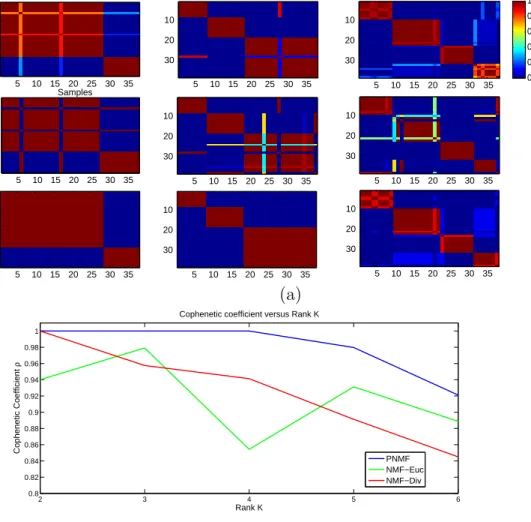
Figure 2.1: Clustering results for the Leukemia dataset: (a) Consensus matrices: Top row NMF-Euc, Second row NMF-Div, bottom row: PNMF; (b) Cophenetic coefficient
1 3 5 7 9 11 13 15 17 19 21 23 25 27 29 31 33 35 37 38 0 50 100 150 200 250 Samples
Metagene Expression Profile
Metagene Expression pattern versus Samples ALL−T and ALL−B
AML ALL−B ALL−B and AML
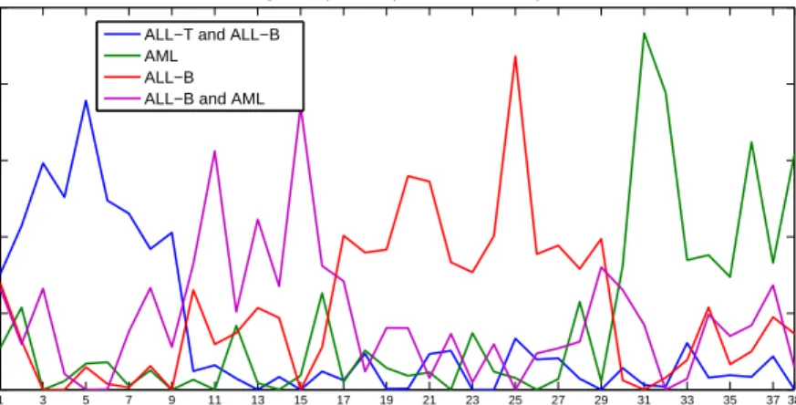
Figure 2.2: Metagenes expression patterns versus the samples for k = 4 in the
Leukemia dataset.
the sparse-NMF classification method presented in [64]. We first describe the gene expression dataset used and present the clustering procedure.
2.5.1 Data sets description. One of the important challenges in DNA mi-croarrays analysis is to group genes and experiments/samples according to their simi-larity in gene expression patterns. Microarrays simultaneously measure the expression levels of thousands of genes in a genome. The microarray data can be represented by
a gene-expression matrix V ∈ Rn×m , where n is the number of genes and m is the
number of samples that may represent distinct tissues, experiments, or time points.
The mth column of V represents the expression levels of all the genes in the mth
sample.
We consider seven different microarray data sets: leukemia [10], medulloblas-toma [10], prostate [51], colon [2], breast-colon [13], lung [7] and brain [44]. The leukemia data set is considered a benchmark in cancer clustering and
classifica-Samples Samples K=2 5 10 15 20 25 30 5 10 15 20 25 30 5 10 15 20 25 30 5 10 15 20 25 30 5 10 15 20 25 30 5 10 15 20 25 30 K=3 5 10 15 20 25 30 5 10 15 20 25 30 5 10 15 20 25 30 5 10 15 20 25 30 5 10 15 20 25 30 5 10 15 20 25 30 K=4 5 10 15 20 25 30 5 10 15 20 25 30 5 10 15 20 25 30 5 10 15 20 25 30 5 10 15 20 25 30 5 10 15 20 25 30 K=5 5 10 15 20 25 30 5 10 15 20 25 30 5 10 15 20 25 30 5 10 15 20 25 30 5 10 15 20 25 30 5 10 15 20 25 30 0 0.2 0.4 0.6 0.8 1 (a) (b)
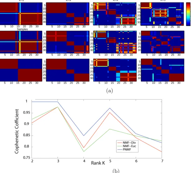
Figure 2.3: Clustering results for the Medulloblastoma dataset: (a) Consensus matri-ces: Top row NMF-Euc, Second row NMF-Div, bottom row: PNMF; (b) Cophenetic
coefficient versus the rank k (NMF-Euc in green, NMF-Div in red and PNMF in
tion [10]. The distinction between acute myelogenous leukemia (AML) and acute lymphoblastic leukemia (ALL), as well as the division of ALL into T and B cell sub-types, is well known [10]. We consider an ALL-AML dataset, which contains 5000 genes and 38 bone marrow samples (tissues from different patients for the considered genes) [10]. The considered leukemia dataset contains 19 ALL-B, 8 ALL-T and 11 AML samples.
The medulloblastoma data set is a collection of 34 childhood brain tumors samples from different patients. Each patient is represented by 5893 genes. The pathogen-esis of these brain tumors is not well understood. However, two known histological subclasses can be easily differentiated under the microscope, namely, classic (C) and desmoplastic (D) medulloblastoma tumors [10]. The medulloblastoma dataset con-tains 25 C and 9 D childhood brain tumors.
The prostate data [51] contains the gene expression patterns from 52 prostate tumors (PR) and 50 normal prostate specimens (N), which could be used to pre-dict common clinical and pathological phenotypes relevant to the treatment of men diagnosed with this disease. The prostate dataset contains 102 samples across 339 genes.
The colondataset [2] is obtained from 40 tumors and 22 normal colon tissue sam-ples across 2000 genes. The breast and colon data [13] contains tissues from 62 lymph node-negative breast tumors (B) and 42 Dukes’ B colon tumors (C). The lung tumor data [7] contains 17 normal lung tissues (NL), 139 adenocarcinoma (AD), 6 small-cell lung cancer (SCLC), 20 pulmonary carcinoids (COID) and 21 squamous cell lung carcinomas (SQ) samples across 12600 genes. The brain data [44] is the collection of
embryonal tumors of the central nervous system. This data includes 10 medulloblas-tomas (MD), 10 malignant gliomas (Mglio), 10 atypical teratoid/rhabdoid tumors (Rhab), 4 normal tissues (Ncer) and 8 primitive neuroectodermal tumors (PNET). The brain samples are measured across 1379 genes.
2.5.2 Gene expression data clustering. Applying the NMF framework to
data obtained from gene expression profiles allows the grouping of genes asmetagenes
that capture latent structures in the observed data and provide significant insight into underlying biological processes and the mechanisms of disease. Typically, there are a few metagenes in the observed data that may monitor several thousands of genes. Thus, the redundancy in this application is very high, which is very profitable for
NMF [14]. Assuming gene profiles can be grouped intojmetagenes,V can be factored
with NMF into the product of two non-negative matrices W ∈Rn×j and H ∈
Rj×m.
Each column vector of W represents a metagene. In particular, wij denotes the
contribution of theith genes into the jth metagene, and h
jm is the expression level of
the jth metagene in the mth sample.
Clustering performance evaluation
The position of the maximum value in each column vector of H indicates the index
of the cluster to which the sample is assigned. Thus, there are j clusters of the
to the same cluster, and cij = 0 otherwise. The connectivity matrix from each run of NMF is reordered to form a block diagonal matrix. After performing several runs, a
consensus matrix is calculated by averaging all the connectivity matrices. The entries of the consensus matrix range between 0 and 1, and they can be interpreted as the
probability that samplesiandj belong to the same cluster. Moreover, if the entries of
the consensus matrix were arranged so that samples belonging to the same cluster are adjacent to each other, perfect consensus matrix would translate into a block-diagonal matrix with non-overlapping blocks of 1’s along the diagonal, each block correspond-ing to a different cluster [10]. Thus, uscorrespond-ing the consensus matrix, we could cluster the
samples and also assess the performance of the number of clusters k. A quantitative
measure to evaluate the stability of the clustering associated with a cluster number
k was proposed in [31]. The measure is based on the correlation coefficient of the
consensus matrix, ρk, also called the cophenetic correlation coefficient. This
coef-ficient measures how faithfully the consensus matrix represents the similarities and
dissimilarities among observations. Analytically, we haveρk = m12
P
ij4(cij−
1 2)
2 [31].
Observe that 0≤ρk ≤1, and a perfect consensus matrix (all entries equal to 0 or 1)
would have ρk = 1. The optimal value of k is obtained when the magnitude of the
cophenetic correlation coefficient starts declining.
Clustering results
Brunet et al. [10] showed that the (deterministic) NMF based on the divergence cost
divergence cost function is defined as (W∗, H∗) = arg min W,H≥0 g(W, H) =X i,j (Vijlog( Vij (W H)ij ) − Vij + (W H)ij) (2.19)
The update rules for the divergence function are given by [33]
Hij ←− Hij P k(WkiVkj)/(W H)kj P rWri Wij ←− Wij P k(HjkVik)/(W H)ik P rHjr (2.20)
In this section, we compare the PNMF algorithm in (2.12) with both the Euclidean-based NMF in (2.5) and the divergence-Euclidean-based NMF in (2.19). We propose to cluster the leukemia and the medulloblastoma sample sets because the biological subclasses of these two datasets are known, and hence we can compare the performance of the algorithms with the ground truth. Figure 2.1(a) shows the consensus matrices
corre-sponding to k = 2,3,4 clusters for the leukemia dataset. In this figure, the matrices
are mapped using the gradient color so that dark blue corresponds to 0 and red to 1. We can observe the consensus matrix property that the samples’ classes are laid in block-diagonal along the matrix. It is clear from this figure that the PNMF performs better than the NMF algorithm, in terms of samples’ clustering. Specifically, the clusters, as identified by the PNMF algorithm, are better defined and the consensus
accuracy than the deterministic NMFs (based on the Euclidean and divergence costs).
Consistent clusters are also observed for rank k = 3, which reveal further portioning
of the samples when the ALL samples are classified as the B or T subclasses. In
particular, the nested structure of the blocks for k = 3 corresponds to the known
subdivision of the ALL samples into the T and B classes. Nested and partially over-lapped clusters can be interpreted with the NMF approaches. Nested clusters reflect local properties of expression patterns, and overlapping is due to global properties of multiple biological processes (selected genes can participate in many processes) [14].
An increase in the number of clusters beyond 3 (k = 4) results in stronger dispersion
in the consensus matrix. However, Fig. 2.1(b) shows that the value of the PNMF cophenetic correlation for rank 4 is equal to 1, whereas it drops sharply for both the Euclidean and divergence-based NMF algorithms. The Hierarchal Clustering (HC) method is also able to identify four clusters [10]. These clusters can be interpreted as subdividing the samples into sub-clusters that form separate patterns within the
whole set of samples as follows: {(11 ALL-B), (7 ALL-B and 1 AML), (8 ALL-T and
1 ALL-B), (10 AML)}.
Figure 2.2 depicts the metagenes expression profiles (rows ofH) versus the samples
for the PNMF algorithm. We can visually recognize the different four patterns that PNMF and HC are able to identify.
Figure 2.3 shows the consensus matrices and the cophenetic coefficients of the
medulloblastoma dataset for k = 2,3,4,5. The NMF and PNMF algorithms are able
to identify the two known histological subclasses: classic and desmoplastic. They also
5000 750 1000 1250 1500 1750 2000 2250 2500 2750 3000 3250 3500 3750 4000 4250 4500 4750 5000 2.5 5 7.5 10 12.5 15 17.5 20 22.5 25 27.5 30 32.5 35 Number of Genes Percentage error
Clustering Error (%) vs Number of Genes in Leukemia Data for K=2
NMF−Div NMF−Euc PNMF K−means HC (maxclust)
Figure 2.4: (NMF-Euc in green, NMF-Div in red and PNMF in blue, K-means in
black and Hierarchical Clustering in purple ) in Leukemia dataset fork = 2.
of the high values of the cophenetic coefficient for k = 3,5 and the steep drop off for
k = 4,6. The sample assignments for k = 2,3 and 5 display a nesting of putative
medulloblastoma classes, similar to that seen in the leukemia dataset. From Fig. 2.3, we can see that the PNMF clustering is more robust, with respect to the consensus matrix and the cophenetic coefficient, than the NMF clustering. Furthermore, Brunet
et al. [10] stated that the divergence-based NMF is able to recognize subtypes that the Euclidian version cannot identify. We also reach a similar conclusion as shown in
Fig. 2.3 for k = 3,5, where the Euclidian-based NMF factorization shows scattering
from these structures. However, the PNMF clustering performs even better than the divergence-based NMF as shown in Figs. 2.3(a) and 2.3(b).
To confirm our results we compare our proposed PNMF algorithm with the stan-dard NMF algorithms, distance criterion-based Hierarchical Clustering (HC) and K-means. We plot in figure 2.4 the curve Error vs. Number of genes in the labeled Leukemia data set. We select genes with small profile variance using the
Bioinfor-0,01 0,1 0,2 0,3 0,4 0,5 0,6 0,7 0,8 0,9 1 1,1 1,2 1,3 1,4 1,5 0.8 0.82 0.84 0.86 0.88 0.9 0.92 0.94 0.96 0.98 1 Standard deviation σ Cophenetic coefficient ρ
Copehenetic coefficient vs. Standard deviation of the measurement noise for K=2,3,4
K=2 K=3 K=4
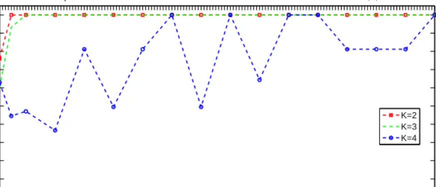
Figure 2.5: The cophenetic coefficient versus the standard deviation of the
measure-ment noise for k = 2 (red), 3 (green) and 4 (blue) in the Leukemia dataset.
are equally spaced. We run 100 Monte Carlo simulation then we take the average of the error. Our simulation results show that PNMF outperforms other clustering approaches.
Robustness evaluation
In this subsection, we assess the performance of the PNMF algorithm with respect to the model parameters, especially the choice of the noise power. Recall that, in the
probabilistic model, σ measures the uncertainty in the data or the noise power in the
gene expression measurements. We set the prior standard deviationsσW =σH = 0.01,
and compute the cophenetic coefficient for varying values ofσ between 0.01 and 1.5.
Figure 2.5 shows the cophenetic coefficient versus the standard deviation σ in the
leukemia data set for ranks k = 2,3,4. We observe that the PNMF is stable to
a choice of σ between 0.05 and 1.5 for the ranks k = 2 and 3, which correspond to
biologically relevant classes. In particular, whenσtends to zero, the PNMF algorithm
−109.5 −99.5 −89.5 −79.5 −69.5 −59.5 −49.5 −39.5 −29.5 −19.50 −9.5 0.5 10.5 20.5 30.5 40.5 50.5 60.5 70.5 80.5 90.5100.5 110.5 120.5 130.5 0.1 0.2 0.3 0.4 0.5 0.6 0.7 0.8 0.9 1 1.1 1.1 For K=2 SNR/dB Cophenetic coefficient Det−Div Det−Euc PNMF −109.5 −99.5 −89.5 −79.5 −69.5 −59.5 −49.5 −39.5 −29.5 −19.50 −9.5 0.5 10.5 20.5 30.5 40.5 50.5 60.5 70.5 80.5 90.5100.5 110.5 120.5 130.5 0.1 0.2 0.3 0.4 0.5 0.6 0.7 0.8 0.9 1 1.1 1.1 SNR/dB Cophenetic coefficient For K=3 Det−Div Det−Euc PNMF
Figure 2.6: Cophenetic versus SNR in dB (NMF-Euc in green, NMF-Div in red and
PNMF in blue) in Leukemia dataset for k = 2 andk = 3.
values of σ near zero.
We next study the robustness of the NMF and the proposed PNMF algorithms to the presence of noise in the data. To this end, we add white Gaussian noise, with varying power, to the leukemia dataset according to the following formula,
Vnoisy =V +σnR, (2.21)
−109.68−99.68 −89.68 −79.68 −69.68 −59.68 −49.68 −39.68 −29.68 −19.68 −9.680 0.31 10.31 20.31 30.31 40.31 50.31 60.31 70.31 80.31 90.31 100.31 110.31 120.31 130.31 0.2 0.4 0.6 0.8 1 SNR/dB Cophenetic coefficient For K=2 Det−Div Det−Euc PNMF −109.68−99.68 −89.68 −79.68 −69.68 −59.68 −49.68 −39.68 −29.68 −19.68 −9.680 0.31 10.31 20.31 30.31 40.31 50.31 60.31 70.31 80.31 90.31 100.31 110.31 120.31 130.31 0.2 0.4 0.6 0.8 1 SNR/dB Cophenetic coefficient For K=3 Det−Div Det−Euc Stoch
Figure 2.7: Cophenetic versus SNR in dB (NMF-Euc in green, NMF-Div in red and
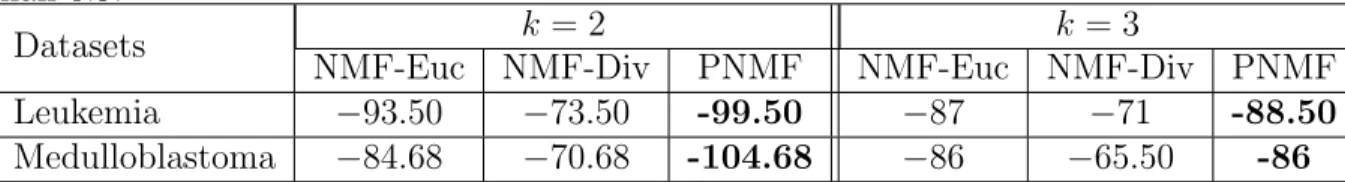
Table 2.1: Smallest SNR value for which the cophenetic coefficient is higher or equal
than 0.9.
Datasets k= 2 k= 3
NMF-Euc NMF-Div PNMF NMF-Euc NMF-Div PNMF
Leukemia −93.50 −73.50 -99.50 −87 −71 -88.50
Medulloblastoma −84.68 −70.68 -104.68 −86 −65.50 -86
by SNR = PV
σ2
n, where the signal power PV =
1 nm P i P jv 2 ij = nm1 kVk 2 F. Since the
cophenetic coefficient measures the stability of the clustering, we plot in Figures
2.6 and 2.7 the cophenetic coefficient versus the SN R, measured in dB, for both
the Euclidean-based and divergence-based NMFs and PNMF algorithms using the leukemia and medulloblastoma data sets. We observe that the PNMF algorithm leads
to more robust clustering than the deterministic NMF algorithms for allSN Rvalues.
Table 2.1 shows the minimum SNR values for which the cophenetic coefficient takes values higher or equal than 0.9. We say that the algorithm is ”stable” for SNR values higher or equal than the minimum SNR. For the leukemia data, the Euclidean-based
NMF and the divergence-based NMF algorithms stabilize respectively at SN R =
−93.5 and SN R = −73.5 dB for k = 2, whereas the PNMF algorithm is stable at
lower SNR values, SN R = −99.5 dB for k = 2. Similar results are obtained for
the medulloblastoma dataset, where the NMF algorithms stabilize respectively as
above at SN R = −84.68 and SN R = −70.68 dB, whereas the PNMF is stable at
SN R=−104.68 dB. Thus, the PNMF algorithm is more stable than its deterministic
homologue. Also, observe that the Euclidian-based NMF performs better than its divergence homologue for noisy data.
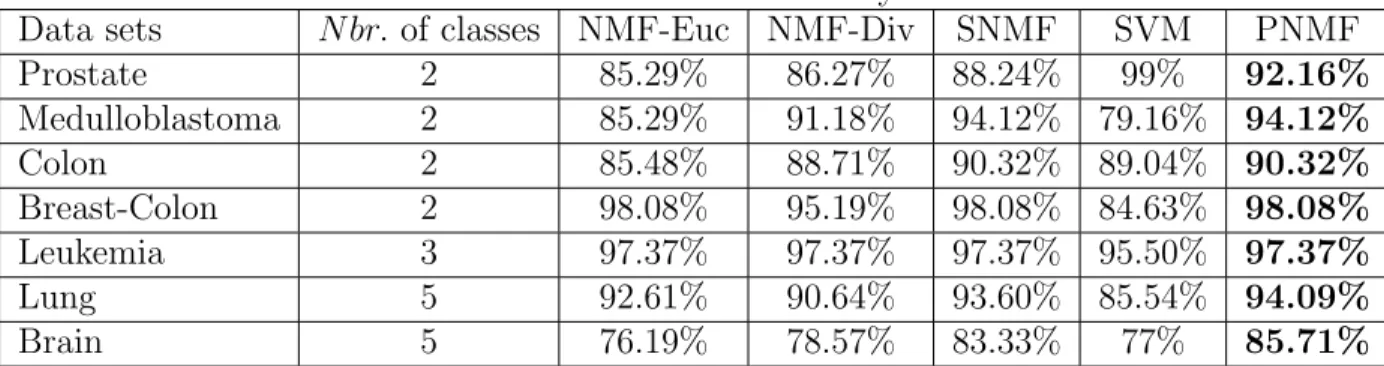
2.5.3 NMF-based tumor classification. Given that the proposed PNMF algorithm results in more stable clustering than its deterministic homologue, we ex-pect that it will also lead to better feature extraction and classification. We classify the tumors in the seven gene expression datasets described in Section 2.5.1.
We assess the performance of the classification algorithm using the 10-fold
cross-validation technique [64]. The number of metagenes ki can be determined using the
nested stratified 10-fold cross-validation. However, we follow the work in [64] and
choose ki = 8 if the number of samples in the ith class ri >8. Otherwise we choose
ki =ri. We selected the parametersαandβof PNMF in order to minimize the
classifi-cation error in the training dataset based on a 10-fold cross-validation technique. The parameters of SNMF were selected using the same criterion and method, i.e. minimize the classification error in the training dataset. The classification results for the NMF, PNMF, SVM and SNMF [64] algorithms are summarized in Table 2.2. In particular, we compared the PNMF-based MSRC algorithm to the SVM algorithm which has been shown to outperform K-NN and neural network in tumor classification [52], [43]. In our experiment we use one-versus-rest SVM (OVRSVM) with Polynomial kernels approach which has been shown to be the best one [52]. The results can be ob-tained using the Gene Expression Model Selector (GEMS) publicly available online
http://www.gems-system.org/. Observe that the PNMF-based classifier performs
better than the other approaches for the considered data sets except for the prostate data where SVM achieves the highest classification accuracy. Moreover, the PNMF performs better than the SNMF for the prostate, lung and brain data sets. This
Table 2.2: Classification accuracy
Data sets N br. of classes NMF-Euc NMF-Div SNMF SVM PNMF
Prostate 2 85.29% 86.27% 88.24% 99% 92.16% Medulloblastoma 2 85.29% 91.18% 94.12% 79.16% 94.12% Colon 2 85.48% 88.71% 90.32% 89.04% 90.32% Breast-Colon 2 98.08% 95.19% 98.08% 84.63% 98.08% Leukemia 3 97.37% 97.37% 97.37% 95.50% 97.37% Lung 5 92.61% 90.64% 93.60% 85.54% 94.09% Brain 5 76.19% 78.57% 83.33% 77% 85.71%
is due to the high accuracy of the PNMF in feature extraction as compared to the SNMF algorithm, which is not guaranteed to converge to the optimal non-negative factorization [64].
2.6 Conclusion and Discussion
Studying and analyzing tumor profiles is a very relevant area in computational bi-ology. Clinical applications include clustering and classification of gene expression profiles. In this work, we developed a new mathematical framework for clustering and classification based on the Probabilistic Non-negative Matrix Factorization (PNMF) method. We presented an extension of the deterministic NMF algorithm to the proba-bilistic case. The proposed PNMF algorithm takes into account the stochastic nature of the data due to the inherent presence of noise in the measurements as well as the internal biological variability. We subsequently casted the optimal non-negative probabilistic factorization as a weighted regularized matrix factorization problem.
rules for the NMF algorithm. We have also generalized Lee and Seung’s algorithm to include a general class of update rules, which converge towards a stationary point of the (deterministic) NMF problem. We next derived a PNMF-based classifier, which relies on the PNMF factorization to extract features and classify the samples in the data. The PNMF-based clustering and classification algorithms were applied to seven microarray gene expression datasets. In particular, the PNMF-based clustering was able to identify biologically significant classes and subclasses of tumor samples in the leukemia and medulloblastoma datasets. Moreover, the PNMF clustering results were more stable and robust to data corrupted by noise than the classic (deterministic) NMF.
Thanks to its high stability, robustness to noise and convergence properties, the PNMF algorithm yielded better tumor classification results than the NMF and the Sparse NMF (SNMF) algorithms. The proposed PNMF framework and algorithm can be further applied to many other relevant applications in biomedical data pro-cessing and analysis, including muscle identification in the nervous system, image classification, and protein fold recognition.
Chapter 3
SMURC: High-Dimension Small-Sample Multivariate Regression with Covariance Estimation
3.1 Introduction
Many engineering problems are formulated as an inverse problem. Examples in signal processing include source estimation of electroencephalographic (EEG) and magne-toencephalographic (MEG) data and inference or reverse-engineering of genetic reg-ulatory networks from high-throughput gene expression data. These problems are
sometimes referred to as ill-posed or ill-defined because the inverse problem has no
unique solution, and there are infinitely many solutions that are equally compati-ble with the data. For instance, in EEG and MEG source estimation procompati-blems, if the source distribution contains more independent parameters than there is indepen-dent information in the recorded data, then the sources spatial distribution cannot be estimated. In genomics, the inference of genetic regulatory networks also suffers from the limited number of measurements available to unambiguously estimate the
network connectivity. This problem, known as the “large p small n” problem, poses
The approaches proposed in the literature to tackle inverse problems can be clas-sified into three groups: (1) the statistical approach, which finds the most likely solution that fits the data and any additional constraints that may be imposed; (2) the minimum norm approach, which finds a solution that is compatible with the data and satisfies additional constraints, e.g., on the amplitudes or covariances of the pa-rameters; (3) the resolution optimization methods, which estimate the parameters as independently as possible from each other. It has been shown in [26] that all these approaches result in the same solution given the same a priori information. Moreover, if no a priori information is available, all three methods are equivalent to the classical minimum norm solution [26].
Let us consider the (under-determined) multivariate regression problem, which
generalizes the classical regression problem of one response on p predictors to
re-gressing q responses on p predictors. This model has various applications including
genomics [42], neurology [35], imaging [35] and econometrics. Let xi = (xi1,· · · , xip)
denote the predictors, yi = (yi1,· · · , yiq) denote the responses, and i = (i1,· · · , iq)
the errors for the ith sample. The multivariate regression model is given by
yi =Axi+i, i= 1,· · · , n, (3.1)
whereAis aq×p regression matrix andn is the sample size. We make the standard
Σ, i.e.,i ∼ N(0,Σ). The model in (3.1) can be expressed in matrix notation as
Y =AX+E, (3.2)
whereY is the q×n response matrix with itsith columny
i,X is the p×n predictor
matrix with its ith column x
i and E is the random error matrix. X is assumed to
be full-rank. The system is under-determined when there are more parameters than samples, i,e, q > p > n.
The negative log-likelihood function of (A,Ω),Ω=Σ−1, can be expressed up to
a constant as, g(A,Ω) = tr 1 n(Y −AX) tΩ(Y −AX) −log|Ω|, (3.3)
where tr denotes the trace operator. If p≤n (complete or over-determined system),
the maximum likelihood estimator forAis simply given by ˆAOLS=Y XT(XXT)−1,
which is independent of Ω and amounts to performing q separate ordinary
least-squares.
The multivariate regression problem becomes particularly challenging when the
system is under-determined as it requires the estimation of pq parameters fromnq <
qp predictors or n < p. Different approaches were proposed to reduce the number of
parameters by minimizing (3.3) under various constraints on the regression matrix
a sparsity constraint on the singular values ofA[61]. Sparsity can also be imposed to
identify the main predictors [42], where a combined constraint function that includes
l1andl2regularization, is used [40]. Thel1constraint introduces sparsity in the entries
of A and the l2 regularization identifies irrelevant predictors (for all q responses) by
introducing zeros for all entries in some rows of A. However, all of these approaches
do not account for correlated responses.
Exploiting the correlation in the response variables improves the prediction per-formance. For under-determined problems, however, the maximum likelihood (ML) approach with covariance estimation is senseless because there exist solutions
satisfy-ing Y =AX and Σinfinitely small. For these solutions, the negative log-likelihood
in (3.3) tends to−∞. Hence, the likelihood, as a function of the two variables (A,Ω),
diverges. Observe that the likelihood converges if the covariance matrix Σis known
(e.g., proportional to the Identity for uncorrelated measurements) or if the system is
over-determined (in this case, there exists no solution that satisfies Y =AX).
Rothman et al. [48] proposed a regularized algorithm that simultaneously infers
the regression coefficient matrix A and the inverse error covariance, Ω = Σ−1, by
imposing sparsity constraints on Ω. The l1-norm penalty on Ω ensures the
conver-gence of the regularized likelihood because it excludes exact solutions, for which the covariance is infinitely small or equivalently the inverse covariance is infinitely large. However, in many applications, the assumption of a sparse inverse covariance matrix may not be reasonable or have any physical justification. In particular, in the genetic regulatory network problem, there is no evidence for such an assumption. Moreover, the solution to the regularized problem in [48] relies on an iterative procedure that
finds the maximum over A then over Ω. That is because the problem is convex in
each variable, A and Ω, but not convex in the pair (A,Ω). This iterative procedure
is not guaranteed to converge and if it does converge, then it may not reach the opti-mal solution. Additionally, the authors observed that this algorithm may take many iterations to converge for high-dimensional data. Subsequently, they proposed an ap-proximate MRCE approach that prematurely terminates the iterative optimization procedure after two iterations.
Recently, Zhang et al. [62] proposed the sparse Conditional Gaussian Graphical
Model (sCGGM). CGGM formulates the inference problem as a joint probabilistic
graphical model. sCGGM minimizes the negative log-likelihood of the data with l1
penalties on the autocorrelation and cross-correlation precision matrices [62]. The main advantage of CGGM over MRCE is that CGGM leads to a convex problem, whereas the MRCE estimation problem is only bi-convex, not jointly convex. How-ever, as acknowledged by the authors, CGGM and MRCE are so similar that “MRCE was mistakenly called a sparse CGGM” [62]. In essence, both algorithms solve an under-determined linear regression problem by maximizing the Gaussian likelihood subject to sparse constraints on the correlation structure. Hence, the open question remains: “How can we perform maximum likelihood with covariance estimation for under-determined systems?”
The work that we present in this chapter addresses this question, namely the problem of ML estimation with unknown covariance in under-determined systems.
In this chapter, scalars are denoted by lower case letters, e.g., n, m; vectors are
denoted by bold lower case letters, e.g., x,y; and matrices are referred to by bold
upper case letters, e.g., A,X. I denotes the identity matrix. xi denotes the ith
element of vectorxand aij is the (i, j)th entry of matrixA. Throughout the chapter,
we provide references to known results and limit the presentation of proofs to new contributions.
3.2 The Normalized-Likelihood
We propose to weight the likelihood function by the “energy” of the error, in order to guarantee the convergence of the energy-weighted likelihood function, while still keeping the exponential form of the density. Specifically, we define the
normalized-likelihood of the under-determined (p > n) multiple regression model in (3.2), under
the Gaussian assumption, as
Definition 3.2.1. LN(A,Ω) = | (Y −AX)TΩ(Y −AX)|n2 (2π)np2 exp[−1 2Tr[(Y −AX)TΩ(Y −AX)]], (3.4)
where | · | is the matrix determinant operator.
Obviously, one can propose many possible normalizations of the Gaussian
likeli-hood as a function of the pair (A,Ω). Our particular “choice” in Definition 3.2.1
while keeping the form of the Gaussian density. This normalization of the Gaussian
likelihood avoids exact solutions and subsequent divergence issues. The pair (A,Ω)
can then be computed to maximize the normalized-likelihood, LN, i.e.,
(A∗,Ω∗) = arg max
A,Ω
LN(A,Ω), (3.5)
Proposition 3. The solution to (3.5) is given by
(Y −A∗X)TΩ∗(Y −A∗X) =nI, (3.6)
where I denotes the n×n Identity matrix.
Proof of Proposition 3. Let Z = (Y −AX)TΩ(Y −AX). Then, the
normalized-likelihood can be written as the following function of the variable Z,
LN(Z) = |
Z|n2
(2π)nq2
exp−1
2Tr[Z]. (3.7)
To find the stationary point Z∗, we set ∂LN(Z)
∂Z =0. ∂LN(Z) ∂Z = n 2|Z| n 2−1|Z|Z−1exp−1 2Tr[Z] − 1 2|Z| n 2 exp−1 2Tr[Z] = 1 2|Z| n 2[nZ−1−I] exp−1 2Tr[Z] = 0
Moreover, it can be easily derived that the Hessian at the stationary pointZ∗is given by ∂2L N(Z) ∂Z2 |Z=Z ∗=− 1 2nn n2 2 e− n2 2 <0 (3.9)
There are many pairs (A∗,Ω∗), which satisfy equality (3.6) and hence maximize
the normalized-likelihood. The non-uniqueness of the solution is not surprising given that the problem is under-determined. Among all possible solutions of (3.6), we
propose to find those that minimize the regularized errorkY −AXk2
F+λkΩk2F, where
λ is a tuning parameter and k · kF denotes the Frobenius norm. Observe that it is
meaningful to consider the error as the objective function here, because the set of pairs
(A,Ω) satisfying (3.6) are not exact solutions, i.e., they do not satisfy the equality
Y =AX, and hence the minimum error is not trivially zero. Thus, an advantage of
the normalized-likelihood is that it avoids considering exact solutions. In addition,
we consider constraints on the regression matrix A, which reflect prior knowledge
about the nature of the regression model. For instance, A may be constrained to
be sparse. Many applications assume a sparse regression matrix, e.g., robust face recognition, where the target can be represented as a sparse linear combination of the dataset [58] and structural equation models (SEM) to infer gene or phenotype
constrained optimization problem, thus, becomes min (A,Ω)kY −AXk 2 F +λkΩk2F s.t. (Y −AX)TΩ(Y −AX) =nI, A∈ A. (3.10)
Problem (3.10) is formulated in terms of the two coupled variables Aand Ω, which
satisfy (3.6) to maximize the normalized-likelihood function. The following lemma
derives an analytical expression of Ω as a function of A, and hence reduces the
problem to depend on only one variable A. Before stating the lemma’s result, we
need the following definition of the polar decomposition of matrices.
Definition 3.2.2. The polar decomposition of a matrix B ∈Cp×n is given by
B =U|B|, (3.11)
where |B| = (BTB)1/2, (·)1/2 is the principal square root operator and U :
Cn −→
Range(B) is a Cp×n isometry such that UTU =I.
Lemma 3.2.3. GivenA, there exist manyΩsatisfying equality (3.6). The minimum Frobenius norm Ω, for a fixed A, is given by
ΩA=n U
(Y −AX)T(Y −AX)−1
Proof of Lemma 3.2.3. Let B = (Y −AX). Consider the polar decomposition of
B given by
B =U|B|, and |B|= (BTB)1/2. (3.13)
Then, the equality in (3.6) becomes
(Y −AX)TΩ(Y −AX) =nI
⇐⇒ BTΩB =nI
⇐⇒ |B|UTΩU|B|=nI
⇐⇒ UTΩU =n|B|−2 (3.14)
Since UTU = I, UT restricted to the range of B is invertible, i.e., UT Range(B) is
invertible. Let us write
Cq= Range(B)⊕Ker(BT), (3.15)
where ⊕ denotes the direct sum of the two subspaces Range(B) and Ker(BT). Let
PB be the orthogonal projection onto Range(B). Then, we can decomposeΩ as
Ω=PBΩPB⊕PBΩPB⊥⊕PB⊥ΩPB⊕PB⊥ΩPB⊥, (3.16)
where P⊥B is the orthogonal projection onto the orthogonal space of Range(B), i.e.,
properties:
PB⊥U =UTPB⊥ =0. (3.17)
Thus, from the decomposition of the matrix Ω in Eq. (3.16), we obtain
UTΩU = UTPB ΩPBU. (3.18)
From Eq. (3.14) and since UT Range(B) is invertible, we have
UTΩU =UTPB ΩPBU =n|B|−2
⇐⇒
PB ΩPB =n U|B|−2UT. (3.19)
From the matrix decomposition in (3.16), for a fixed A, PB Ω PB is fixed. Thus,
the minimum Frobenius norm matrix Ω results by setting the three other terms in
the matrix decomposition to zero, i.e., the minimum Frobenius norm matrix is of the form
Ω=PB Ω PB. (3.20)
The result of Lemma 3.2.3 then follows from Eqs. (3.19) and (3.20).
prob-Proposition 4. The optimization problem in (3.10) is equivalent to min S Tr(S 2 ) +λ n2Tr(S−4) s.t. S =|Y −AX|, A∈ A (3.21)
Proof of Proposition 4. Replacing ΩA in the objective function of the optimization
problem (3.10) by its expression obtained in Lemma 3.2.3, and lettingB =Y −AX,
we obtain kY −AXk2F +λkΩk2F = kBkF2 +λkn2U(BTB)−1UTk2F = Tr(BTB) +λn2 Tr(U(BTB)−1UTU(BTB)−1UT) = Tr(BTB) +λn2Tr((BTB)−2) = Tr(S2) +λn2Tr(S−4), (3.22) where S2 =BTB = (Y −AX)T(Y −AX).
Though the objective function in (3.21) is convex (as a function of the variable
S), the equality in the constraint (assuming that A is convex) is not affine and
thus the optimization problem (3.21) is not convex [9]. We will, therefore, relax the minimization of (3.21) to a minimization over a convex set that is included in the
original set. In what follows, we show that if the matrix regression A is sparse with
a convex optimization problem. Moreover, this approximation formulates a much simpler optimization problem than the initial setting in (3.21) because it depends
only on S and is independent of A.
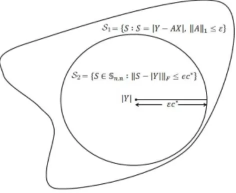
Proposition 5. If A={A:kAk1 ≤}, then the optimization problem in (3.21) can
be approximated by the following convex optimization problem
min S Tr(S 2) +λ n2Tr(S−4) s.t. S ∈Λ ={S ∈Sn,n : kS− |Y|kF ≤c∗} (3.23)
where Sn,n is the set of n×n symmetric positive semi-definite matrices and c∗ is a
small term which depends on X, Y but independent of .
Proof of Proposition 5. Let
S1 ={S :S =|Y −AX|,kAk1 ≤}. (3.24)
and let
S2 ={S ∈Sn,n:kS − |Y|kF ≤c∗}. (3.25)
We will show that S2 ⊆ S1. An illustration of these two sets is provided in Fig. 3.1.
To this aim, we considerS ∈ S2 and show that S ∈ S1. Specifically, givenS ∈ S2 we
Figure 3.1: Approximation of the optimization problem in Proposition 4 by the convex
optimization problem in Proposition 5. Illustration of the setsS1 andS2 in the proof
of Proposition 5.
matrix A satisfying the previous identity. We will construct a specific matrix A.
Namely, we fix U = V, where V is the isometry from the polar decomposition
Y =V|Y|. Then, we need to findA such that
AX =V(|Y| −S). (3.26)
X is full-rank; hence invertible from the right. Let us define
˜ X = X−1 Range(X), 0 [Range(X)]⊥ (3.27)
From the Definition of ˜X, we haveAXX˜
Range(X) =A Range(X)andAXX˜ Range(X)⊥ =
0. Therefore, multiplying Eq. (3.26) to the right by ˜X, we see that A defined by
A= V(|Y| −S) ˜X Range(X), 0[Range(X)]⊥ (3.28)