Off-Balance Sheet Financing and Bank Capital Regulation: Lessons
from Asset-Backed Commercial Paper
Jiakai Chen∗ Job Market Paper
February 6, 2015
Abstract
Many shadow banks rely heavily on bank-sponsored private credit and liquidity support, not government guarantees. The financial crisis demonstrated that bank capital regulation cannot be effective without explicitly considering these facilities. Using a continuous time model with maturity mismatch and bank moral hazard, I study the impact of credit and liquidity guarantees on bank capital structure. I focus on a particular type of shadow banking called asset-backed commercial paper (ABCP). When banks provide credit guarantees to ABCP conduits, assuming that the validity of the guarantees is ensured by rating agencies, the commercial paper becomes risk free and is always priced at par. Rolling over the commercial paper is thus costless, so that frequently rolling over the short term ABCP to fund long term assets—a maturity mismatch— has no impact on bank value. Regulators can eliminate a bank’s moral hazard by imposing a simple capital ratio requirement. However, the capital ratio requirement is no longer valid if banks use liquidity guarantees in their ABCP conduit funding because the funding maturity becomes important. Moreover, a liquidity guarantee becomes as costly as a credit guarantee when the maturity shortens. Using Moody’s ABCP conduit data, I confirm that shorter ABCP maturity causes the bank’s return to be more sensitive to the conduit credit loss. Thus, when banks have significant exposure to a liquidity guarantee, the search for a single appropriate risk weight is futile. More sophisticated tests, such as model-based tests are not only necessary but also have to be carried out under stressed scenarios.
Keywords: Capital regulation; Moral hazard; Rollover risk; Financial crisis; Maturity mismatch
JEL classification: D82, G01, G19, G23, G28, L51
∗
Haas School of Business, UC Berkeley. E-mail: jiakai chen@haas.berkeley.edu. I would like to thank Adam Ashcraft, Nicolae Garleanu, Amir Kermani, Hayne Leland, Christopher Palmer, David Skeie, Alexei Tchistyi, as well as the participants in the 2014 Joint Berkeley–Stanford Finance Student Seminar for helpful comments. I especially wish to thank Christine Parlour, Nancy Wallace, and Dwight Jaffee for their invaluable advice. Special thanks to Moody’s Investor Service, who provides the Asset-Backed Commercial Paper data. This research is supported by a research grant from Fisher Center for Real Estate and Urban Economics. For the latest version, please email me or visithttp://faculty.haas.berkeley.edu/jiakai_chen.
1
Introduction
Shadow banks carry out traditional banking activities—financing long-term illiquid assets with short-term liquid debt—outside the regulated banking sector. With less restrictive regulatory control, shadow banks usually have little access to traditional government sponsorship such as the central bank discount window or deposit insurance. Instead, shadow banks rely more on bank-sponsored private credit and liquidity facilities, which are often both complex and opaque. The recent financial crisis proved that the collapse of shadow banking can lead to large-scale bank failure. Thus, the regulation of these private credit and liquidity facilities has become an important, challenging, and controversial topic in the debate on post-crisis regulatory reform. In this paper, I analyze bank-sponsored credit and liquidity facilities in the asset-backed commercial paper (ABCP) program. I show that credit and liquidity facilities have different interactions with the maturity transformation, which can lead to ineffective regulation.
Asset-backed commercial paper or ABCP was an important part of the U.S. shadow-banking system. The ABCP market appeared in the mid-1980s and then grew rapidly, peaking in 2007 when it reached 1.21 trillion USD, about 12.3% the size of total U.S. commercial bank liability.1 Many researchers believe the growth of ABCP was mainly driven by regulatory arbitrage (see Adrian and Ashcraft (2012), Acharya et al. (2012), Pozsar et al. (2010), Gorton et al. (2010), and Ordonez (2013)). Specifically, regulators imposed capital requirements to curb the moral hazard encouraged by deposit insurance (see Decamps et al. (2004)). Such capital requirements increased banks’ funding costs, so banks turned to cheaper off-balance sheet funding channels, such as ABCP conduits. Briefly, a bank sponsoring such a conduit transfers assets to a separate trust, which funds the acquisition by issuing short-term commercial paper backed by the assets. Moving assets off-balance sheet reduces banks’ capital charge. To obtain cheap funding for the move, the sponsoring bank usually promises credit or liquidity guarantees to the commercial paper investors. On paper, the credit guarantee transmits the conduit’s credit risk to the bank, while under a liquidity guarantee the ABCP investors retain the credit risk.2
1
Source: Federal Reserve Bank St. Louis
2Section 2 contains an introduction to the institutional details of the ABCP program, credit guarantees, and liquidity guarantees.
Liquidity guaranteed ABCP conduits experienced three different regimes of accounting stan-dards and capital regulations in the 2000s. The first regime started in 2001, when Financial Accounting Standards (FAS) 140 was the prevailing accounting rule. FAS 140 effectively allowed banks to treat the asset transfer to a conduit as a true sale. Hence, there was no risk-capital requirement for using ABCP funding. However, after the Enron scandal, the Federal Accounting Standard Board (FASB) proposed a consolidation of conduits to balance sheets. The proposition raised concerns about ABCP conduit financing, and slowed down the growth of the ABCP market. The second regime started in 2004, when FASB issued Interpretation 46 (FIN 46) that required conduit assets to be consolidated onto banks’ balance sheets. However, the financial regulators amended the risk-based capital standards by allowing ABCP conduits to enjoy an “ABCP exclu-sion”, so that the conduit assets could be excluded from banks’ risk-weighted assets base after consolidation.3 As a result the ABCP market expanded rapidly, then shrank drastically following concerns about the housing market slow-down. The third regime started in 2010, when FAS 166 and 167 required banks to prepare allowance for loan and lease losses, which is included in tier 2 risk capital. The financial regulators also dropped the ABCP exclusion.4 A benefit to banks
of using an ABCP conduit is the reduced capital charge it has to hold against risky assets. Yet the benefit to a bank depends on whether investors view the assets as guaranteed and are willing to finance them at low rates. Given the complex relationship between off-balance sheet financing, investor behavior and bank moral hazard, can regulation of on-balance sheet activities curb banks’ moral hazard? How do investors value bank guarantees versus government guarantees? How do the various types of bank guarantees and commitments interact with prudential regulation?
To answer these questions, I present a dynamic framework in which a bank chooses its optimal capital structure by using ABCP funding in addition to traditional deposits.5 The regulator,
who also provides deposit insurance, tries to eliminate the moral hazard by setting capital ratio
3
Risk-Based Capital Guidelines; Capital Adequacy Guidelines; Capital Maintenance: Consolidation of Asset-Backed Commercial Paper Programs and Other Issues, 69 Fed. Reg. 44,908 (July 28, 2004), (to be codified at 12 C.F.R. pt. 3; 12 C.F.R. pts. 208, 225; 12 C.F.R. pt. 325; 12 C.F.R. pt. 567). Effective since September 30, 2004.
4Risk-Based Capital Guidelines; Capital Adequacy Guidelines; Capital Maintenance: Consolidation of Asset-Backed Commercial Paper Programs and Other Issues, 75 Fed. Reg. 4,636 (Jan 28, 2010), (to be codified at 12 C.F.R. pt. 3; 12 C.F.R. pts. 208, 225; 12 C.F.R. pt. 325; 12 C.F.R. pt. 567). Effective since March 29, 2010.
5
The dynamic capital structure model literature includes Leland (1994b), Leland and Toft (1996), Leland (1994a), and Decamps et al. (2004). The fair value of deposit insurance is related to Merton (1977) and Merton (1978), which studies the pricing of insurance under dynamic settings.
requirements. I show that when banks rely on deposits or ABCP funding with credit guarantees, perfect insurance of credit loss not only protects the investors, but also eliminates the bank’s rollover risk. Without the rollover risk, banks’ riskiness does not change with deposit maturity. Since the regulator demands banks that provide credit guarantees to prepare risk capital for 100% of the outstanding ABCP, risk-based capital ratio requirements are effective regulatory measures to control the moral hazard of banks using credit guaranteed ABCP conduit financing.
However, when banks use ABCP funding and provide liquidity guarantees to the commercial paper investors, they face rollover risk when they need to reissue new paper to replace the maturing paper. Rollover risk goes up when the maturity of the commercial paper becomes shorter. As a result, it is impossible to set an ‘appropriate’ risk capital requirement ex ante, without taking maturity mismatch into consideration.6
Furthermore, when the maturity of ABCP becomes short, the value of liquidity guarantees converges to that of credit guarantees.7 By allowing banks that provide liquidity guarantees to prepare risk capital for a fixed 10% of the outstanding ABCP, the regulator ignores the effect of ABCP maturity to the risk transfer between banks’ balance sheets and ABCP conduits. This helps to explain why some large U.S. financial institutions that failed during the financial crisis had core capital ratios well in excess of the regulatory minimum of 8%.
As Brunnermeier (2008) and Krishnamurthy (2009) point out, the excessive use of short-term debt financing is a major factor behind the notable collapse of large U.S. banks such as Bear Stearns. My result complements this literature by showing that the shortening of debt maturity not only adds to the liquidity pressure on the bank, but also imposes direct credit loss that the regulations failed to capture in the mid-2000s. My paper also extends several recent studies on rollover risk. Martin et al. (2014) study the fragility of short-term secured funding markets by investigating whether a run can occur as a result of changing market expectations. Acharya et al. (2011) show that high rollover frequency can lead to a market freeze, therefore lowers the maximum amount
6
Regulators also carry out liquidity coverage tests, which check whether the bank has enough cash (or equivalent short-term assets with good liquidity) to cover the short-term payment obligations. My model suggests there is actual credit loss on rolling over short-term commercial paper, in addition to the cashflow liquidity pressure.
7
ABCP in the United States has maturity ranging from overnight to 270 days, while in Europe the maturity usually ranges from overnight to 180 days.
that can be borrowed using good collateral. He and Xiong (2012b) study how deteriorating market liquidity leads to an increase in credit risk, originating from the firm’s debt rollover. In contrast, my paper focuses on the banking sector and studies the impact of rollover risk on the effectiveness of capital ratio regulation.
Using a proprietary dataset from Moody’s Investor Service, I verify that the maturity on the off-balance sheet ABCP conduits significantly affects banks’ equity value. Specifically, I analyze the relationship between banks’ returns and the size of the liquidity guarantees they provide to ABCP conduits, and the change in the commercial paper’s maturity. Using an instrumental variable that corrects for the simultaneity between banks’ returns and the maturity of ABCP conduits, I find that the interaction between the change in ABCP conduit maturity and the change in the underlying conduit riskiness measure significantly impacts banks’ equity returns. When subprime 2/28 adjustable-rate mortgage delinquency rate goes up by one standard deviation, about 3.3 basis points, for a bank with average obligation of liquidity guarantee to ABCP conduit, about 3.6% of its book value, and the fraction of outstanding ABCP maturing overnight raise by one standard error, about 1.137%, the U.S. banks experience about 7.5 to 11.3 basis points negative abnormal return. Both the theoretical and empirical results suggest that the capital regulation before 2009 did not correctly capture the riskiness of ABCP conduit liquidity guarantor.
The rest of the article is organized as follows. Section 2 describes the institutional details of ABCP conduits. I set up a benchmark model that describes the ABCP conduit with credit guarantees, as well as a model for the ABCP conduit with liquidity guarantees in section 3. I analyze the rational expectation equilibrium in the benchmark model, and the bounded rational equilibrium motivated by the capital regulation practice for ABCP with liquidity guarantees. I then test the key theoretical implication in section 4, showing that the change in ABCP maturity has a clear effect on the risk transfer from the conduit to the bank. Section 5 concludes the paper, and all technical proofs are given in the Appendix.
2
Institutional Details of ABCP Conduits
An ABCP conduit is a special purpose entity (SPE), established to fund a portfolio of long-term financial assets with commercial paper. A sponsoring bank creates an ABCP conduit, then transfers assets, such as Mortgage Backed Securities (MBS), from its balance sheet to the conduit. When the long-term underlying assets of the conduit are paid off, the bank replaces them by moving new assets to the conduit. The conduit funds any such purchases by issuing ABCP collateralized by the underlying assets. The conduit has a default threshold: when the underlying assets deteriorate such that the default threshold is crossed, the sponsoring bank has to wind down the ABCP conduit and pay off the ABCP investors.
Typically, ABCP is structured as short-term, senior secured debt. This is done to attract investment from money market funds. Under SEC Rule 2a-7, a money market fund may only hold the highest rated debt (a Prime-1 rating), which matures in under 13 months and must maintain an overall portfolio weighted average maturity of 60 days or less. This source of investment is large: Aggregate assets in money market funds were up to 2.69 trillion USD by the end of year 2008.8 The large size of money market funds leads to lower transaction costs of ABCP in the secondary market than those of equity or longer-term debt.
2.1 Credit vs. Liquidity Guarantees
For ABCP to obtain the desired Prime-1 rating, banks typically provide explicit guarantees to the ABCP investor upon the conduit default. There are two types of guarantees that banks can offer: credit guarantees or liquidity guarantees. Credit guarantees completely mitigate the ABCP investors’ credit loss upon conduit default, by paying the ABCP investor the full principal amount. It is thus akin to private deposit insurance offered by the sponsoring bank.
A liquidity guarantee, unlike a credit guarantee, does not cover the loss inflicted by the already defaulted assets when the ABCP conduit winds-down. Although the conduits usually have some credit enhancement measures, such as a subordinate or overcollateralization tranche as the first
8Source: Federal Reserve Financial Accounts of the United States: Flow of Funds, Balance Sheets, and Integrated Macroeconomic Accounts. First Quarter 2014.
group to absorb the loss of the defaulted assets, the ABCP investors are still subject to credit risk once the credit enhancement is depleted.9 Specifically, if a conduit with a liquidity guarantee defaults, its ABCP investors will only recover the remaining collateral value of the underlying assets.
Rollover support The sponsoring bank also helps the rollover of commercial paper when the investors with maturing ABCP no longer want to reinvest. In this case, the sponsoring bank pays the commercial paper’s principal amount back to the ABCP investors, therefore making sure that the ABCP investor can always recover their principal when the conduit has not reached the default threshold. The bank then reissues ABCP, usually at a discounted price. The short maturity of ABCP allows the ABCP investors to liquidate their investment by not rolling over maturing paper if they believe the underlying assets are deteriorating.
Conduit wind down The use of off-balance sheet funding is critical to modern banks’ business model. If a sponsoring bank ever allows the ABCP investors to fire-sale the commercial paper upon the default of the conduit, it would lack the credibility to continue placing assets in any other conduits. Hence, it is in the bank’s interest to promise to consolidate a conduit back into its balance sheet when the conduit’s underlying assets deteriorate towards the wind-down trigger, though the bank may not keep the consolidation promise ex post, if fulfilling this promise would lead to bankruptcy. Furthermore, at the origination of the conduit, the rating agencies carefully study the health of the bank and the structure of the conduit to make sure the banks can make good upon their guarantees. During the crisis, banks suffered sizable fire-sale losses of conduit assets, when they consolidated conduit assets back onto their balance sheets.
2.2 Risk-Based Capital Requirements
ABCP conduits structured with credit guarantees cause the sponsoring banks, instead of the com-mercial paper investors, to carry the credit risk of conduit assets. Therefore, a bank that transfers
9
assets from its balance sheet to an ABCP conduit and provides a credit guarantee cannot treat the assets transfer as a true sale, and the bank still has to prepare 100% of risk capital for the ABCP.
ABCP conduits structured with liquidity guarantees allow banks to enjoy “regulatory arbi-trage”, because the bank can reduce the amount of regulatory risk capital it needs to keep by transferring assets off the balance sheet. Whether the bank needs to hold risk capital against the risky assets moved to the conduit is determined by both the Financial Accounting Standards Board (FASB), and financial regulators such as the Federal Reserve, FDIC, and Department of the Trea-sury. The changes in accounting standards and capital regulation in the 2000s impacted banks’ risk capital requirements when they used ABCP funding.
In September 2000, FASB introduced the Financial Accounting Standards (FAS) 140, which grants a conduit ‘qualifying SPE’ status, if the bank moves its assets to the conduit and satisfies the following conditions:
1. The financial assets are isolated from the bank after the transfer;
2. The limited activities of the conduit are entirely specified in the legal documents;
3. The conduit holds only passive financial assets that were transferred in, guarantees, and servicing rights;
4. Sale or disposal of the conduit assets must be specified in the legal documents, and exercised by a party that put that holders’ beneficial interest back to the SPE.
FAS 140 allowed a bank to transfer its assets to a “qualified SPE”, and book the transaction as a “true sale”. This means that the bank can remove the assets from its balance sheet and can book the proceedings raised from the commercial paper issuance as cash. This allows the bank to avoid the costly risk capital requirement completely.
However, FASB Interpretation 46(R), effective December 2003, required banks to consolidate the SPE assets to its balance sheet. In response to the FASB Interpretation 46(R), the Office of the Comptroller of the Currency (OCC), Board of Governors of the Federal Reserve System, Federal Deposit Insurance Corporation (FDIC), and Office of Thrift Supervision (OTS) collectively
permitted the sponsoring banks to exclude from their risk-weight asset base those assets in ABCP programs that were consolidated as a result of FASB Interpretation 46(R).10 Instead, the financial regulators required the banks to hold risk capital against 10% of the size of ABCP liquidity facilities. The favorable risk capital treatment, also referred as the “ABCP exclusion”, allowed the banks to save risk capital even the conduit assets were booked in the banks’ balance sheets. Unlike the liquidity guarantee, the credit guarantee consistently had capital requirements similar to on-balance sheet loans, since it voids the “true sales” condition.
Over time, especially since 2004 when financial regulators permitted the ABCP exclusion, con-duits with liquidity guarantee gained popularity. As in Acharya et al. (2012), before the 2007 market freeze, the “liquidity guarantee” was the most popular form of conduit guarantee provided by sponsoring banks. As a result, the banking industry became increasingly reliant upon the smooth functioning of the ABCP market. In addition, banks moved more and more risky and com-plex assets, such as mortgage-backed securities (MBS) and collateralized debt obligations (CDO) to conduits. Finally, the deterioration of the underlying risky assets caused the ABCP market to freeze abruptly in 2007. The collapse of the ABCP market as a major funding source limited the capability of the U.S. banking sector to raise capital, and became an important reason for the subsequent crisis.
The financial crisis motivated a series of reforms in shadow banking regulation. In January 28, 2010, the aforementioned financial regulators collectively decided to eliminate the ABCP exclusion, effective March 29, 2010.11 As a result, nowadays banks not only need to consolidate the conduit onto their balance sheets, but also need to have risk capital for the full balance of the conduit. In other words, the new regulation assumes the bank retains the credit risk for 100% of the conduit assets on its balance sheet.
The regulatory changes drove the ABCP market growth in the 2000s. Figure 1 shows that the total outstanding ABCP was about 10% the size of total commercial bank liability in the early
10
Risk-Based Capital Guidelines; Capital Adequacy Guidelines; Capital Maintenance: Consolidation of Asset-Backed Commercial Paper Programs and Other Issues, 69 Fed. Reg. 44,908 (July 28, 2004), (to be codified at 12 C.F.R. pt. 3; 12 C.F.R. pts. 208, 225; 12 C.F.R. pt. 325; 12 C.F.R. pt. 567). Effective since September 30, 2004.
11
This change is inline with the essence of FAS 166 and FAS 167 issued by FASB in June 2009. FAS 166 and FAS 167 required banks to prepare allowance for loan and lease losses (ALLL) for consolidated conduit assets. The ALLL is included in the tier 2 capital calculation.
2000s. After the introduction of the “ABCP exclusion”, the market grew rapidly until the ABCP market froze. The ABCP market has remained at a small size after the favorable risk capital treatment was dropped in 2010.
2.3 Maturity of ABCP during the Financial Crisis
The ABCP market freeze witnessed not only the collapse of the amount of ABCP outstanding, but also a rapid drop in ABCP maturity. Figure 2 shows the percentage of overnight ABCP among all the newly issued ABCP. During the financial crisis, the percentage of newly issued ABCP with overnight maturity jumped to 70% from a pre-crisis level of 40–60%. This percentage peaked at 80% around September 2009 when Lehman Brothers failed. The drastic change in ABCP maturity had a profound impact on the sponsoring banks, as I will show in the latter part of the paper.
3
The Model
3.1 Setup
Consider the following continuous time risk neutral economy with a bank that can move assets off balance sheet. The economy consists of a social planner, a continuum of one measure of risk neutral investors, and a bank controlled by its equity holder.
There is one risky project that pays one unit of cashflow at origination.12 The project requires an initial investment to start. The project also benefits from the monitoring performed by the bank. If monitored, the project generates pre-tax cashflow that follows a geometric Brownian motion
dyt=µmytdt+σmytdWt,
whereWtis a standard Brownian motion. Once the monitoring is withdrawn, the project
deterio-12
Since the project generates risky cashflow, I can also treat it as a risky asset. For purposes of the following discussion, the terms “asset” and “project” are used interchangeably.
rates irreversibly and generates pre-tax cashflow that follows geometric Brownian motion13
dyt=µsytdt+σsytdWt,
withµs< µm, and σs> σm, and y0 = 1.
Both the bank equity holder and the risk neutral investors have capital, but only the equity holder knows how to initiate the project. This assumption captures the idea that bank capital is special. The equity holder can operate the bank and raise funding for the project from three sources. He can either collect deposits with face amount Pd from the risk neutral investors, or invest in the equity claim himself. The equity holder can also raise capital by setting up an ABCP conduit by moving S fraction of the project to the conduit. The bank then raises capital from the conduit by selling commercial paper with face amount Pa to investors. The ABCP pays coupon k for each dollar of its face value. The ABCP couponkis fixed upon origination such that the ABCP is originated at par. Once the bank has raised capital, it makes the initial investment and starts the project. The bank also commits to a conduit wind-down trigger at origination.
The bank pays a one-time deposit insurance premium to the social planner upon the deposit origination.14 The deposit insurance agency will cover the depositor’s loss when the bank defaults, such that depositors receive their full principal if the project gets liquidated. Hence, the deposits are risk-free. Similarly, the bank provides on-going credit or liquidity guarantee to the ABCP investors until the conduit winds-down.
The social planner collects the corporate income tax, receives the deposit insurance premium from the bank at origination, and pays the depositors the bankruptcy loss upon project liquidation. He also oversees the operation of banks and imposes an exogenous default barrier yb: once y hits
yb, the social planner seizes the bank, at which point, the bank equity holder loses his stake. As
13The one-time irreversible option to drop the monitoring has a realistic motivation. For example, if a bank monitors its mortgage borrower and follows up with those who just became delinquent, it will be easier for the borrower to make up the missing payments. If the bank does not monitor the loans and lets the delinquency build up, the borrowers are more likely to stay behind the payments, and catching up becomes increasingly difficult. In business operations, once a company has experienced bad management, it can be hard to turn it around.
14In U.S., the deposit insurance premium usually does not change much with the bank’s earning and profits as long as the bank stays in the same risk category. Therefore I model the deposit insurance premium as an one-time payment, as in Decamps et al. (2004).
in Allen and Gale (2004), the social planner then spawns a new bank, which takes over the old bank’s assets at a discounted price that equals to 1−α fraction of the project’s liquidation value.
He maximizes the total value in the economy, which is the sum of the values to all agents.
The constant riskless interest rate is r, and the corporate tax rate is τ. The project has an intrinsic value as the risk-neutral expectation of pre-tax cashflow:15 so under monitoring Vm(y) =
y/(r−µm), and without monitoring the project value becomes Vs(y) = y/(r−µs). The initial
investment to set up the project equals to Vm(y0). The liquidation value of the project, given it
occurred when y=yb, is Vm(yb) if the project is monitored, orVs(yb) otherwise.
I also assume that the bank maintains a stationary debt structure in both ABCP and regular debt issuance, as in Leland and Toft (1996), He and Xiong (2012a), and He and Xiong (2012b). Once the coupon rate and maturity are decided at origination, later origination of deposits as well as ABCP at t > 0 all have the identical coupon rates. The maturities of the deposits and the ABCP are random, and follow the same exponential distribution with intensity m as the setup in Leland (1994a) and He and Xiong (2012a), hence the average maturity of the ABCP is 1/m.
3.1.1 The ABCP Conduit
When the commercial paper matures, the investor can choose whether to rollover the ABCP. No transaction happens if he chooses to rollover: he just holds the paper and waits for the next maturity event. If he chooses not to rollover, the sponsoring bank steps in and pays the ABCP investor the face value of the paper. The sponsoring bank then reissues the commercial paper at the market price A(y). Without loss of generality, I assume that the bank sells the new paper to the same ABCP investor since the paper is fairly priced. The ABCP investor only chooses to rollover his paper when its market price A(y) is no less than the face valuePa. Hence, the rollover support is costly to the sponsoring bank. I denote the rollover support cost in the credit guarantee asKr(y), and that in the liquidity guarantee Lr(y).
The ABCP conduit winds down when the conduit assets’ cashflow y drops below a threshold
ya. As described in the introduction, there are two ways in which banks reduce the credit risk of
15
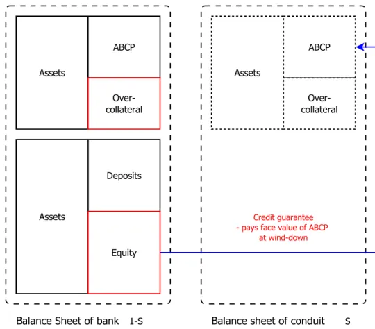
ABCP so that it attracts money market mutual funds: credit guarantees or liquidity guarantees. I denote the value function for the bank’s credit guarantee obligation asK(y), and the value function for the bank’s liquidity guarantee obligation as L(y). Under a credit guarantee, the sponsoring bank takes the conduit assets back and pay the ABCP investors its principal amount upon conduit wind-down: so the net transfer to the bank is−Pa+SVm(ya). I write the bank’s value function of
this payment asKw(y), so Kw(ya) =−Pa+SVm(ya). Figure 3 summarizes the capital structure of a bank structuring ABCP conduit with a credit guarantee.
Under liquidity guarantee, when the ABCP conduit winds down, the sponsoring bank pays the ABCP investor the fair value of the assetsSVm(ya), rather than the full principal amount. So the wind-down payoff function of liquidity guaranteeLw(ya) =−SVm(ya) +SVm(ya) = 0. The ABCP
investors are still subject to credit risk since the fair value of the assets underyamaybe lower than the par value of ABCP. Figure 4 summarizes the capital structure of a bank structuring ABCP conduit with a credit guarantee.
The high credit rating of ABCP relies on the credit or liquidity guarantee offered by the bank. Therefore, when the sponsoring bank defaults, the ABCP conduit has to be wound-down.16 In my model, the ABCP conduit is constructed such that ya ≥yb, so the conduit no longer exists when
the sponsoring bank defaults. In addition, I assume that when the conduit winds down and bank default happens at the same time, the residual of bank assets is always used to fulfill the bank’s credit or liquidity guarantee obligation before paying off the depositors. This is reasonable since the bank can always set the ABCP default barrier such that ya =yb+εso that the bank has to deliver the credit or liquidity guarantee before it pays its depositors.
Finally, the bank may not issue the full amount of underlying assets in the conduit as ABCP. Instead, the bank can only issue ABCP using a fraction of the assets, and holding the residual claim of the asset’s cashflow after the coupon of ABCP gets paid. When the cashflow from the underlying asset Syt is lower than the ABCP coupon payment kPa, the residual tranche needs to cover the cashflow shortfall. In addition, when the ABCP conduit gets wound down, the remaining
16
The existence of a wind-down trigger upon the sponsoring bank default does not conflict with the bankruptcy remoteness of the ABCP conduit as an special purpose entity. The ABCP conduit is still bankruptcy remote from the sponsoring bank since the creditors of the bank do not have claim to the assets in the conduit.
value of the underlying asset is used to pay ABCP investors only: the residual piece does not get any claim on the underlying assets. I assume that the sponsoring bank holds the residual on its balance sheet too.
3.1.2 Timeline
Figure 5 shows the timing of the events in my model:
At t= 0, the bank collects deposits and issues equity by determining the principal amountPd and interest rate c, such that the deposit is priced at par. The bank also uses ABCP funding. So the balance sheet contains 1−S fraction of the assets, and the bank moves S fraction of the assets into an ABCP conduit. The conduit sells asset-backed commercial paper with a principal amount
Pa and a coupon k to the investors. The bank equity holder invests in the residual claim, and offers a credit or liquidity guarantee to the conduit. The bank then uses the capital to originate the project. The social planner evaluates the risk of the deposits and charges the bank a one-time deposit insurance premium. The social planner decides the default threshold yb. The project then starts to operate.
At t >0, the following events may take place:
• The incumbent deposit or ABCP may mature: the bank (if still solvent) needs to pay off the
principal amount of the debt, and then reissues new debt under the cashflowytwith the same amount of principal. Since the cashflow yt may not be as high as y0, the new debt may be
issued at a discount since the investor may demand a higher return. In this case, the bank equity holder has to post the margin and will suffer a loss.
• The bank may exercise its one-time option to drop the monitoring on the project, and change
the cashflow dynamic.
• When the cashflow in the ABCP conduit hits the pre-specified barrierya, the ABCP conduit
winds down and the bank delivers its credit or liquidity guarantee to the commercial paper investor. The bank then liquidates the assets in the conduit.
• The social planner seizes the bank when the project cashflow hits the default barrieryb. The
social planner then creates a new bank that takes over the project the old bank’s assets at a discounted price that equals to 1−αfraction of the project’s liquidation value. The investors
get the liquidation value, as well as a reimbursement from the social planner for the loss of capital. The new bank then issues new sets of debts, and operates the project. Since the initial cashflow is yb, the new economy operates in a smaller scale yb/y0.
3.2 Benchmark Model with a Credit Guarantee
I first work on a benchmark case where the bank offers a credit guarantee to the ABCP. Since the social planner has no control over the bank’s shirking decision, the bank may choose to shirk from monitoring when it is in the bank’s best interest to do so. Suppose the optimal shirking strategy is to shirk at timeθ when the cashflow first hits the barrier yθ, so θ= inf{t:yt< yθ}. Then the
shirking will happen before the bank defaults if yθ > yb. I denote the value function for depositor asD(y), and the value function for bank equity holder as E(y). The value function of the social planner S(y) is the sum of the deposit insurance obligation I(y) and the tax income value T(y). Proposition 1 specifies the value functions in the benchmark model, assuming thatya=yb.
Proposition 1. Under the shirking barrieryθsuch that the bank will shirk at timeθ= inf{t:yt< yθ},
the value function for deposit is
D(y) =Pd,
the value function for the ABCP is
A(y) =Pa,
and the value function for the bank equity holder is
E(y) = (1−τ) [(1−φm(y;yθ))Vm(y) +φm(y;yθ)Vs(y)−P]
+ (1−τ) (P −Vs(yb))φm(y;yθ)φs(yθ;yb),
The value function of the social planner S(y) is the sum of the deposit insurance obligation
I(y) = [−P+ (1−α)Vs(yb)]φm(y;yθ)φs(yθ;yb),
the present value of the corporate income tax payment to the social planner is
T(y) = τ[(1−φm(y;yθ))Vm(y) +φm(y;yθ)Vs(y)−P]
+τ(P−Vm(yb))φm(y;yθ)φs(yθ;yb),
where φi(y;y0) is the state price of a unit payoff at the moment wheny first becomes smaller than
y0, when the project is under statei∈ {m, s}. Specifically,
φi y;y0 = 1 y0≥y y y0 Hi y0 ∈(y, y0] 0 y0 < yb ,
where y0 can either be yb or yθ, and
Hi= 1 2 − µi σ2 i − s 1 2 − µi σ2 i 2 + 2r σ2 i <0.
Figure 6 shows the value function of the bank equity holder under monitoring and shirking using a numerical example. When the cashflow of assets moves to the range in which shirking leads to a higher equity value, the equity holder will switch to shirking. In the following analysis, I assume the combination of model parameters ensures thatyθ ≤y0: in other words, the bank do not have
incentive to shirk immediately after the project starts.
I denote the total value in the economy as Σ(y). The total value in the economy not only contains the value of the social planner S(y), the debt holders D(y) and A(y), and the current bank equity holder E(y), but also the future total value of economy after the newly formed bank
takes over the current one. Hence, Σ (y) = D(y) +A(y) +E(y) +S(y) + [Σ (yb)−(1−α)Vs(yb)]φm(y;yθ)φs(yθ;yb) yθ> yb D(y) +A(y) +E(y) +S(y) + [Σ (yb)−(1−α)Vm(yb)]φm(y;yb) yθ≤yb .
Intuitively, since the monitoring keeps the value of project higher, the shirking option may introduce a moral hazard problem. Proposition 2 shows the total value function Σ(y), and the loss of total value introduced by the moral hazard.
Proposition 2. The total value in the economy is
Σ (y) = Vm(y)−φm(y;yθ) [Vm(y)−Vs(yθ)] yθ > yb Vm(y) yθ ≤yb ,
therefore the one-time option of shirking, which will be exercised by the bank in caseyθ > yb, causes
a loss of total value in the economyφm(y;yθ) [Vm(y)−Vs(yθ)]. So the bank’s shirking option does
introduce a moral hazard.
The moral hazard in the economy motivates a rational expectation equilibrium (REE), in which the social planner offers a continuous “menu” of the default barrier, given the amount of the bank’s deposit Pd and ABCPPa.
Definition. The rational expectation equilibrium is an equilibrium in which:
• The social planner commits to a default barrier of the bank yb, given the amount of deposit
Pd, and the amount of ABCPPa, issued by the bank. The social planner chooses the optimal
default barrier yb∗(Pa, Pd) to maximize the total value in the economy Σ(y). Among all the
choices ofyb that maximize the total value of economy, the social planner will pick the yb that
maximizes the bank’s total value at origination.
• The bank chooses the capital structure by deciding the amount of deposit issuance Pd and
ABCP issuance Pa, together with the default barrier of the ABCP conduit ya, to maximize
default barrier y∗b(Pa, Pd).
{Pa∗, Pd∗, ya∗}= arg max Pa,Pd,ya
v(y0;Pa, Pd, ya, yb∗(Pa, Pd)),
since the ABCP conduit will lose the P-1 rating once the guarantee becomes invalid, the bank is subject to a constraint
ya∗≥yb∗(Pa, Pd).
The following proposition shows that there exists a minimum exogenous default barrier, which varies with the bank’s debt, such that we can completely eliminate shirking by setting the default barrier strategically. Since sponsoring banks do not enjoy the “ABCP exclusion” when they provide credit guarantees to ABCP conduits, they have to prepare risk capital for the full balance of ABCP. This allows the social planner to implement the default barrier by enforcing a minimum level of capital ratio, when the capital ratioκ is defined as the book value of equity over the book value of assets
κ= Vi(y)−Pa−Pd
Vi(y) .
Proposition 3. In the rational expectation equilibrium, there exists an optimal default barrier yb∗
such that the bank does not shirk:
yb∗= P(Hm−Hs)
(1−Hs)/(r−µs)−(1−Hm)/(r−µm),
where P =Pa+Pd. The social planner can implement the optimal default barrier by enforcing a
minimum capital ratio
κ∗ = (1−Hs) (µm−µs) (Hm−Hs) (r−µs)
.
The total bank debt under the REE P∗ =Pa+Pd is
P∗= 1−κ ∗ r−µm (1−κ∗)τ (1−Hm) (α−κ∗τ) −Hm1 ,
and the bank chooseya∗ =yb∗.
decision directly, it can still solve the moral hazard problem by forcing an exogenous default barrier
yb∗, or equivalently a minimum capital ratioκ. Figure 7 plots the equity value functions under the minimum exogenous default barrier caseyb =yb∗: the shirking region has been removed.
Figure 8a shows the social planner’s best response y∗b to the bank’s outstanding deposits and commercial paper under REE. The linearity of the default barrieryb∗ shows that the barrier can be implemented by a minimum capital ratioκ∗. Figure 8b shows how the bank’s total value changes with the amount of deposits and commercial paper, given the social planner’s menu of y∗b.,
Two more results follow from the value functions and equilibrium default barrier. The value functions for the bank using deposit and equity only shows that the maturities of deposits and ABCP do not matter.
Corollary 4. The agents’ value functions remain invariant when the maturity m changes. Subse-quently, the REE equilibrium capital structure does not change with m either.
Deposit insurance makes the deposit riskless. Therefore, when the investors withdraw their deposits, the bank can always rollover the old deposit using new deposits priced at face value, even if the cashflow yt maybe lower than before. The credit guarantee to the ABCP plays a similar role and allows the bank to rollover the maturing ABCP without risk. The riskless rollover saves the bank equity holder from worrying about the maturity of debts since the equity value no longer changes with the maturity. Subsequently, the social planner, who tries to prevent the bank from shirking, does not need to consider the maturity when he is trying to set up the equilibrium default barrier. A maturity invariant default barrier also means the credit risk of the bank does not change with maturity. Therefore, the value of deposit insurance does not change with maturity as well.
The maturities of deposits and ABCP do not affect the equilibrium capital structure. Since all the agent’s value functions in the economy do not change with the maturity 1/m, the equilibrium does not move with the maturity.
Corollary 5. As long as the total amount of debt P =Pa+Pd is fixed, the value functions of the
equity holder and the social planner, as well as the default barrier yb, remain invariant when the
3.3 Model with a Liquidity Guarantee
Instead of using an ABCP conduit with a credit guarantee, the bank can also provide a liquidity guarantee to the ABCP conduit. Figure 4 shows the capital structure of a bank with a liquidity guaranteed ABCP conduit. The value functions are:
Proposition 6. The value function of ABCP is
AH(y) = k rPa+CHφm(y;ya). AL(y) = k+m m+rPa(1−ψm(y;ya)) +SVm(ya)ψm(y;ya)−CL ψm(y;ya)− ¯ ψm(y;ya) . where ψm(y;ya) = y ya Gm , ¯ ψm(y;ya) = y ya G¯m .
The coefficients Hi, i∈ {s, m}, is defined in Proposition 1,
Gi = 1 2− µi σ2 i − s 1 2 − µi σ2 i 2 +2 (r+m) σ2 i <0, ¯ Gi = 1 2− µi σ2i + s 1 2 − µi σi2 2 +2 (r+m) σ2i >0.
Finally, the CH, CL satisfies
AH(y0) = AL(y0),
A0H(y0) = A0L(y0).
The value function of the residual tranche investor is
R(y) = (1−τ) SVm(y)− k rPa(1−φm(y;ya))−SVm(ya)φm(y;ya) .
liquidity guarantee as a funding source, a change in maturity 1/mdoes change the value functions of the ABCP and the bank equity holder. In other words, the model shows that the maturity invariance property in the credit supported ABCP conduits no longer holds for the liquidity supported ABCP conduit. Figure 9a shows how the value of ABCP varies with its maturity, when ABCP receives a liquidity guarantee from the sponsoring bank. This motivates a careful study of the effect of maturity.
ABCP maturity 1/m Figure 9b shows that when the maturity of ABCP becomes shorter than a week, the credit guarantee and liquidity guarantee value functions are very close except for those cases with assets value close to the ABCP conduit consolidation threshold. In addition, even in the case wheny is close to ya, a shorter maturity means more risk remains on bank’s balance sheet.
Furthermore, the following proposition shows that when the maturity approaches zero, the liquidity support converges to credit support.
Proposition 7. When the ABCP maturity decreases, the liquidity support value function converges to the credit support value function. When the maturity intensity m→ ∞, Lr(y) =Kw(y) for all
y∈(ya,+∞).
The banking capital regulations before 2009 treated credit guarantees and liquidity guarantees differently. When the bank provides a credit guarantee, it had to have risk capital corresponding to 100% of the ABCP principal amount. The risk capital requirement for the bank that provides a liquidity guarantee, on the contrary, is only 10% of the ABCP principal amount. The ignorance of the intrinsic similarity of the credit guarantee and the liquidity guarantee for short-term ABCP gives us the false sense that the latter is much safer than the former. During the recent financial crisis, many banks that relied on ABCP as a funding source were forced to swallow huge credit losses that exceeds their risk capital. This finding also provides a theoretical support to the empirical finding in Acharya et al. (2012), which states that the ABCP sponsor bank kept the risk to themselves.
The value of a liquidity guarantee cannot be correctly measured without considering the ABCP maturity. The risk transferred out of the balance sheet will be higher during normal “nice” times.
However, once the cashflow deteriorates, the risk transfer becomes ineffective. Hence, the effort of determining a correct risk weight without considering the maturity is futile. More importantly, the capital regulation decision based on the risk transfer during regular times gives the banking industry false sense of security, as the next proposition shows.
Equilibrium What is the equilibrium capital structure when the social planner, under bounded rationality, imposes minimum risk capital ratio based on a conversion factor, which was 10% before the financial crisis, for the outstanding ABCP? I define the equilibrium as follows:
Definition. The bounded rational expectation equilibrium is an equilibrium in which:
• The social planner chooses the yb as in Proposition 3 by assuming a conversion factor ρ for
ABCP outstandingPa, so
y+b (Pa, Pd, ρ) =
P(Hm−Hs)
(1−Hs)/(r−µs)−(1−Hm)/(r−µm),
where P =Pd+ρPa.
• The bank then chooses the capital structure by deciding the amount of deposit issuancePdand
ABCP issuancePa, together with the default barrier of the ABCP conduit ya, to maximize the
total origination value v(y0), given the social planner’s optimal default barrier yb+(Pa, Pd),
Pa+, Pd+, ya+ = arg max Pa,Pd,ya v y0;Pa, Pd, ya, yb+(Pa, Pd) ,
since the ABCP conduit will have lost the P-1 rating once the guarantee becomes invalid, the bank is subject to a constraint
ya+≥yb+(Pa, Pd).
Intuitively, the social planner sets the default barriery+b for the bank, according to a belief that the bank only keeps aρ fraction of the risk for the underlying assets, instead of the full amount of risk as in a credit guarantee.
The capital structure under the bounded rational expectation equilibrium is different from the capital structure under the rational expectation equilibrium. Figure 10 shows the various principal amounts of ABCP and deposits under different values of conversion factor ρ, when the ABCP conduit is selling 90 day paper. Whenρbecomes smaller, the bank uses more ABCP funding. This result is due to the existence of conversion factorρthat did not fully capture the riskiness of ABCP, therefore allows the bank to use high leverage and shift the insurance burden to the social planner. Under the bounded rational expectation equilibrium, the equilibrium face amount of ABCP
Pa+ S >
Pd+
1−S,
whenρ is significantly smaller than 1, the equilibriumPd+is close to zero. In reality, banks usually move only the AA rated assets to the ABCP conduit for the rating purpose. Therefore, the actual capital structure decision between deposit funding and ABCP funding does not lead to a very small deposit funding. However, the intuition that the conversion factor incorrectly estimates the riskiness in ABCP funding and causes a distortion in capital structure, remains valid.
More importantly, when the maturity of ABCP changes after the capital structure has been fixed att= 0, the bank may default endogenously before yhits the default barrier imposed by the minimum capital ratio.
Proposition 8. When the maturity of ABCP m becomes very short after t= 0, then the default barrier y+b will not be binding. In other words, the bank equity holder will endogenously default when y hits some yˆb+> y+b , a.k.a. before the bank reaches the minimum capital requirement.
The proof is in the Appendix. The intuition is that, since the value function of the liquidity guarantee converges to the full credit loss amount when y → yb, while at the point yb the bank
is only responsible for the liquidation cost of non-defaulted assets. Therefore, the bank equity value function is discontinuous at yb, and there exists some εsuch thatE(y)< E yb+= 0, for all
y∈ yb+, y+b +ε
. The equity holder will choose to endogenously default before the cashflow hits the social planner imposed barrieryb+. This helps to explain why the major U.S. financial institutions with Tier-1 capital ratio way above the minimum requirement experienced sharp drops in share prices, and eventually shut down. Since the liquidity guarantee value function can have a large
negative rollover loss even before the ABCP conduit wind-down, the bank default can happen when the bank still has a higher than minimum capital ratio, and the ABCP conduit is still functioning. Thus seemingly healthy bank may collapse, causing big disruption in the economy.
4
Empirical Analysis
The theory section suggests that when the underlying asset deteriorates together with a decreasing ABCP maturity, the bank equity holder suffers more deficit by supporting the ABCP rollover. To test this hypothesis, I study how the ABCP maturity and the underlying conduit risk, as well as their interactions, drive the returns of banks that provide liquidity guarantees to the ABCP conduits.
4.1 Data and Summary Statistics
I focus on banks’ abnormal returns under different ABCP maturities and conduit exposures from April 2001, when FAS 140 became effective, to the end of 2009, when the “ABCP exclusion” was dropped. I use a variety of data sources to construct the sample used. The sample consists of data about the ABCP conduits and their guarantor banks, the credit information about mortgage loans, financial market conditions, regulatory policy dummies, and macroeconomic variables.
ABCP Conduit: Sponsoring Banks I collect the ABCP conduit information from Moody’s Investors Service, who publishes quarterly spreadsheets that summarize the basic information on most of the ABCP conduits. These spreadsheets contain the outstanding amount of commercial paper, the rating of the commercial paper, whether the conduit has a credit or a liquidity guar-antee, and the guarantor institution, for each ABCP conduit at each quarter end. Most of the guarantors are banks. Other types of institutions, such as asset management firms and automotive manufacturers, also provide supports to ABCP conduits: so I remove the entries for these conduits. Some mortgage lenders use ABCP conduits as mortgage warehouses to fund the newly originated mortgage loans that have not been moved into a mortgage pool for securitization yet. ABCP con-duits provide the working capital for these mortgage lenders: so I exclude these mortgage lenders. I also focus on the U.S. banks only. This leads to 18 guarantor banks in my sample.
Among the ABCP conduits, some of the them are CDOs that sell senior tranches as ABCP, while some others are Asset-Backed Securities whose senior tranches are commercial paper. I drop both types. Furthermore, some ABCP conduits have full credit guarantees as a repurchase agreement or a total return swap, which covers 100% of the ABCP balance, with a counter party other than the sponsoring bank. I drop these records since it is the total return swap protection seller that carries the credit risk.
I measure each bank’s quarterly absolute exposure to liquidity guarantees by aggregating the principal amount of outstanding ABCP across all the conduits supported by the bank in each quarter. I then normalize the exposure using the book value of the sponsoring bank’s balance sheet in the same quarter. In other words, the exposure for each bankiat periodtis:
Exposurei,t =
Total outstanding of ABCP that receives the guarantee Book value
i,t
The measure of exposure corresponds to the parameterS in my model. I repeat the same process to calculate each bank’s quarterly relative exposure to credit guarantee. The quarterly call reports also provides other balance sheet and income statement information, such as the tier-1 capital ratio, cash ratio, book value and earnings, which I use as control variables.
Daily returns of the commercial banks are from CRSP, which is also the source of the daily riskless rate and value-weighted index return with dividends. I dropped the records for the banks that have daily return lower than −20% or higher than 20%. I merge the daily returns of banks
with the latest quarterly ABCP conduit outstanding information as well as banks’ call reports before the return date.
ABCP Conduit: Underlying Assets It is difficult to obtain complete information about the assets in ABCP conduits, due to the nature of off-balance sheet financing. Nevertheless, Moody’s Investors Service does release, on an irregular basis, the mix of underlying assets for a few large ABCP conduits. In these conduits, a large fraction of the underlying assets are residential mortgage backed securities. Therefore, I collect the subprime mortgage delinquency information from ABSNet as a proxy of the expected future credit loss in ABCP conduit assets. Specifically, I focus on the
delinquency status of 30-year adjustable-rate subprime mortgages with a fixed rate for the first two years. Adjustable-rate subprime mortgages allowed the borrowers to enjoy a low teaser rate at the beginning, which initially made the mortgage loan more affordable than fixed-rate subprime mortgages. When the growth of home price began to soften in 2007, the subprime adjustable-rate Mortgage (ARM) borrowers started to show increasing level of delinquency. Since the borrowers with low credit quality usually do not recover once they are over 60 days delinquent,17the mortgage delinquency rate is a closely watched indicator of the healthiness of mortgage loans. I aggregate the monthly current balance of over 60 day delinquent subprime ARM 2/28 loans, and normalize it with the monthly total current balance of subprime ARM 2/28 loans.18 Figure 11 shows the change in subprime ARM 2/28 delinquency ratio during the study period.
Mortgage Delinquencyt=
Balance of over 60 day delinquent subprime ARM 2/28 loans Balance of subprime ARM 2/28 loans
t
.
The risk exposure of the sponsoring bank to ABCP conduits is the product of relative conduit exposure and the percentage of over 60 day subprime ARM 2/28 delinquent ratios:
Conduit Riski,t = Exposurei,t×Mortgage Delinquencyt
Commercial Paper Maturity I obtain both the Federal Reserve’s Asset-backed Commercial Paper and non-financial Commercial Paper market data for commercial paper maturity. The dataset includes the daily maturity distribution for newly issued ABCP and non-financial Commer-cial Paper. By summing up the issuance balance of the commerCommer-cial paper with different maturities, I obtain the distribution of maturity dates for the outstanding commercial paper.
I the use the ratio of the outstanding amount of ABCP maturing overnight to the total out-standing of ABCP with all maturities at the same period as a measurement for the overall maturity
17
There are two standard approaches to calculate days in delinquency: the Office of Thrift Supervision (OTS) standard, and the Mortgage Banker’s Association (MBA) standard. A mortgage loan that is 30 days delinquent in OTS standard is usually 60 days delinquent in MBA standard. Similarly, a 60 days delinquent loan in OTS standard means it is 90 days delinquent in MBA standard, and so on. The OTS standard has wider acceptance for subprime mortgage products. I follow the OTS standard in this paper.
18
The term 2/28 means the borrower will enjoy a low fixed teaser mortgage rate for the first two years, then a floating rate after that. The total term of the mortgage is 30 years.
of ABCP:
%OVNt=
Outstanding of ABCPs that are maturing overnight Total ABCP outstanding
t
A higher overnight share at day t corresponds to a shorter ABCP maturity, and also means the bank needs to deliver a large liquidity guarantee at that day. Since the parameter m in the model measures how fast the outstanding commercial paper hitting their maturity date, the share of ABCP maturing overnight is equivalent to the parameterm.
Figures 12a and 12b shows the daily fraction of ABCP and non-financial commercial paper maturing overnight. The maturity of ABCP shortened during the 2007 ABCP market freeze, while the maturity of non-financial commercial paper shortened during the 2006 downgrade of General Motors.
Other Macroeconomic and Financial Market Conditions I collect the macroeconomic data such as the monthly U.S. GDP and the magnitude of quantitative easing (QE). The GDP data is from Macroeconomic Advisers LLC, and the QE data is from the weekly mortgage backed security purchase amount published by the Federal Reserve. I also obtain general financial market conditions, including the market volatility from CBOE Dow Jones Volatility Index, the slope of treasury yield curve as the difference between 10-year and 3-month treasury constant maturity rate, and the spread between the Moody’s Seasoned Baa Corporate Bond Yield and 10-Year Treasury Constant Maturity Rate, all from the Federal Reserve Bank of St. Louis.
Table 1 shows the summary statistics.
4.2 Empirical Strategy
4.2.1 OLS Specification
My theoretical model suggests that the change in ABCP maturity impacts the risk transfer between the ABCP conduit and its liquidity guarantee providing bank.19 In other words, the interaction between the change in ABCP maturity and the change in ABCP conduit asset credit loss would
19Acharya et al. (2012) study the risk transfer in ABCP securitization using the following baseline specification:
change the sponsoring bank’s value. I estimate the effect of the interaction on the sponsoring bank’s abnormal return, a proxy of the change in bank equity value. As Figure 13 shows, a shorten ABCP maturity together with a drop in conduit value may cause the equity value to drop more.
Hence, my model implies the following specification:
rai,t = β0+β1×∆%OVNt×∆Conduit Riski,t +β2×∆Conduit Riski,t
+β3×∆%OVNt
+β4×Xi,t+β5×Yt+αi+εi,t.
Here rai,t is the holding period equity abnormal return of banki at periodt. For the explanatory variables, %OVNtmeasures outstanding ABCP during periodt, so ∆%OVNt measures the change in the ratio of ABCP outstanding matures overnight from period t−1 to t. ∆Conduit Riski,t is
the product of subprime mortgage delinquency rate change between periodt−1 andt, multiplies
the bank’s exposure to ABCP liquidity guarantee aforementioned, which is the principal of ABCP relative to the bank’s book value. The regression includes bank fixed effect αi to account for unobserved heterogeneity at the bank level that may be correlated with the explanatory variables. In addition, I control for bank balance sheet variablesXi,t, and macroeconomic variablesYt, both are discussed in the section 4.2.2. Finally, εi,t is a bank-specific error term. Standard errors are clustered at the bank level as well as at the year level to account for heteroscedasticity and serial correlation of errors as in Petersen (2009). My model suggests thatβ1 <0 given the fact that the
ABCP maturity modulates the risk transfer.
whereriis the cumulative equity return of bankicomputed over the 3-day period from August 8 to 10, 2007, and
ConduitExposurei,tis banki’s conduit exposure relative to total assets at timet. They find that, for those banks
that providing liquidity guarantees to ABCP conduits, a larger ABCP conduit exposure was associated with more negative stock returns during the short period of the ABCP market freeze. Acharya et al. (2012) challenge the belief that by transferring assets to an ABCP conduit and providing liquidity guarantee, a bank unloads the credit risk of those assets from its balance sheet.
4.2.2 Control for balance sheet, macroeconomic, and market variables
Banks can hold the same type of assets on their balance sheet as well as on the sponsored conduits. As a result, when the assets deteriorate, the bank return becomes lower even if the bank has completely transferred the conduit assets risk out to the investors. To control for this, I introduced the balance sheet information such as earnings per share as control variables to capture the losses on the balance sheet. Furthermore, other balance sheet variables, such as the cash ratio and the tier-1 capital ratio, may also varies with the bank’s exposure to ABCP conduit. Therefore I include them in the control variables as well. Finally, I also control for the bank’s exposure to credit guarantee. Bank specific controls are in theXi,t vector.
Macroeconomic and general market conditions can also change banks’ returns as well as the investor’s appetite to ABCP. Therefore, I control for the magnitude of the Federal Reserve’s quan-titative easing during the financial crisis by using the weekly mortgage backed security purchase amount. I also include the investor’s perceived volatility, a.k.a. the “fear index”, to control for the flight to safe assets during market turmoil. I also include the treasury yield slope to capture the difference between the short-term and long-term riskless rates. I control for the spread between Baa corporate bond and 10-Year treasury yield to capture the market’s changing risk appetite. I also control for the GDP growth as an indicator of general economy. The financial accounting standards for off-balance sheet funding channels have undergone changes in the 2000s: I have also included time dummies for FIN 46, and FAS 166/167. Yt contains these macroeconomic variables at periodt, as well as time dummies that account for different financial accounting standards.
4.2.3 Identifications and IV Specifications
The maturity of the ABCP conduit in the OLS specification is an endogenous regressor. The ABCP investor may choose to run or rollover to shorter term ABCP because the bank’s creditwor-thiness deteriorates, which is usually accompanied by a low excess or abnormal equity return of the bank. To see this, suppose the ABCP investors have time-varying intrinsic preferred maturity
IntrinsicM aturityt. They also adjust their maturity preference when investing in ABCP according to the bank’s current abnormal return. Then the change in the ABCP maturity for each bank i
becomes
∆%OVNi,t = ρ0+ρ1×∆Intrinsic maturity preferencet +ρ2×rai,t+ut,
which shows that ∆%OVNi,t is correlated withεi,t, therefore the estimated ˆβ0 and ˆβ2 are
inconsis-tent.
I use the following two identification strategies to tackle the endogeneity problem aforemen-tioned. First, the maturity of ABCP conduit may reflect the investor’s belief about the credit worthiness of the specific sponsoring bank. Using the average maturity of ABCP partly resolves this problem, since the idiosyncratic risk components among the banks can cancel out each other.
Second, I use the maturity of non-financial commercial paper as an instrumental variable. Many large non-financial firms issue commercial paper directly. These commercial paper have similar credit and liquidity profile as the ABCP, therefore, are usually sold to the same group of investors such as the money market mutual funds. The maturity of non-financial commercial paper correlates with the maturity of ABCP, since both of them are driven by the intrinsic maturity preference of investors. Similar to the ABCP, the non-financial commercial paper may also experience runs when the abnormal returns of the issuing firms are low. Therefore,
∆%OVN Non-financiali,t = θ0+θ1×∆Intrinsic maturity preferencet +θ2×ri,tN F,a+uN Ft ,
where %OVN Non-financiali,t is the maturity of non-financial commercial paper issued by firm i at period t, and the ri,tN F,a here refers to the abnormal return of the non-financial firm. However, the abnormal return of non-financial firms and the abnormal return of banks are orthogonal by construction. Therefore, I can use the maturity of non-financial commercial paper maturity as an instrumental variable, since the abnormal return of non-financial firms will not interfere with the estimation due to orthogonality. Figure 14 illustrates the identification strategy.
the change in average maturity of non-financial commercial paper as the instrumental variable. In thefirst stage, I estimate:
∆%OVNt = γ0+γ1×∆%OVN Non-financialt×∆Conduit Riski,t +γ2×∆Conduit Riski,t
+γ3×∆%OVN Non-financialt +γ4×Xi,t+γ5×Yt+αi+vt,
as well as the interaction term ∆%OVNt×∆Conduit Riski,t as the left-hand side variable in the
same first-stage setup.
In the second stage, I estimate:
rai,t = β0+β1×∆%OVNt×∆Conduit Riski,t +β2×∆Conduit Riski,t
+β3×∆%OVNt
+β4×Xi,t+β5×Yt+αi+εi,t,
where ∆%OVNtand ∆%OVNt×∆Conduit Riski,t are estimated from the first stage regressions. I
control for bank fixed effect. I also control for bank balance sheet variablesXi,t and macroeconomic variables Yt, as in section 4.2.2, in both the first and second stage regressions.
4.3 Results
4.3.1 OLS regression results
Table 2 shows the OLS regression result. Although the riskiness of conduits, approximated by the product of conduit exposure and subprime delinquencies, do not affect the bank’s excess return significantly, the interaction between maturity and the riskiness of the conduit significantly moves the sponsoring banks’ abnormal returns.
4.3.2 IV regression results
Table 3 shows the IV betas of the model presented in section 4.2.3. The result shows that the maturity of ABCP plays an important role. Although the maturity of ABCP, does not affect the bank’s return significantly, the interaction between maturity and the riskiness of conduit does move the return significantly.
Table 4 shows the first stage result. The relationship between the maturities of ABCP and non-financial commercial paper is strongly positive withp-value <0.01: when investors start to prefer shorter (longer) term non-financial commercial paper, they also start to prefer shorter (longer) term ABCP. The relationship is robust to the inclusion of bank fixed effect, macroeconomics control variable, and bank balance sheet control variables.
For instance, compare two banks, A and B, with identical conduit exposure at the average level 3.636% and both provide liquidity guarantee to a conduit with mortgage delinquency rate increases by 3.3 basis points, which is one standard deviation change. The empirical estimation result in Table 3 suggests that, suppose the percentage of outstanding ABCP with overnight maturity guaranteed by bank A is one standard deviation higher, i.e. 1.137% higher, than the percentage of similar outstanding ABCP guaranteed by bank B, the equity return of bank A will be 7.5 to 11.3 basis points lower than that of bank B. Therefore, regulators should consider the ABCP maturity as a critical factor when evaluating the riskiness of the ABCP conduit.
4.3.3 Robustness Test I: Excess Returns
To check the robustness of my regression result, I use bank excess return as an alternative measure of the sponsoring bank’s value. The OLS specification then becomes:
ri,t−rft = β0+β1×(rmt −r f t)
+β2×∆%OVNt×∆Conduit Riski,t
+β3×∆Conduit Riski,t
+β4×∆%OVNt
Here rtf is the riskless rate; ri,t is the holding period equity return of bank i at period t and
rtm is the market return at the same period, both calculated using the difference in the closing prices between periodtand t−1. In particular,rtm is the CRSP value-weighted index return with
distribution as the market return. Other explanatory variables and controls are the same as in section 4.2.1. My model suggests that β2 < 0 given the fact that the ABCP maturity modulates
the risk transfer. Table 5 shows the OLS regression result. The regression coefficients confirm that theβ2 is significantly negative, and the magnitude is close to the results obtained using abnormal
returns.
4.3.4 Robustness Test II: Maturity of Newly Issued ABCP
Testing the model using alternative measures of ABCP maturity further validates my empirical design and results. The ABCP conduit issues new commercial paper each day to replace to the matured paper. It issues more short-term paper when the investors demand shorter maturity. Hence an alternative measure is to compare the amount of overnight ABCP—with 1 day maturity—with the total outstanding of ABCP as of the previous day:
%OVN Issuancet=
Daily new issuance of ABCP with overnight maturity Total ABCP outstanding as of the previous day
t
,
and the %OVN Issuance Non-financialt is defined similarly for non-financial commercial paper. The overnight fraction of newly issued ABCP also subjects to the same endogeneity problem as in 4.2.3, and the similar identification strategy suggests a two stage least squares estimation (2SLS), with the change in overnight fraction of newly issued non-financial commercial paper as the instrumental variable. In the first stage, I estimate:
∆%OVN Issuancet = γ0+γ1×∆%OVN Issuance Non-financialt×∆Conduit Riski,t +γ2×∆Conduit Riski,t
+γ3×∆%OVN Issuance Non-financialt
+γ4×Xi,t+γ5×Yt+αi+vt,
in the same first-stage setup.
In the second stage, I estimate:
ri,ta = β0+β1×∆%OVN Issuancet×∆Conduit Riski,t
+β2×∆Conduit Riski,t +β3×∆%OVN Issuancet
+β4×Xi,t+β5×Yt+αi+εi,t,
where ∆%OVN Issuancet and ∆%OVN Issuancet×∆Conduit Riski,t are estimated from the first
stage regressions. I control for bank fixed effect, bank balance sheet variablesXi,t, and macroeco-nomic variablesYt, as in section 4.2.2, in both the first and second stage regressions.
Table 6 shows the IV regression result, using the alternative ABCP maturity measure ∆%OVN Issuancet. Again, the regression results are in line with the IV regression in Table 3. Table 7 shows the first
stage regression results.
5
Conclusion
The recent financial crisis challenged the effectiveness of conventional micro-prudential regulation. The adoption of various forms of shadow banking introduced complex risk transfers between a bank’s balance sheet and off-balance sheet entities. A careful study of these risk transfers is vital to the success of on-going regulation reform.
This paper studies the interaction between maturity transformation and moral hazard, under the context of banks financing through the off-balance sheet ABCP conduit. The deposit insurance isolates the maturity mismatch to the value function of depository institution equity holders, as well as the deposits, commercial papers, and the deposit insurance itself. Therefore, regulators can eliminate the moral hazard problem by imposing a simple minimum capital ratio requirement. For ABCP conduits with a liquidity guarantee, a change in the maturity of ABCPdoes affect the value function of the sponsoring bank. Therefore, the simple capital ratio rule without considering maturity mismatch is inadequate to solve the moral hazard problem. This result calls for more
comprehensive risk-based bank regulatory tests, especially stress tests that check the health of banks in adverse situations.