Country Report
Pro-poor Intervention Strategies in
Irrigated Agriculture in Asia
Poverty in Irrigated Agriculture: Issues and Options
India
Intizar Hussain, editor Study Team/Contributors:
MVK Sivamohan
Christopher Scott
Intizar Hussain
Bouma Jetske
Deeptha Wijerathne
Sunil Thrikawala
Hussain, I. 2004. (Ed.) Pro-poor Intervention Strategies in Irrigated Agriculture in Asia: India.
Colombo, Sri Lanka: IWMI. 204p. (Country report India)
ISBN Number 92 90 90 547 6
poverty / land resources / water resources / irrigation programs / institutional development /
institutions / organizations / irrigation management / water supply / water distribution / water
policy / financing / water rates / cost recovery / irrigation systems / irrigated farming / social
aspects / economic aspects / dams / constraints / river basins / catchment areas / soils / crop
production / cereals / public sector / employment / investment / dams / development projects /
water rights / legislation / privatization / water users’ associations / farmers’ associations / water
supply / indicators / irrigation scheduling / groundwater irrigation / water allocation
Contents
List of Tables and Figures
iv
Acknowledgement
vi
Study
Background
1
Part 1 – Poverty and Irrigation in India
1.1
Introduction
3
1.2
Historical
and
Contextual
Frame
4
a. Rural poverty in India
7
b. Water and land resources of India
18
1.3
Poverty Alleviation Initiatives in India – An Overview
26
1.4
Impact of Irrigation on Poverty – Review of Evidence
30
1.5
Performance of Irrigation Project – An Overview
42
1.6
Institutional Reforms in Irrigation
–
An
Overview
49
1.7
Summing
Up
57
Part 2 – Institutional Arrangements for Irrigation Management in India
2.1
Introduction
65
2.2
National-level Institutions for Irrigation Management
66
2.3
State-level Institutions for Irrigation Management
78
2.4
Local-level Formal and Informal Institutions for Water Supply
and
Distribution
106
2.5
Irrigation Financing: Water Charges and Cost Recovery
112
Part 3 – Poverty in Irrigation Systems – An Analysis for Strategic Interventions
3.1
Introduction
118
3.2
Study
Settings
and
Data
119
3.3
Poverty in Irrigated Agriculture: Spatial Dimensions
137
a. Socio Economic Features of Selected Systems
137
b. Poverty in selected Systems: Linkages and Spatial Dimensions
143
3.4
Determinants of Poverty in Irrigated Agriculture
155
3.5
Irrigation System Performance and Associated Impacts on Poverty
171
3.6
Analysis of Water Management Institutions: Implications for the Poor
181
3.7
Summary
and
Conclusions
188
List of Tables and Figures
Table 1.2.1. Rural Poverty Lit trends upto 1980 09 Table 1.2.2. River Basins in India 20 Table 1.2.3. Distribution of Soils 21 Table 1.2.4. Production and Yields of Crops 22 Table 1.2.5. Public Sector Investments in Irrigation 24 Table 1.2.6. Irrigation and Utilization 25 Table 1.4.1. Irrigated Agriculture and food grain production 33 Table 1.4.2. Per hectare production in different CAD projects 34
Table 3.2.1. River flows: Krishna basin 120 Table 3.2.2. Allocation of waters : Krishna Basin 120 Table 3.2.3. Sources of Irrigation 122 Table 3.2.4. Productivity of Principal Crops 122 Table 3.2.5. Plan-wise outlays in AP – Irrigation Schemes 122 Table 3.2.6. General features of the Command Areas 125 Table 3.2.7. Salient features of the selected irrigation system 126 Table 3.2.8. Area Irrigated : Harsi System 128 Table 3.2.9. Cropping Pattern : Harsi System 128 Table 3.2.10. Area under Irrigation: Harsi Command 129 Table 3.2.11. Area under Irrigation: Halali System 129 Table 3.2.12. Cropping Pattern: Halali system 129 Table 3.2.13. Selection criteria of villages selected for study 130 Table 3.2.14. Household sampling in Irrigation systems in AP 132 Table 3.2.15. Sample size for selected systems in MP 135 Table 3.2.16. Household sampling in irrigation systems in MP 135 Table 3.3.1. Types of houses in different project areas 137 Table 3.3.2. Facilities in housing premises in project areas 138 Table 3.3.3. Halali system – MP 139 Table 3.3.4. Harsi system – MP 139 Table 3.3.5. Nagarjuna Sagar Left Command – AP 140 Table 3.3.6. Krishna Delta System - AP 141 Table 3.3.7. Employment Pattern in the four Irrigation Systems 142 Table 3.3.8 . Income Poverty Indicators for the four systems 143 Table 3.3.9. Official Poverty figures for AP and MP 144 Table 3.3.10. Expenditure poverty indicators for the four systems 144 Table 3.3.11. Who are the poor in NSLC and KDS 145 Table 3.3.12. Who are the poor in Harsi and Halali 145 Table 3.3.13. Poor Vs Non-poor landholding households in NSLC and KDS 146 Table 3.3.14. Poor Vs Non-poor landholdings in Halali 147 Table 3.3.15. Poor Vs Non-poor landholdings in Harsi 147 Table 3.3.16. Correlation between different variables and poverty per capita – Halali 148 Table 3.3.17. Correlation between different variables and poverty per capita – Harsi 148 Table 3.3.18. Distribution of Poverty in NSLC and KDS- 149 Table 3.3.19. Distribution of Poverty in Harsi and Halali 149 Table 3.3.20. Agricultural production and farm income in NSLC 150 Table 3.3.21. Agricultural production and farm income in KDS 150 Table 3.3.22. Agricultural production and farm income in Halali 150 Table 3.3.23. Agricultural production and farm income in Harsi 151 Table 3.3.24. Distribution of Landholding size over the irrigation system 151 Table 3.3.25. Socio-economic indicators for marginal, small, large farmers in NSLC 151
Table 3.3.26. Socio-economic indicators for marginal, small, large farmers in KDS 152 Table 3.3.27. Socio-economic indicators for poor and non-poor farmers in
Halali and Harsi 153 Table 3.3.28. Average household expenditure on medicines and education in
Harsi and Halali 153
Table 3.4.1. Effect of Irrigation on Poverty in two systems – Irrigated and non-irrigated 156 Table 3.4.2. Effect of Irrigation on Poverty in two systems – head, middle and tail
of both systems vs non-irrigated 157 Table 3.4.3. Effect of Irrigation on Poverty in two systems- head and middle of both
systems vs Tail 158
Table 3.4.4. Effect of Irrigation on Poverty in two systems(MP)- irrigated vs
non-irrigated 159
Table 3.4.5. Effect of Irrigation on Poverty in two systems(MP) - head, middle
and tail of both systems vs non-irrigated 160 Table 3.4.6. Effect of Irrigation on Poverty in two systems(MP) - head, and middle
of both systems vs tail 161 Table 3.5.1. Productivity , equity and water supply indicators for the four irrigation
Systems 172 Table 3.5.2. Productivity , equity and water supply indicators for the four irrigation
systems in AP (reach-wise) 173 Table 3.5.3. Economic, financial, environmental and infrastructure sustainability
Indicators 175
Table 3.5.4. Economic, financial, environmental and infrastructure sustainability
indicators in AP (reach-wise) 176 Table 3.5.5. Institutional\Organizational \Management effectiveness indicators
for the four irrigation systems 176 Table 3.5.6. Institutional\Organizational \Management effectiveness indicators
in AP reach-wise) 177
Table 3.5.7. Water charges and collection in AP 178 Table 3.5.8. Crop Productivity before and after PIM 179 Table 3.5.9. Assessment of Impact of PIM 179
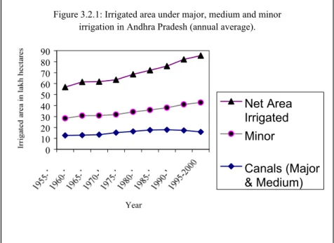
Figure 1.2.1. Change in Rural Poverty 1983-2000 17 Figure 1.2.2. Change in Urban Poverty - 1983 – 2000 17 Figure 2.5.1. Structure of the Irrigation Department 114 Figure 2.5.2. Structure of the Department of Water Resources 115 Figure 3.2.1. Irrigated area under major , medium, and minor irrigation in AP 123 Figure 3.2.2. Schematic map showing major and minor distributaries in KDS 133
Acknowledgement
We are thankful to Dr Kishor Goswami who worked as research analyst on the project for a short term for meticulously crosschecking the survey data and calculating poverty figures in Andhra Pradesh (AP). Thanks are due to several government officers in AP and MP (Madhya Pradesh) for providing support during field work and all the level officials, academia, NGOs and representatives of farmers who interacted with the study teams at different points of time. Thanks are also due to all the librarians, government officials and academia who helped us in identifying literature sources and other documents. We are thankful to Dr. Ranjitha Puskur, Special Project Scientist, IWMI, for her valuable suggestions in the preparation of this report. Contribution from Deeptha Wijerathne and Sunil Thrikawala in quantitative analysis is also gratefully acknowledged. This work is carried out in collaboration with national partners, SRIJAN in Madhya Pradesh and IRDAS (Institute of Resource Development and Management) in Andhra Pradesh. We are thankful to Mr. P Narayana, Mr. M Surender Reddy and Mr. B Ram Kumar for their help and comments. Ms. R Navanitha, apart from providing secretarial assistance, provided help in analysis of data. We record our deep appreciation and thanks to her.
Study Background
Agriculture in India as a whole has made remarkable progress over the past three decades. The average annual growth recorded in agriculture and allied sectors (forestry, and fishing) during the post reform years 1992-93 to 1999-2000 was 3.9 percent compared to 3.6 percent in the period 1980-81 and 1991-92 (at 1993-94 prices). Even if growth in food grains, the most dominant segment of crop agriculture, decelerated from 2.9 percent to 2 percent in the post reform period (while population growth rate is 2.1 percent, according to the population census of 2001), there has been a high growth maintained in wheat (3.6 %) and even rice (2.2 %) leading perhaps to the problem of excess stock of food grains (nearly 44 million tons). Robust growth in food grains production, despite below-normal rainfall in some regions, characterized 1999-2000, yielding a record food grains output of 208.9 million tons (GoI 2001). During the last 10 years (1990-2000), food grains area has ranged from 123 million hectares to 130 million hectares, the inter-year variation being influenced by weather conditions.
Despite these achievements, the productivity of a large part of irrigation systems remains severely constrained by inadequacy of some or all inputs. Such low-productivity areas are characterized by persistent rural poverty. The distribution of the benefits from irrigation development is thus largely skewed and unequal. While the determinants of low productivity are numerous and complex, they are to a large extent associated with poor performance of many of the established irrigation systems, which causes low, inequitable, and unreliable water supplies in those areas1.
The overall goal of irrigation development in India has been the improvement of national food security, rural and agricultural development and economic growth. Starting from the First Plan period, huge investments in canal irrigation have been made to achieve these objectives and important results were no doubt obtained. Irrigation has become the ‘prime engine’ in agricultural production and significant strides have been made in poverty reduction. Yet, entrenched pockets of poverty persist in many states, which raises serious questions about intervention strategies in the face of systemic poverty. Though the importance of irrigation is well recognized by several studies, irrigation-poverty linkages have not been studied in a greater depth.
However, over a period of time it is increasingly felt that investments in irrigation systems alone were not enough; the management of systems was crucial too. It became apparent that the operation and maintenance of the irrigation system and allocation of available water largely determine irrigation performance and the extent to which the objectives of irrigation development are being met. Research has shown that in India, irrigation performance of large and medium scale irrigation projects in general, has been poor. Historically, these systems have been managed by the state with little participation of the users. Irrigation administration has become highly centralized and supply-oriented at the discretion of government agencies. In order to improve irrigation performance in India, irrigation sector reforms have been taken up since the last decade, decentralizing management and devolving power to the users concerned. The effects of these changes on the efficiency and equity of water use are not yet clear: especially with regard to poverty, the linkages between irrigation performance, management reform and poverty alleviation have hardly been assessed.
1 Low-productivity regions are located largely in the tail- end areas of government-managed irrigation systems in most parts of
India. However, the level of poor performance varies from Bihar and Uttar Pradesh to the Krishna Delta System in Andhra Pradesh and Vishweshwaraiah Canal System in Karnataka.
Objective
The overall goal of the proposed study is to promote and catalyze equitable economic growth in rural areas through pro-poor irrigation interventions in the participating DMCs (including Bangladesh, the People’s Republic of China [PRC], India, Indonesia, Pakistan, and Vietnam). The immediate objective is to determine what can realistically be done to improve the returns to poor farmers in the low-productivity irrigated areas within the context of improving the overall performance and sustainability of the established irrigation schemes.
This report synthesizes the findings of a two-year study in India focusing on the states of Andhra Pradesh and Madhya Pradesh as part of a six-country research project led by the International Water Management Institute (IWMI) and supported by the Asian Development Bank. The central research issues in this context are “whether and to what extent irrigation development and past irrigation management practices have contributed towards achieving the broader goal of socio-economic upliftment of rural communities, and if it has not, then, what are the causes of under-achievements and how have these affected the lives of the poor in rural agricultural communities.”
In order to ensure comparability of results and findings across six countries and diverse contexts within countries, the following hypotheses were framed at the inception of the project:
1. Command areas of specific canal reaches receiving less irrigation water per ha have lower productivity and a higher incidence of poverty.
2. Under existing conditions, small, marginal and poor farmers receive less benefits from irrigation than large and non-poor farmers.
3. The greater the degree of O&M (Operations and Maintenance) cost recovery the better the performance of irrigation management.
4. Effective implementation of PIM/IMT (Participatory Irrigation Management/Irrigation Management Transfer) leads to improved irrigation system performance, which in turn reduces poverty.
5. An absence of clearly defined water allocation and distribution procedures, and absence of effective and clear water rights (formal and informal) adversely affects the poor more than the non-poor.
6.
There is scope for improving performance of irrigation systems under existing conditions,with
effective and improved institutional arrangements.
Elaborate framework for research was developed and the conceptualization and work plan was developed for the six-country study by IWMI2. The national partners were advised to follow the guidelines with some modifications as suitable to specific country contexts. These were further refined through a series of workshops at national level and a regional workshop.
The focus of the study was on selected representative low productivity irrigated areas with an emphasis on identifying and assessing a set of appropriate economic, financial, institutional governance and technical interventions at field and system levels and framework as far as they affect the poor’s access to water resources.
The study employs both qualitative as well as quantitative methods of analyses though the emphasis is on in depth quantitative analysis.
2
See International Water Management Institute (2001) Inception report and draft work plan, IWMI, Colombo (mimeo).
Part—1
Poverty and Irrigation in India
1.1 Introduction
1.2
Historical and Contextual Frame
a. Rural poverty in India
b. Water and land resources of India
1.3
Poverty Alleviation Initiatives in India – An Overview
1.4
Impact of Irrigation on Poverty – Review of Evidence
1.5
Performance of Irrigation Project – An Overview
1.6
Institutional Reforms in Irrigation – An Overview
PART I
Poverty and Irrigation in India
1.1. INTRODUCTION
In spite of a substantial natural endowment of water resources in India, their utilization has remained un-even. The country as a whole is likely to reach a state of water crisis before 2025, with significant water scarcity being experienced already in some regions of the country. The economy is no longer predominantly dependent on agriculture, yet, about two-thirds of the population living in rural areas do depend on it for their livelihood. Irrigated agriculture in this context has become the ‘prime engine’ of agricultural production. Paradoxically, food grains surplus co-exists with chronic and absolute poverty. Significant strides have been made in poverty reduction both in rural and urban areas. However, entrenched pockets of poverty persist in many states which raises serious questions about intervention strategies in the face of systemic poverty.
This part of the report is in the nature of a literature survey to establish the present state of knowledge on the impact of irrigation/management on poverty, with a specific focus on irrigated commands of major and medium irrigation projects in India. This forms the first foundation component of the study.
The literature review examines previous studies on impacts of irrigation/management on poverty, and linkages between irrigation and poverty in the background of a wider canvas. While doing so, a discussion on water-related institutions, policies, regulations, water charges and recovery, water related laws are not included as they form a substantial part of the second foundation component of the studies on institutional arrangements for irrigation management in India.
The literature survey is based on published and mimeographed materials collected from several libraries and state governments and government of India offices. Interactions with a number of government officials and researchers helped us in organizing the report and synthesising diverse aspects in a coherent fashion.
1.2. HISTORICAL
AND
CONTEXTUAL FRAME
The early history of the Indian economy, ever since the colonial rule roughly through the first half of the post-independence period, was punctuated with recurring famines, droughts and floods. ‘Vagaries of monsoon’ was the explaining phrase for fluctuations in GDP. From 1970 onwards the scenario changed as the Indian economy was no longer prominently driven by fluctuations in agricultural GDP. Bad rainfall years in 1987-88 and 1991-92 did not negatively affect the GDP unlike the earlier drought years (1957-58, 1965-67, 1972-73 and 1979-80). This trend to a great measure was a result of the extensive irrigation infrastructure created in the country through massive investments, and also because of the dwindling influence of agriculture itself on the GDP. The share of agriculture which stood at 55 percent of the GDP in 1950, had dropped to 26 percent in 1999. The GDP growth rate of 3.5 percent per annum before 1973-74 improved to 5 percent per annum thereafter indicating better economic performance in the latter half of the post-independence era. However, this does not undermine the crucial importance of agriculture in the Indian economy. Though lagging behind some of the Asian ‘Tigers’, India has made impressive strides in the agricultural sector and achieved self-sufficiency in food grains production. Agriculture is still the mainstay of 60.23 percent of the population living in rural areas and it will continue to be so. Fully 46.66 percentof the rural population is self-employed in agriculture and allied activities and 13.5 percent are agricultural laborers. However, there is inter state variation among the rural poor: 38.5 percent come under self-employed in agriculture followed by 23.32 percent agricultural laborers (Pant and Kakali 2001). Thus agriculture still contributes to the lion’s share of total employment in India. Dandekar(1981), holds the view that the growing disparity between agriculture and non-agriculture sectors in per capita GDP arises primarily from the structural features of the Indian economy. Despite this disparity the population does not move from agriculture to non-agriculture. “Agriculture is the parking lot for the poor” in India (Dandekar 1994).
Growth and equity are well-recognized objectives of national policy as reflected in the Five Year Plan documents and policy statements. However, one of the most hotly debated issues in the Indian context has been whether the growth process has actually benefited the poor (Panda 2000). The theoretical and empirical explorations in development studies have long engaged the attention of academia on the distributional aspects of economic growth. This was sought to be understood in terms of the inter-relationship between economic growth, income inequality, poverty and welfare among the various regions and the constituent socio-economic groups at the national and international levels. Abundant literature on poverty-related aspects thus sprang up both at macro and micro levels. The literature on poverty-related issues can be broadly classified into four overlapping time periods: i) the initial decades of independence up to 1968, ii)the green revolution period up to 1980’s, iii) the pre-economic reform decade of 1980-1990 and iv) the post pre-economic reform period from 1991 onwards. Contextual developments in the country, to an extent also, prompt segregation into these four periods during which the literature on poverty-related issues had continued to evolve. In the initial period, studies on inequality and poverty had a major focus on the aspects of measurement. Rich statistics have been accumulated on income and consumption ever since the National Sample Survey (NSS) started collecting data. Several of the studies were based on NSS data during that period but had to make necessary adjustments for estimation. Social scientists joined the fray by measuring poverty based on per capita calorie requirements. On the socio-economic front the thrust in the initial years was on institutional and agrarian reforms as well as expansion of the agrarian base. The principles of ‘Democratic Socialism’ saw
greater degrees of state intervention for the welfare of the people. The zamindari (landlord-tenant) system and the intermediary tenures, which existed during that time covering 40 percent of the cultivated area were abolished. Tenancy Laws were enacted in several states providing security of tenure to the tenant. Roughly two million agricultural co-operatives came into existence and the credit provided by them increased from 8 percent of total borrowings of cultivators in 1950 to 30 percent by the mid-1960’s (Radhakrishna 1993).
However, during this period the underlying trend of growth remained modest and was based more on area expansion than on improvement of yield. While the gross irrigated area increased from 22.6 million hectares (m ha) in 1950-51 to 32.7 m ha in 1966-67, the fertilizer consumption per hectare – an indicative index of technological change – was only 7 kg per hectare in 1966-67 (Rao 1996). By this time several studies on poverty attempted to determe the number of people below the poverty line (BPL) based on income or consumption. Ahluwalia (1978) examined the trends in the incidence of poverty for 14 different years for the time period 1956-57 to 1973-74 for India as a whole and for individual states. He adopted both Sen’s poverty index (Ps) and the traditional head count method in his analysis. Though a significant time trend was not visible, he found a statistically inverse relationship between rural poverty and agricultural performance for India as a whole. The same relationship was also observed in different states.
The next period up to 1980 was broadly the phase of the ‘green revolution’, which started in 1965 and continued through the early 90’s. Following Kuznet’s findings that income equality takes an inverted ‘U’ shape as the economy grows, some scholars claimed that the poor hardly gained from the ‘green revolution’, while many others found evidence of the “trickle down” phenomenon. Evidence on the distributional changes accompanying growth is mixed, but historical evidence for a number of countries shows only gradual change over fairly long periods. In India, the income gini coefficient remained almost constant from 1951 through 1992, with a mean of 32.6 and standard deviation of 2.0 (Li et al. 1998). The sectoral composition of growth also makes a difference for poverty reduction. Ravallion and Datt (1996) provide evidence for India that faster agricultural growth is strongly and unconditionally associated with both urban and rural poverty reduction.
Lipton and Longhurst (1989) cite the example of Indian Punjab to illustrate the dramatic transformations that have occurred with the widespread adoption of green revolution technologies. They opine that modern varieties do reach small farmers, reduce risk, raise employment and restrain food prices. Yet, the benefit in terms of poverty reduction appears to be modest. They observe that the poor are increasingly land-poor and dependent on wage labor. They argue that the benefits to the poor as consumers, (low food prices) are captured largely by their employers, who can pay lower wages. The green revolution phase was signified by desperate attempts to make a breakthrough in domestic food production. With the spread of high- yielding varieties, agricultural production showed a dramatic upward trend from 24 million tons in 1950 to 31 million tons in 1966, 43 million tons in 1972 and further 54 million tons in 1979. The gross irrigated area increased from 33 m ha in 1967 to 52 m ha in 1984 and over the same period, fertilizer consumption increased from 7 kg / ha to 45 kg / ha.
Rural poverty in India declined from 56.44 percent in 1973-74 to 53.07 percent in 1977-78. In the 70’s, strategies for poverty eradication were part of a larger belief in the importance of ‘growth with redistribution’. The production cum technology approach was supplemented by several interventions by the government to provide food and employment security to the poor. However, they remained as modest relief measures. In spite of wide ranging interventions and the green revolution, the poor appear to have
continued under considerable economic pressure. The per capita annual availability of food grains remained at 161 Kg during 1976-80 like in 1956-60 (Rao 1996). Although technology made an important difference for poverty reduction it was not the only contributing factor. Institutional change, sometimes responding to technological change and sometimes to government policy or social pressures, was also important. (Bussolo and O’Connor 2002).
From the early 1980s’ phase of fiscal belt-tightening and interventions, the policy moved away from redistribution and basic needs towards structural adjustments and market-oriented economies. Poverty as such was given a relatively low priority during the 1980s (Gita Sen 1999). There is ample evidence to show that the rate of decline of poverty was higher in the 1980’s than in the 1970’s. This can be attributed to higher growth in agricultural production, slower growth in food grain prices and the presence of safety nets. The safety nets are in the form of drought and flood relief programs (during the years of natural calamities) and the public distribution system (PDS) for basic commodities during the 1980’s. The GDP growth rate increased to 5 percent in the 1980s when an expansionary fiscal policy was adopted together with limited trade liberalization. However, this could not be sustained for long and led to a major balance of payments crisis in 1991. The crisis during 1991 arose out of excessive public spending and large and inefficient public sector functioning during the 1980s. Gaurav Datt (1999) estimates a mixed picture of moderate decline in urban poverty rates, but relatively unchanging levels of rural poverty after the economic reforms from 1991 onwards, which he surmises was because of a differential growth in average living standards in urban and rural areas. After 1993-94 not many studies on poverty are available. However, the latest official statistics shows that rural poverty is coming down compared to urban poverty in states like Andhra Pradesh. Detailed literature review on poverty and irrigation is presented in the following sections.
1.2A. RURAL POVERTY IN INDIA
Poverty is an age-old phenomenon in the Indian sub-continent. Evidences on Poverty in India in the late 18th century and 19th century vividly portray the then existing socio-economic environment and the mercenary impact of alien rule in accentuating the poverty of the masses. However, rigorous estimates on poverty started after independence. “It took 20 years for the national poverty rate to fall below – and stay below – its value in the early 1950s” (Revallion and Datt 1996). However, the absolute number of poor in the country still remains high accompanied by glaring regional imbalances.
A quick review of literature on rural poverty in general cannot be avoided here for, aspects of irrigation, agriculture and poverty are significantly embedded in the researches on rural poverty in India.
i) Early decades of independence upto 1968
There are two literature surveys on rural poverty related to the time periods of early decades of independence upto 1968 and the other upto 1980s. The first one is on poverty, income distribution and development (Sastry 1980) and the second on rural poverty (Thakur 1985). In the introduction, Sastry traces the debate on development, economic growth, income distribution and inequality in different countries and sets the stage for the literature survey on income and expenditure inequality in India. In the absence of official figures on income distribution in the early stages, several organizations and individual scholars tried to arrive at the pattern of distribution on a wider base. Some of them were based on consumer expenditure (from National Sample Survey (NSS) data) and others defined size distribution of personal incomes based on some simple hypotheses on saving behavior.
Absolute poverty adopting an objective boundary line called the BPL (below poverty line) became the frame of reference for several empirical studies measuring poverty. The BPL is defined in terms of per capita household consumer expenditure. Some of the important studies in this context often quoted are by Minhas (1970), Tiwari (1968), Ojha (1970), Dandekar and Rath (1971), Bardhan (1979). Minhas was criticized for underestimating the poor falling below the poverty line by excluding the expenditure on health and education. Dandekar and Rath’s study became controversial because of the revisions they made to NSS Consumer expenditure data of 1967-1988, and also for their use of national income deflator for the conversion of current price data into 1960-61 prices. Dandekar (1981) pointed out that their study of 1971 used the classification of the household on the basis of per capita monthly expenditure for calculating incidence of poverty, and not per capita caloric availability which was linked to the assessment of under nutrition. Ever since 1970s India has been predominantly concerned with income poverty. This began with the working group (GOI 1962) of economists set up by the Government of India to decide the extent of poverty in the country. It set the trend for defining and measuring poverty by using either income or consumption.
A brief annotated reference of some of the important studies pertinent to the period 1950s to 1980s is given in table. 1.2.1. The literature survey shows that the concern of researchers was more on ‘measurement’ and ‘methodologies’ for estimating poverty. While measuring poverty in the early decades, the regional variations were not taken into account by researchers in estimating prices of food items and other requirements.
In the 1950s and 1960s development was viewed as linked to high rates of growth in aggregate and per capita incomes by national leadership as well as aid-giving agencies. While attempting reformatory measures like abolition of Zamindari system, tenancy legislations, etc., during the First Five -Year Plan period, agriculture got a clear policy direction which to an extent benefited the poor. However, ‘trickle down’ theory fortified the approach of aggregate growth. The assumption was that reduction of poverty could only be tackled after a certain level of attainment of GDP (Graffin 1976).
Table 1.2.1 Rural Poverty: Literature trends upto 1980.
Study topic (author/year) Study objective: key research issues/questions explored
Hypothesis tested Summary of findings/conclusions List of recommendations Early decades of Independence upto 1968
Poverty and economic development (Sen 1975); Poverty in India: then and now 1870-1970 (Dantawala 1973); The writings of Dadabhai Naoroji, Karl Marx, RC Dutt, GU Joshi, AO Hume and Digby; see Indian economic through: Nineteenth century perspectives (Ganguly 1977), towards a reinterpretation of nineteenth century Indian economic history (Morris 1968)
The debate on Indian poverty in the 19th century brought out the socio-economic conditions of the time and mercenary impact of alien rule in accentuating the poverty of the masses.
Study Group 1962 – Fixation of per capita consumption in India
The study group recommended Rs. 20/- per month at 1960-61 prices (excluding expenditure on health and education) as per capita consumption. This was adopted as the poverty line.
The inequality of Indian incomes (Lydall 1960)
Estimation of distribution of income for the year 1955-56
Assumed that Pareto Law of distribution applies to India like most other countries.
The exercise was conducted by linking income tax data with consumer expenditure figures from NSS data.
By comparing the pre- and post- fractile shares of In income tax in India with UK concludes that the final distribution of real income is a good deal more unequal in India.
A note on the derivation of size distribution of personal household income from a given size distribution of consumer expenditure (Iyengar & Mukeherjee 1961)
Estimation of distribution of household income for the years 1951-52, 1943-54,1956-57
Used NSS data ad data from RBI for estimations. The conclusion was that the top 10% and bottom 50% of population increased their share in total income. Inference was that the position of middle income group worsened.
RBI study (1963) Analysis of income structure in three groups of household with different income structure
Unrelated data from different sources used to build a meaningful pattern. Relied on integrating NSS and RBI data
Contrary to general impression, the degree of inequality in income distribution in India was not found to be higher than in some advanced countries.
It was at variance with other empirical studies conducted before. Criticized for lack of concept, incorrect use of NSS data, methodological errors, (the equity of Indian incomes in India, Ranadive 1965)
Patterns of income distribution and savings (Lokanathan 1967)
Size distribution of income for the country as a whole was estimated. Study income distribution was conducted in 1960 and study on savings in 1962 and both were put together
Results of the two studies showed that upto 1% of the rural households had a per capita income which was 12 times the per capita income of the poorest 5% of the households. A similar pattern was observed for urban areas also.
Pattern of income distribution in India 1953-54 to 1959-60 (Ranadive 1968)
Study on trends in income distribution Kuznet’s hypothesis 1.The income structure in India is comparable to that in other under- developed countries. Greater income inequality observed in India also compared to developed countries. 2.Ten years of planning had no impact
on the income tax structure narrowing inequalities.
Distribution of Income: Trends since Planning (Ranadive 1971) mimeo as quoted in (Sastry 1980)
Estimation of various measures of inequality for income and consumption expenditure
Measures of inequality covered were (i) the concen-tration ratio (ii) standard deviation of logarithms (iii) Co-efficient of variation and iv) share of lower and higher deciles
The study covered income and expenditure separately both for rural and urban areas separately.
A configuration of Indian Poverty. Inequality and levels of living (Ojha 1970)
Poverty Estimations Adopting calorie norm of Rs. 2,250 per capita, the study assumes 66% of the calories obtained from food grains, cereals and pulses in urban areas and 80% in rural areas.
The study looks at both rural and urban poverty for the year 1960-61 and at rural poverty for the year 1967-68.
Concludes that 70% of the rural population for the year 1967-68 were below the level of minimum food grain consumption. The study excluded expenditure on health, education and housing. Poverty in India (Dandekar 1971)
and Nilakanth Rath .
Estimation of poverty, review of developments and future projections and policies.
Used NSS data without corrections. Asserts that the growth of economy was slow and small gains of development were monopolized by richer sections. Cautioned at the possible widening gulf between rich and poor.
It was estimated that in 1960-61, about 33.12% of rural population and 48.64% of urban population lived on diets inadequate in terms of calories. Rich have to bear the burden if solutions to poverty are viewed from the framework of private property.
On the minimum level of living of rural (Bardhan 1970).
Estimation of poverty Time series profile of the rural and
urban poor showed a sharp rise in incidence of poverty over time.
The findings were in contrast to those of Minhas,. Main objection to the study was for using agricultural labor consumer price index for deflating the consumption of rural poor.
Rural poverty land distribution and development (Minhas B S 1974)
Estimation of poverty. Based on figures recommended by 1962
study group. Estimated that the poor decreased from 173 million in 1956-57 to 154 million in 1967-68. He took lower figure of Rs. 200 per annum (BPL) for rural population.
Expenditure on health, education were not taken into account and hence the estimates were criticized as under estimates.
Inequality and poverty in rural India (Bhatty 1974).
Incidence of poverty among different rural occupational groups.
Adopting both Sen’s poverty index and also the head count quantified incidence of poverty at different levels of per capita monthly income at 1968-69 prices. The study used survey data of National Council of Applied Economic Research.
Shows that the incidence of poverty is severe among agricultural laborers and least among non-agricultural work force in villages.
Estimates of population figures of BPL were lower like Vaidyanathan’s (1974), when compared to Dandekar & Rath (1971) Minhas (1970) and Ojha (1970).
Poverty in rural India: A decomposition analysis (Padmaja Pal et. al 1986).
Assessing incidence of poverty among different sections of population in rural India.
Based on 28th round NSS household budget data relating from October 73 – June 74.
The contributions of different categories to the overall poverty in rural areas were computed using head count ratio and as decomposable units as worked out by Chakravarthy (1984).
ii) The Green Revolution period upto 1980
It was argued by Tyagi (1982) that, the estimates of poverty during 1960’s were ‘overestimates’ which got moderated over the years and they cannot be taken at their face value. His analysis cautioned against the erroneous tendency to arrive at conclusions in establishing the relationship between the trends in rural poverty and agricultural growth in the country based on such figures. Contrary to what was deduced from NSS data by some experts, agricultural growth certainly had a positive impact on rural poverty. The spectacular success of green revolution and the mounting evidence of its short-term and long-term impacts, which was clearly perceptible during that period, drove the policy makers to focus on technology-based strategies thereafter. The production cum technology approach to agriculture supplemented by various policy measures like food and employment security to the poor, several targeted and area development programs improved the economic scenario of the country. Income poverty declined significantly between the mid-1970s and end 1980s, the period when India had a higher and stable trend rate of agricultural growth. Interestingly, green revolution could not however bring in higher growth rates of different crops except wheat and rice. In fact, the growth rates were less in post-green revolution period (1966-85) than in the pre-green revolution times (1950-65) Hanumanth Rao et.al ,(1988) attribute this trend to the fact that green revolution was effective with only some high yielding crops confined to some areas and was unable to compensate for the slowing down trend in the expansion of area under crops. The green revolution has helped agricultural growth undoubtedly, but government initiatives were not commensurate with growth to distribute the benefits equitably. Its impact was first felt in the states of Punjab, Haryana and Western Uttar Pradesh and later on gradually spread to the southern states of Andhra Pradesh and Tamilnadu.
Researches on poverty continued during this period bringing in more refinements in measurement and tools. Two of the important time series studies during this period were by Ahluwalia (1978) and Dutta (1980). The paper by Ahluwalia establishing relationship between rural poverty and agricultural performance, triggered off several empirical researches on the subject. Inverse relationships were observed in between the two variables, thereby asserting the ‘trickle down’ mechanisms. Based on the evidence from all over the country the findings of Ahluwalia’s study were as follows:
a. No discernable trend observed between 1956-57 and 1973-74.
b. Reduced incidence of poverty was associated with improved agricultural performance measured as an increase in the net domestic product in agriculture per head of rural population at 1960-61 prices and;
c. There was no underlying time trend in the incidence of rural poverty.
Many other studies, which followed lent support to the hypothesis while several others expressed reservations (Khan and Griffin 1979, Griffin and Ghose 1979, Bardhan 1985).
The data on net domestic product was taken in yet another study (Balakrishna 1981) for the period 1974-75 and 1977-78 for arriving at the poverty trend. This study found that the incidence of poverty was on a decline even in terms of absolute numbers during that period. The results of this study were in question because data from different sources and for different base
years was utilized for the calculations (Thakur 1985). This period also witnessed a great deal of interest among writers on estimates of poverty (Neelakanth Rath 1996) reminds us that “till 1962-73, due to the absence of quantity data on various items of food consumed in the annual survey reports (NSS), and subsequently due to the quinquennial surveys, scholars as well as the planning commission devised ways of updating the poverty line for a particular year to any later year in order to read off from the available, total per capita expenditure data, the poverty line at current prices and the incidence of poverty in that year.”
iii) Pre-reform decade (1980-1990)
The Government of India appointed a Task Force to work out projections of minimum needs and effective consumption demands in 1979. Their recommendations formed the basis for the Planning Commission for estimating incidence of poverty since the Sixth Five-Year Plan. Poverty lines were fixed at Rs. 49.09 per capita per month for rural areas and Rs. 56.64 for urban areas at 1973-74 prices. Thus, firstly their estimates were based on uniform urban and rural poverty lines in spite of the presence of inter-state differentials in prices within urban and rural areas, and secondly on the uniform upward revision of NSSO data (Pant and Kakali 2001). The task force recommended an intake norm of 2435 calories. However, the difficulty in adopting an all India norm was not only because of its inability to account for inter-state variations but also because of the innate variations across the states in the food habits. Hence, examination of consumer expenditure patterns statewise, to identify separately for each state to decide which consumer expenditure level satisfies a given nutritional level intake norm, was thought of as a preferred method of assessing poverty. Mundle (1983), suggested the use of multiple poverty lines along with head count, for over a period to decide BPL.
Three different poverty measures were used frequently in the literature (Martin Ravallion & Gaurav Datt 1996). They are:
1. The head count index to measure the incidence of poverty.
2. Poverty gap index to determine the depth of poverty as well as its incidence and 3. The squared poverty gap measuring the severity of poverty.
Writing on the developments on the agricultural front Rao (1996), vividly portrayed the scenario of the decade and referred to two articles to reassert the economic view that dynamic agriculture brings in growth impulses in other rural sectors. While the initial periods of independence witnessed distributive policies as marked by land reforms; the green revolution era though, opened up opportunities for human development by achieving self-sufficiency in food grains, could not better the prospects of the poor. The period starting from 1980, however, could not offer much in terms of agricultural policy initiatives. The dominant mood of policy makers was to achieve self-sufficiency in food grains at any cost. As agriculture employs a large portion of the work force, all its policies borrowed a tinge of the anti-poverty programs (Desai 1993). However, the agricultural growth rate during 1980-90 was impressive than in any time after independence. Three factors were found to be responsible for the trend: i) Expansion of area
under crops because of dynamic technologies ii) more impressive yield growth for not only food crops but also non-food crops indicating wider technology diffusion and iii) food grains output increased in several less developed and under-developed areas (Sawant and Achutan 1995). Further, private sector capital formation continued to be on an upward swing throughout the decade more than off-setting the decline in public sector capital formation (Mishra and Chand 1995).
One of the important conclusions in the context of inter-sectoral linkage and sectoral composition of economic growth, however, was that “the relative effects of growth within each sector, and its spill-over effects on the other sector reinforced the importance of rural economic growth to national poverty reduction”. Both primary (agriculture) and tertiary (trade services, transport, etc) sector’s growth reduced the national poverty whereas growth in secondary sector (manufacturing) had no conspicuous impact (Ravillion and Datt 1996) and the decline of poverty from 53.07 percent in 1977-78 to 39.03 percent in 1987-88 became possible because of the public distribution system. The inflow of food grains from rural areas was considerably checked because of food grains distribution, which was the single largest factor that contributed to the decline of poverty (Tendulkar and Jain 1995). Thus, it will suffice to mention here that several tools were used in measuring poverty and several refinements were attempted to improve the data available. Following are the type of parameters often used in poverty estimations i) head count ratio for incidence of poverty ii) Gini ratio for income inequality among population, iii) income gap ratio iv) Poverty gap ratio to understand depth of poverty, v) Sen’s index and vi) FGT index of poverty for assessing incidence, depth and severity of poverty.
Robert Chambers (1988) was critical of the literature on poverty, which laid emphasis hitherto on numbers, NSS data, measurements and methods and called for a different approach to infuse a clear understanding of poverty issues from the poor themselves by adopting ‘role reversals’.
“Yes, economic growth has the potential to reduce income poverty”, wrote Shiva Kumar (2002) “but equating growth with income poverty reduction is too simplistic. True, there is an association between economic growth and poverty reduction but this association is at best weak. In the latter half of the 1980s, for example, despite rapid economic growth, income poverty did not decline. Similarly all the states recorded significant declines in income poverty from the mid 1970s to the end 1980s even though, the green revolution was limited in geographical coverage, and most states did not record any significant increase in agriculture value-added per head of rural population.”
iv) Post economic reform period (1991 onwards)
As pointed out earlier, the cumulative effect of excessive public spending in the previous decade though had brought down incidence of poverty, lead the country to an unprecedented economic crisis and large fiscal deficit. Added to this India in 1990-91 was passing through a phase of political turmoil, exhausted foreign credit resources, and inefficient functioning of public sector undertakings.
Immediate corrections were called for through economic reforms in 1991 which included fiscal, monetary and price reforms, opening-up economy to foreign investors, trade liberalization,
de-licensing and privatization. These macro reforms had a salutary effect on the stand-still economy.
Davendra Kumar and Kakali’s (2001) paper examined the impact of reforms on rural poverty and argued that the impact of reforms was not felt at the micro level. The paper examined the impact by using household income data from a survey of 33,230 rural households in 16 states. It was found that sharp increase of food grain and other prices as a result of input prices, the raise in the issue price of wheat and rice, and the decline of per capita expenditure on rural development programs were factors responsible for heightened poverty incidence during the first year of reforms. The argument was that any reform affecting agriculture in India would have negative results and the rise in agricultural output would always have a positive impact in reducing rural poverty. They concluded that providing irrigation facilities and other steps by the government to boost farm sector investments would go a long way in reducing rural poverty.
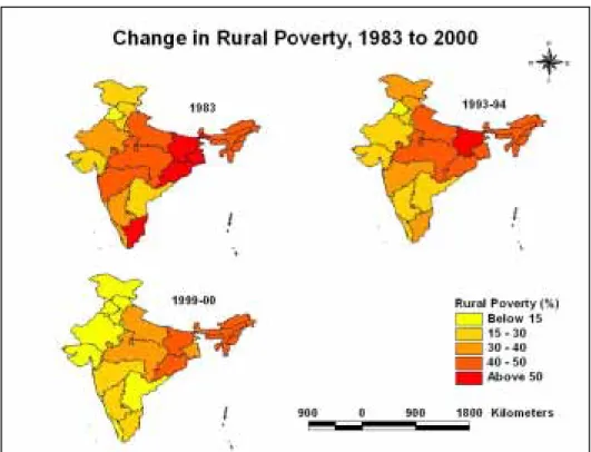
According to the National Human Development Report (GOI 2002) “At National Level the incidence of poverty on the head count ratio declined from 44.48 percent in 1983 to 26.10 percent in 1999-2000. It was a decline of nearly 8.5 percentage points in the ten-year period between 1983 and 1993-94 followed by a further decline of nearly 19 percentage points in the period between 1993-94 and 1999-2000. While the proportion of poor in the rural areas declined from 45.65 percent in 1983 to 27.09 percent in 1999-2000, the decline in urban areas has been from 4.79 percent to 23.62 percent during the period”. Despite achieving a higher economic growth of 6 percent annually during 1990-98, the pace of poverty reduction slowed down in the nineties says the World Development Report 2000-2002. However, the report said that more recently growth has accelerated and poverty has fallen. The report like others highlighted the marked differences in poverty incidence within the country. The report reiterated that poverty reduction would require faster growth which in turn required liberalization especially in agriculture, and better provision of physical and social infrastructure which is lacking in most deprived parts of India.
In spite of the rich data base India has, the debate on accuracy of the figures, use of deflators, reconciling different sets of data available, etc continued to figure in the literature and research for refinements. The official estimate of BPL for India’s population in 1993-94 was placed at 35 percent.
Analysing why some states in India fared better in reducing poverty, (Datt G and Martin Ravallion 1996), showed that there is no sign of trade-offs between growth and pro-poor distributional outcomes. Sound growth in rural areas stemming from State Development spending and presence of good initial physical and human infrastructure was found to be the main factor in poverty reduction as exemplified by Punjab and Haryana. The other approach was based on human resource development as typified by the Kerala experience. The study found that no state had a right mix of both the elements.
Ninan (2000) probed into the role of different factors on poverty levels using time series analysis of all India data and also cross-sectoral data for the two different points of time namely, pre-reform and post-reform period. The study pointed out that policies accelerating agricultural growth, access to PDS, infrastructure development and measures to control inflation helped poverty reduction effectively.
The World Bank (2000) in their report on India summarized “In the mid 1990s growth increased sharply and human development indicators continued to improve. Yet, poverty rates, even in the urban areas, declined only marginally. The inconsistencies between the National Accounts and the National Sample Survey that are used to measure poverty suggest that this may be a statistical artefact”. The report attributes higher average inflation and more rapid increase in food prices in 1990s, and agricultural sector’s inability to raise in labor demand as plausible reasons for this slowdown. It also felt that the disparity in responding to reforms by different states was the fundamental element for the impasse. The report called for among other things an immediate reform in agriculture sector. The report asserts “the issue is not reforms and stabilization, which were clearly needed to correct an unsustainable situation, but incomplete and partial reforms.” Reworking on NSS data and other sources (Deaton & Dreze 2002) a new set of integrated poverty and inequality estimates were presented in a study for India and Indian states for the years 1987-88 and 1999-2000. It endorses the view that poverty declined in the 1990s, yet proceeded more or less on similar line with earlier trends (head-count ratio). However, regional imbalances as reflected by development indicators and growth rates continued during the period. The study found no support for the sweeping claims that the nineties have been a period of ‘unprecedented improvement’ or ‘widespread impoverishment’.
The issue of poverty in the government agenda was on a low priority during 1980s. By the 1990s a new poverty agenda surfaced with the World Bank’s Development Report as a counterpart to the so called “Washington Consensus” on structural reforms (Gita Sen 1999). By this the market-led growth itself was considered as primary and the role of state and focused anti-poverty programs were felt as secondary. Now, the concept of anti-poverty encompasses wider aspects of stakeholder participation, role of governance and livelihood concerns. Levels of income often fail to capture deprivations like – educational deprivation as can be seen in Madhya Pradesh and Andhra Pradesh though the rural poor are less; Kerala, Tamil Nadu and Andhra Pradesh though have lowest levels of child malnutrition, have lowest levels of per capita income. So also, income poverty levels cannot capture richness or poverty of human lives. It is not argued here that income does not count, it matters a lot in improving other factors associated with poverty alleviation. However, the need is to shift attention from income poverty to ‘poverty and inequality of opportunities’ – economic, social and political (Shiv Kumar 2002). Human Development Report and approaches of several aid-giving agencies on livelihoods broadened the concept of poverty beyond a narrow income definition to include dimensions of human deprivations that are critical to quality of life. The definition of poverty thus is multi-dimensional and includes access to social services, self-respect and autonomy. Participation is considered as central to poverty reduction, which encompasses elements of opportunity, empowerment and security (Maxwell et.al 2001).
Figure 1.2.1. Change in rural poverty, 1983-2000.
Figure 1.2.2. Change in urban poverty, 1983-2000.
1.2B. WATER AND LAND RESOURCES OF INDIA
It is well known that the availability and the extent of natural resources of a country – especially land and water – contribute to agricultural growth which is by and large accepted as the “engine of growth” for the economies of several developing countries. India has abundant natural resources, which can be harnessed for a dynamic agricultural growth process in the country.
Covering about 329 million hectares (mha) of area, India comprises different physiographic regions, namely i) the mountainous region of the Himalayas ii) the Indo-Gangetic Plains iii) the central highlands, the peninsular plateau and iv) the eastern and western coastal belts. In addition several islands also come under the territory of the country. India has a land frontier over 15,000 Km and a coastline stretching over 6,000 Km, and is the seventh largest and second most populated country in the world. The mountain ranges of Himalayas, Aravallis, Vindhyas, Sathpuras, Eastern and Western Ghats and the north-eastern ranges are the sources of its streams and rivers, which drain the waters received by rain and snowmelt across the country and joining the Bay of Bengal or the Arabian sea. The Himalayan mountains and the seas around the country influence its climate, which ranges from extreme heat to extreme cold. These climatic conditions in turn influence the distribution of water resources in the country.
i) Water Resources
Nature has bestowed bountiful water resources and sunshine in much of the landmass, which is flat and cultivable in the vast tracts of the Indo-Gangetic plains and costal areas. The land available for cultivation is estimated at 186 mha. There are 24 major rivers flowing in the country with many tributaries linking them. The river basins represent the key source of fresh water – both surface and ground water in the country. The mean annual total discharge of the rivers flowing in various parts of the country is estimated at 1879.45 Km3 (GOI 1995).
The contribution of snow and glacier melt from the Himalayas support the flows in the three main river systems of Indus, Ganges and Brahmaputra, making average yield per unit area double than that of the peninsular river systems, which are dependent on rainfall. More than 50 percent of the water resources of India are located in various tributaries of these three northern rivers. Most of the rivers in the south peninsular India like the Cauvery, the Narmada and the Mahanadi are fed through ground water discharges and are supplemented by monsoon rains thus having limited flows in non-monsoon months (Lal 2001). The long-term average rainfall figures of 117 cm in India are quite high, though they may vary in time and space (100 mm to 11,000 mm). The southwest monsoon during June to September and the northeast monsoon during November to December bring forth rains to the country often accompanied by floods and cyclone disasters.
Considering the rainfall, water availability and agro economic conditions, the Planning Commission’s approach paper to the Ninth Five-Year Plan suggested the following classification of regions in the country (Government of India 1999):
High productivity region: Well developed with irrigation facilities and moderate rainfall like the north-western region of Punjab, Harayana and western Uttar Pradesh or very high assured rainfall like the coastal plains.
Water abundant low productivity region: Areas of low irrigation development and low productivity of agriculture, that have high rainfall and abundant surface and ground water (middle and lower Gangetic Plains, eastern Madhya Pradesh and north-eastern region).
Water scarce low productivity region: Areas with moderate agricultural productivity and low surface and ground water availability (the peninsular India and eastern Rajasthan and Gujarat).
Ecologically fragile regions: The Himalayan slopes and desert areas of Rajasthan.
Except the Ganga – Brahmaputra – Meghna systems, which contribute to more than 60 percent of India’s water resources, several of the small rivers dry up during summer months. Depleting forest cover, heavy silt concentration in rivers and reservoirs cause high flood peaks. Nearly 40 million hectares are flood prone, though not all vulnerable areas are flooded every year. On the other hand about one-third of the country is affected by recurring droughts, earlier 150 districts had been identified as drought prone. As many as 71 districts in 9 states continue to suffer severe drought even after considerable irrigation development… drought has also aggravated regional imbalances in economic development (Government of India 1999).
The National Commission on Integrated Water Resources Development Plan (NCIWRDP) worked out the basin-wise catchment area, its geographical coverage in different states and also the availability of water resources, basin-wise. However, the NCIWRDP recognised the limitations in arriving at 1,953 km3/per year as the country water resource availability. In view of different estimates made by different commissions and committees from time to time and the disparities observed in the statistics, NCIWRDP suggested that the CWC should take up further refinement of the method of assessment of water resources and collection of ‘reliable’ data pertaining to flows and utilization (GOI 1999). The following table 1.2.2 shows the extent of catchment areas of different river basins and the corresponding water resource estimations.
Table 1.2.2: River basins in India: catchment area, coverage and water availability.
Water resource,(km3/per year) River Basin Catchment
area, km2
States covered in the basin
As per CWC 1993
As per NCIWRDP 1999
1 2 3 4 5
Indus 321,289 J&K, Punjab, Himachal Pradesh, Rajasthan and Chandigarh
73.31 73.31 Ganga-Brahmaputra-Meghna
Basin:
Ganga Sub-basin 862,769 Uttar Pradesh, Himachal Pradesh, Haryana, Rajasthan, Madhya Pradesh, Bihar, West Bengal and Delhi UT
525.02 525.02
Brahmaputra sub-basin 197,316 Arunachal, Assam, Meghalaya, Nagaland, Sikkim and West Bengal
#537.24 *629.05 Meghna (Barak) sub-basin 41,157 Assam, Meghalaya, Nagaland, Manipur,
Mizoram and Tripura
48.36 48.36 Subernarekha 29,196 Bihar, West Bengal and Orissa 12.37 12.37
Brahmani-Baitarani 51,822 M.P., Bihar and Orissa 28.48 28.48 Mahanadi 141,589 M.P., Maharashtra, Bihar and Orissa 66.88 66.88 Godavari 312,812 Maharashtra, A.P., M.P., Orissa and
Pondicherry
110.54 110.54 Krishna 258,948 Maharashtra, A.P. and Karnataka ##78.12 **69.81
Pennar 55,213 A.P and Karnataka 6.32 6.32 Cauvery 87,900 Tamilnadu, Karnataka, Kerala and
Pondicherry
21.36 21.36 Tapi 65,145 M.P., Maharashtra and Gujarat 14.88 14.88
Narmada 98,796 M.P., Maharashtra and Gujarat 45.64 45.64 Mahi 34,842 Rajasthan, Gujarat and M.P. 11.02 11.02 Sabarmati 21,674 Rajasthan and Gujarat 3.81 3.81 West flowing rivers of Kutch,
Saurashtra & Luni
334,390 Rajasthan, Gujarat and Daman and Diu 15.1 15.1 West flowing rivers south of
Tapi
113,057 Karnataka, Kerala, Goa, Tamilnadu, Maharashtra, Gujarat, Daman and Diu and Nagar Haveli
200.94 200.94
East flowing rivers between Mahanadi and Godavari
49,570 A.P. and Orissa 17.08 17.08 East flowing rivers between
Godavari and Krishna
12,289 Andhra Pradesh 1.81 1.81 East flowing rivers between
Krishna and Pennar
24,649 Andhra Pradesh 3.63 3.63 East flowing rivers between
Pennar and Cauvery
64,751 A.P., Karnataka and Tamilnadu 9.98 9.98 East flowing rivers south of
Cauvery
35,026 Tamilnadu and Pondicherry UT. 6.48 6.48 Area of North Ladakh not
draining into Indus
28,478 Jammu and Kashmir 0 0 Rivers draining into Bangladesh 10,031 Mizoram and Tripura 8.57 8.57 Rivers draining into Myanmar 26,271 Manipur, Mizoram and Nagaland 22.43 22.43 Drainage areas of Andaman,
Nicobar and Lakshadweep Islands
8,280 Andaman, Nicobar and Lakshadweep 0 0
# Average flow up to Jogighopa as estimated by Brahmaputra Board.
* Includes additional contribution of 91.81 km3 being flow of 9 tributaries joining Brahmaputra downsteam of Jogighopa site. # # Estimate of CWC based on run-off data at Vijaywada site.
** Based on mean flow of the yield series accepted by KWDT Award.
India’s ground water resources are also vast and dispersed. The ground water resources complement the surface storages acting as regulating mechanisms for storing water in the wet season. It has been estimated by the NCIWRDP that as against annual availability of 1,953 km3 (inclusive of 432 km3/year of ground water), approximately 690 km3 of surface water and 396 km3 from ground water resources, totalling 1,086 km3 can be utilized. The estimates of the commission are on a higher side compared to those in other studies. Lal (2001) writes that India “will reach a state of water stress before 2025 when its availability falls below 1000 3 /yr”. According to Lal, the per capita availability of about 2,000 m3 i.e., 2x10³ liters of water per person per year currently estimated would drop down to 1,480 m3 in the ensuing decade.
ii) Soils and Crops
The net cultivated area in the country varies from 180 to 200 mha in different years. The latest available land use pattern figures (GOI 1998) for the year 1994-95 show that 68.39 mha and 11.24 mha of land out of the total reporting area of 284.32 mha was covered under forests and permanent pastures, respectively. The gross cropped area had increased from 131.89 mha in 1950-51 to 188.15 mha in 1994-95. The cropping intensity, which was at 111.07 mha in 1950-51 increased to 131.70 mha, with gross irrigated areas of 22.56 mha and 70.64 mha for the respective years. It is to be noted here that the increase in the gross cropped area was mainly on account of expansion of irrigation. The net irrigated area, however, was 53 mha in 1994-95.
The soils in India are classified into eight groups and their distribution among the six important groups is as follows:
Table 1.2.3. Distribution of soils.
Soils Area (mha) States Features
Alluvial 142.5 Northern areas extending from Rajasthan to West Bengal.
Generally suitable for irrigation. Black 60.3 Madhya Pradesh, Maharashtra,
Karnataka, Andhra Pradesh, Tamilnadu and Orissa. Also found in West Bengal, Bihar, Uttar Pradesh and Rajasthan.
Have high water retaining capacity. Some of them tend to become alkaline and saline after introduction of irrigation. Red 49.8 Tamilnadu, Karnataka, Andhra
Pradesh, Madhya Pradesh, Bihar, Orissa.
Low in moisture, retaining capacity and good permeability. React well to irrigation.
Desert 14.6 Western Rajasthan Sandy and poor in fertility. Laterites 12.1 In heavy rainfall areas of Kerala,
Madhya Pradesh, Andhra Pradesh, Assam, Bihar and Orissa.
Have relatively low organic matter content, low primary minerals and an accumulation of sesquioxides.
Forest Soils 28.1 Madhya Pradesh, Andhra Pradesh, Bihar, Maharashtra .
Deposition of organic matter.
The dominant food crop grown in India is rice. It is grown in areas below sea level to altitudes above 1,979 m. It is cultivated in irrigated as well as in rainfed irrigated conditions and also in shallow or deep water. Rice is grown mostly in Kharif and Rabi seasons. Higher yields are reported generally in the rabi season than in the kharif. An area of 22.84 percent of the gross cropped area was covered under rice during 1994-95. The second important food crop grown is Wheat. The cool winters and warm summers are conducive for a good wheat crop production.