Developing Embedded Control System Platform using Atmel AVR32 Processor: Using Rapid Prototyping with Matlab Real-Time Workshop

(1)

June 2007

Amund Skavhaug, ITK

Master of Science in Engineering Cybernetics

Submission date:

Supervisor:

Norwegian University of Science and Technology

Department of Engineering Cybernetics

Developing Embedded Control System

Platform using Atmel AVR32 Processor

Using Rapid Prototyping with Matlab Real-Time Workshop

(2)

(3)

Problem Description

The goal of this master thesis is to use the new AVR32 processor architecture together with a developed I/O-card in a control system. The control system should be able use Matlab Real-Time Workshop generated code for rapid prototyping.

The assignment consists of:

- Learn how the AVR32 architecture and the STK1000 card works.

- Install developing- and debugging tools for the AVR32 architecture on a Linux workstation. - Make a basic Linux system for the STK1000 card.

- Implement timers for controlling the periodic Matlab execution, and test how accurate these are. - Design and implement a I/O-card using an 8-bit AVR microcontroller.

- Design the interface between the I/O-card and AVR32, and implement a driver the AVR32 can use to control the I/O-card.

- Find out how to compile and run Matlab Real-Time Workshop generated code under Linux on the AVR32 architecture.

- Make Matlab Simulink blocks for the I/O-card.

- Make it easy to use Matlab Real-Time Workshop code on AVR32 for rapid prototyping. - Test and identify the efficiency and limits of the system.

- Make a control system platform with AVR32, that users can build their control system on.

- Make a user manual for the platform that contain the information a user needs to use it, so it can be used with minimal effort.

Assignment given: 08. January 2007 Supervisor: Amund Skavhaug, ITK

(4)

(5)

Preface

This thesis has been very interesting, and a worthy end of my time at NTNU. It has been a privilege to work with a new processor architecture, and try to do something that nobody as far as I know have tried before. I would like to thank Amund Skavhaug, my supervisor, and Haavard Skinnemoen from Atmel Norway. Both of them have been helpful whenever I have needed some guidance.

(6)

(7)

Abstract

AVR32 is a new processor architecture made by Atmel Norway, and in this thesis it has been used to make a control system platform. The hardware used in this platform is the STK1000, an AVR32 development board and an I/O-card. The I/O-card were developed as a part of the thesis. Software for the platform consists of I/O-card firmware, Linux device driver for the I/O-card and user mode drivers.

The platform supports usage of Matlab Real-Time Workshop as a rapid prototyping tool, that generates code from graphical visualization of mathematical models. S-functions were created so Matlab Real-Time Workshop can control the I/O-card.

The control system platform is documented in an user manual. This manual describes how to install development tools for the platform on a Linux or Windows computer, and how to use the it.

(8)

(9)

C Code 117 C.1 ATmega128 . . . 117 C.1.1 Makefile . . . 117 C.1.2 am128main.c . . . 117 C.1.3 am128io.c . . . 118 C.1.4 am128spiSlave.c . . . 122 C.1.5 am128adc.c . . . 122 C.1.6 am128pwm.c . . . 124 C.1.7 am128uart.c . . . 126 C.2 Kernel module . . . 128 C.2.1 Makefile . . . 128 C.2.2 avr32ioc . . . 128 C.2.3 avr32io Cmd.c . . . 131 C.2.4 avr32io SPI.c . . . 135 C.3 User Mode . . . 136 C.3.1 avr32io driver.c . . . 136 C.3.2 avr32io threads.c . . . 139 C.3.3 periodictask.h . . . 141 C.3.4 periodictask.c . . . 142 C.3.5 stopwatch.h . . . 143 C.3.6 stopwatch.c . . . 144 C.4 Matlab S-functions . . . 144 C.4.1 Analog input TLC . . . 144 C.4.2 Analog output TLC . . . 145 C.4.3 Digital input TLC . . . 145 C.4.4 Digital output TLC . . . 146 v

(14)

(15)

Chapter 1

Introduction

Today, computer electronics are found almost everywhere. Many ordinary items contain small embedded computers and new cars have computer controlled breaks, fuel injection and stability control. A computer system that controls a physical system is called a control system, and control systems are continuously getting more complex and smaller in physical size.

In 2006, Atmel Norway released a new processor architecture called AVR32. This processor architecture is designed for use in embedded systems, specially small system with low power consumption. Small physical size and low power consumption are very important for many control systems, specially if the system is battery powered.

The main goal of this thesis was to make use of this new architecture to make a platform for control systems. This will use an AVR32 version of Linux as an operating system, since Linux is an operating system that is free, open source and suited for embedded development. Atmel Norway has ported the Linux kernel and many tools to the AVR32 architecture, so it’s a natural choice.

A control system has to be able to observe and control the environment. To give the AVR32 this capability, an Input/Output-card has been developed. This card makes the AVR32 able to send and receive analog voltage signal from sensors and actuators, and are the AVR32s extension into the physical world.

To make development of control systems easier on the platform, Matlab Real-Time Work-shop was adapted so it can be used as a rapid prototyping tool. This means that code can be generated from Matlab Simulink models, and it runs on the control system. This makes it easy to implement different control systems through the graphical interface of Simulink. The I/O-card can be used in Real-Time Workshop by using the developed Simulink S-function blocks.

To make it easier to use the control system platform, an user manual was written. This contain information about how to install the needed tools and use the control system platform from a Linux distribution or Windows. This is an important part of the thesis, since one of the goals were to make an user-friendly product. The manual should give enough information to use the control system platform. To develop the system further, this report should be read.

(16)

The chapters in this report are as follows:

◦ Chapter 2 Background

This chapter describes some of the technologies and concepts behind the thesis.

◦ Chapter 3 AVR32 Linux on STK1000

This chapter Describes how to install and use AVR32 Linux on STK1000.

◦ Chapter 4 Preliminary tests of AVR32

This chapter performs tests to find out the capabilities of the STK1000 development board and the AVR32 processor architecture.

◦ Chapter 5 Preliminary tests of I/O-card

This chapter performs tests to find out if correct solutions have been chosen for the I/O-card.

◦ Chapter 6 Prototype I/O-card

This chapter describes the design and production of the prototype I/O-card.

◦ Chapter 7 Design of I/O-card software

This chapter describes the design of the I/O-card drivers and firmware.

◦ Chapter 8 Implementation of I/O-card software

This chapter describes the implementation of the I/O-card drivers and firmware.

◦ Chapter 9 Testing with prototype card

This chapter testing the prototype card with the I/O-card drivers and firmware.

◦ Chapter 10 Final version of I/O-card

This chapter describes the design and production of the final version of the I/O-card.

◦ Chapter 11 Matlab Real-Time Workshop

This chapter adapts Matlab Real-Time Workshop to be used as a rapid prototyping tool for the control system platform.

◦ Chapter 12 User manual

This chapter describes how to install the necessary tools and use the control system platform.

(17)

Chapter 2

Background

2.1 Embedded Control System

An embedded control system[14], or control system for short, is a computer system whose main task is to control a physical device or a system. These can vary in sizes, from large and complex systems like a ship or a factory, to smaller devices like a toy robot. A control system will have a predefined task, that won’t change over time. This allows a control system to be more specialized than a workstation computer.

2.1.1 Real-time Constraints

Control systems often have real-time[18] constraints, which means that an operation has to be done both correctly and within a time limit. Hard real-time constraints means that the system will fail with possible disastrous result if a time limit isn’t met. A soft real-time constraint is less serious, and will only lower the quality of the result if failing to meet a time limit.

2.1.2 Input/Output

A control system is useless unless it can measure and manipulate its environment, and to do this the system needs to use sensors and actuators. These instruments may have analog or digital interfaces. If they have analog interfaces, which is quite common, they are controlled with analog input and output (I/O). If the instruments are digital, they probably use a digital communication protocol, like RS-232 or USB.

To be able to use instruments with analog interfaces, a computer needs an I/O-card. These cards have a number of analog I/O channels that can be used with instruments with an analog interface. This normally implies that the card can measure the voltage of a signal (analog input) or make a signal with a given voltage (analog output). I/O-cards often have digital I/O as well, that can be used instead of analog I/O when only digital values (low or high) are used. This is often used together with an analog value, one example is control signals for electrical motor. An analog signal determine the speed or torque of the motor, while a digital signal determines its direction.

(18)

2.2 Atmel AVR32 Architecture

The new AVR32 microprocessor architecture from Atmel Norway claims to be an

architec-ture for the 21st century[2]. Most other processors increase their throughput1by increasing

the clock frequency. The AVR32 microprocessor aims to give high throughput with a slow clock. Since power consumption is directly related to clock frequency, this means that it can do the same work with less power. This will be an important characteristic in the future, since we will use more and more gadgets that use battery as a power source, like hand-held music- and video-players.

Low power consumption is also important for control systems. Many systems needs to have low weight, low cost and a long battery time. Since batteries normally are heavy and expensive, both weight and cost will decrease if the power consumption decrease.

2.2.1 STK1000

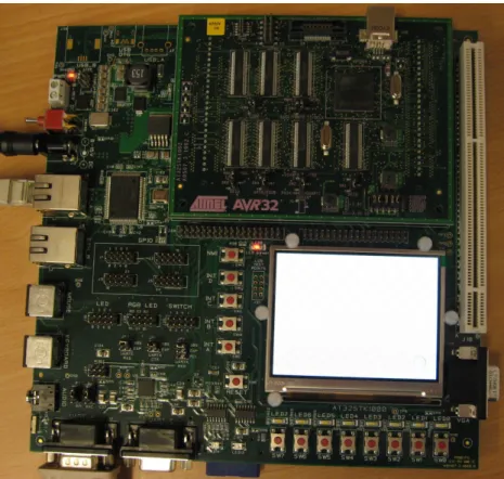
STK1000[8] is a development board for AVR32. STK1000 has some standard I/O connec-tions, like Ethernet, RS-232, mouse and keyboard PS/2. It has an inboard LCD screen and general extension headers where it is possible to connect add-on cards. The STK1000 card comes with a SD flash card with a fully functional Linux system. This is described in more details in 2.3.4. Figure 2.1 on the facing page is an image of the STK1000 board.

2.2.2 AT32AP7000

The AT32AP7000 was the first microprocessor with the AVR32 architecture, and it’s also mounted on the STK1002 daughter-board. that can be connected to the STK1000 board. The features of this processor are listed below.

◦ 32 KB on-chip SRAM.

◦ 16 KB instruction and 16 KB data caches.

◦ MMU and DMA controller

◦ Peripherals like audio DAC, LCD controller, USB 2.0 and two Ethernet MACs.

◦ Serial interfaces like RS-232/USART, TWI (I2C), SPI PS/2.

2.3 Linux

The Linux kernel[15] is an open-source and free2 Unix-like operating system kernel. The

kernel is a single binary program that controls the hardware resources of the computer and makes them available for other running programs. Most people think about Linux, they think about a Linux distribution. However, a distribution is actually a collection of

1

Throughput is a measurement of how much work the processor is able to do.

2

”Free software is a matter of liberty, not price. To understand the concept, you should think offree

as infree speech, not as infree beer.” is a good explanations on free software given inThe Free Software Definition[23]

(19)

2.3. LINUX 5

Figure 2.1: STK1000 development board

programs, including the Linux kernel, that can easily be installed on a computer. They may consist of thousands of programs, but it’s only the kernel that is called Linux.

2.3.1 Linux Control Systems

Linux based operating systems are used in many different systems, from servers and work-stations to embedded systems like control systems. In recent years they have been used more and more in embedded systems. This will most likely increase further in the future,

as indicated in the article in Datarespons’ magazine Interrupt[22]. Below is a list over

reasons to use Linux in a control system, some of these are also mentioned in the article.

◦ Linux and many of the programs running on Linux are free and open-source.

◦ A Linux system is configurable, scalable and able to run on many different hardware

platforms.

◦ Linux is a stable and well tested operating system kernel.

(20)

2.3.2 Kernel Mode and User Mode

Most processor architectures has the ability to run code in different levels of privilege. The

x86 architecture has four, called ring 0 to ring 3. The AVR32 architecture[11] has two

normal modes, calledSupervisor andApplication (equivalent to ring 0 and ring 3). Other

modes are reserved for interrupts and exceptions.

As described on page 19 of Understanding Linux kernel[20], Linux systems uses two of

these levels,kernel mode and user mode. Kernel mode are often refereed to asring 0[19]

and is the highest privileged mode. A normal program executes in user mode but is able

to switch tokernel mode when requesting a service that the kernel provides. Kernel mode

is only used when necessary, and only when allowed by the kernel.

User mode programs can switch to kernel mode or communicate with the kernel through

different interfaces. Asystem call are functions running inkernel mode that can be called

from user mode, and they are described in chapter 10 of [20]. Signals are used to send

notifications betweenuser mode programs, or between the kernel anduser mode programs,

and are described in chapter 11 of [20]. The kernel works as a layer between hardware

devices anduser mode programs, and this is usually done withDevice Drivers. Which are

described in 2.3.3.

2.3.3 Linux Device Driver

A device driver is code that controls a device, normally this is some kind of hardware.

How device drivers works are described in Linux Device Driver[21] and in chapter 13 of

Understanding the Linux kernel[20]. Adevice driver has to be either a part of the kernel or a kernel module that can be linked into a running kernel. Devices are identified in the

Linux kernel with amajor and aminor number. These are numbers that the device driver

has allocated for the devices it controls.

Device drivers are often used to make it possible for user mode programs to use the devices

controlled by the driver. A user mode program access the driver through special files in

the file system, called device nodes. These are normally located in the /dev directory. A

user mode program can read, write or do other file operations on a node, just as if it was a normal file. When accessing a node with the same major and minor number as a device, the user-space program is actually accessing the driver of this device.

There are two types of device nodes, which corresponds to two different types of devices. Character or char devices are devices that receive or send data serially, while block devices receive or send big chunks of data at the time. Most devices except hard drives and RAM are char devices.

2.3.4 AVR32 Linux

AVR32 Linux[3] is a porting3 of the Linux kernel done by Atmel Norway. This means

that it’s a version of the Linux kernel that are able to run on this processor architecture. 3_{Porting software is to do modifications so the software can run on other processors or operating systems,}

(21)

2.4. RAPID PROTOTYPING 7

AVR32 support was included in the mainstream Linux kernel 2.6.19 release, but it doesn’t contain all the drivers for AVR32 and STK1000 board. To get these, it’s necessary to use the AVR32 Linux kernel patches from the AVR32 Linux web page (http://avr32linux.org). Basic system utilities and development tools for the AVR32 architecture can also be found on this web page.

The STK1000 board comes with a SD flash card with a runnable Linux system. This

system includes a patched 2.6.16 version of the Linux kernel andBusybox4. STK1000 uses

U-Boot5, which will boot from the SD card by default. By changing the boot arguments in U-Boot, it is also possible to boot from network. The advantage of network booting is that the kernel image, file system and programs that all have been developed on a workstation can be used by AVR32 Linux through the network. This makes development much faster since new files and programs don’t have to be transferred to a physical medium like a SD card.

To communicate with the AVR32 Linux from a workstation, it’s possible to use both a serial connection and telnet via Ethernet. Both of these solutions are available on the preinstalled Linux system on the SD flash card. They both give a text-based terminal just like a normal text-based Linux system would give. The AVR32 Linux system also has a small web server, that in an embedded control system can be used to display a simple web page with status information and measurement logging.

2.3.5 AVR32 Linux development tools

Atmel Norway has also ported development tools for use with the AVR32 Linux platform. These tools are available precompiled for different Linux distributions and for Windows, or they could be compiled from source. The development tools for AVR32 Linux includes the tools below.

◦ Binutils - GNU Binary utilities for handling object code.

◦ GCC - GNU compiler.

◦ uClibc - A lightweight version of the standard C-library.

◦ u-boot - A boot loader for many different processor architectures.

◦ GDB - GNU debugger that together with a GDB-server on AVR32 can debug code

running on AVR32.

◦ GDB-server - A server version of GDB that can run on the AVR32.

2.4 Rapid Prototyping

In computer engineering, rapid prototyping is a development technique that rapidly make a simplified version of a system. This prototype usually implements a part of the complete

4

Busybox is a lightweight program that includes the functionality of most small Linux applications that an embedded system will need in a single binary file.

5_{U-Boot (Universal bootloader) is a bootloader that can be used on many different platforms, among}

(22)

system, that are necessary to test thoroughly. These are often important parts of the system, and the result of the tests can be used to avoid premature decisions. A typical application is to design the user-interface with a rapid prototyping tool. This allows fast and cheap development of a prototype that the users of the system can test and evaluate. User evaluation can often give important information that is difficult to obtain by other means.

2.4.1 Rapid Prototyping Control Systems

For control systems, rapid prototyping tools can be used to generate control algorithms from graphical visualization of mathematical systems. It’s easier and faster to develop a control system with a tool like this than to write code. It’s also easier to change and search for errors. These generated algorithms can be tested both against simulated and actual systems, which is useful during development. Parts of the algorithms can also be used in the complete system.

Two well known tools for simulating and prototyping of control systems are Matlab and

Labview. Matlab was originally a program for matrix computation (the name stands for MATrix LABoratory), but it has evolved into a large collection of mathematical software. Simulink is one of the programs in this collection, and it’s a program for simulating dynamical system represented by graphical block diagrams. Code can be generated from these block diagrams, making it ideal for rapid prototyping.

Labview uses a data flow language that describes how data flows between different nodes

of a system, often a control system. This language is called G and are the basis of

Labview. The nodes are representations of physical or logical components and can be

placed and connected using a graphical interface. TheGlanguage is a parallel and platform

independent6 _{language and is well suited for prototyping.}

6

(23)

Chapter 3

AVR32 Linux on STK1000

This chapter describes how to install development tools for AVR32 Linux, and how to configure it for development. Some of the problems encountered while working with this version of Linux are described as well.

3.1 Development Tools

Installing the development tools are very easy when using the Ubuntu[10] Linux distri-bution that was used during this thesis. This distridistri-bution uses the Apt[17] (Advanced Packaging Tool) package management tool, that can install software from servers defined

in the/etc/apt/sources.listfile. To add the server containing the AVR32 development

tools, the following line should be added to this file.

deb h t t p : / /www. a t m e l . no / b e t a w a r e / a v r 3 2 / ubuntu / d a p p e r b i n a r y /

To install the tools, execute the following commands, and answer yes to all questions.

sudo a p t i t u d e u p d a t e

sudo a p t i t u d e i n s t a l l a vr3 2−l i n u x−d e v e l

If this approach doesn’t work, or instructions for installing on other platforms, check the

AVR freaks wiki http://www.avrfreaks.net/wiki.

3.1.1 Compiling Development Tools from Source

It’s also possible to compile the development tools from source, and this was necessary during the start of this thesis. Then, the precompiled tools had a few bugs. Compiling the development tools from source is still the only option if special features is needed.

Instructions for doing this can be found at http://avr32linux.org/twiki/bin/view/

Main/GettingStarted.

(24)

3.2 AVR32 Linux Kernel Versions

Some of the early AVR32 versions of the Linux kernel had some problems. Both the 2.6.16, 2.6.18 and 2.6.19 versions were tested. During these tests the following problems was encountered.

◦ The 2.6.16 version had problems linking with the pthread library. The SPI driver

worked, but had problems with stability and returned wrong data.

◦ The SPI driver did not work in the 2.6.18 version.

◦ The 2.6.19 version also had problems linking with the pthread library.

It’s also possible that the problems with the pthread library were because of uClibc, the library used by AVR32 Linux. After switching to the 2.6.20 kernel version and new precompiled development tools, no kernel or library related problems were encountered.

3.3 Configure booting over Network

2.3.4 explains that the STK1000 can be configured to boot over network, and that this is a suitable solution during development.

3.3.1 Workstation Configuration

To boot the STK1000 over network, it’s required that the workstation has two different servers. A TFTP-server (Trivial File Transfer Protocol) are a simple protocol for transfer-ring small files and are used by the boot loader on STK1000 to download the kernel image. A NFS-server (Network File System) are a standard UNIX server for sharing files, and will be used to share a root filesystem with the STK1000 board. For a Ubuntu workstation

these two servers are installed by using aptitude, and the following commands.

˜ $ sudo a p t i t u d e i n s t a l l t f t p d x i n e t d n f s−k e r n e l−s e r v e r portmap

The TFTP-server are configured by adding the following text into /etc/xinetd.conf.

s e r v i c e t f t p { p r o t o c o l = udp p o r t = 69 dgram = dgram w a i t = y e s u s e r = nobody s e r v e r = / u s r / s b i n / i n . t f t p d s e r v e r a r g s = / t f t p b o o t d i s a b l e = no }

The following commands are used to start the server. This is only necessary to do once, afterwards the server starts by itself.

˜ $ sudo mkdir / t f t p b o o t

˜ $ sudo chmod −R 777 / t f t p b o o t ˜ $ sudo chown −R nobody / t f t p b o o t ˜ $ sudo / e t c / i n i t . d/ x i n e t d s t a r t

(25)

3.3. CONFIGURE BOOTING OVER NETWORK 11

The TFTP-server are now started and shares the directory /tftpboot. If a kernel image

are copied to this directory, the STK1000 are able to download and boot this image. The NFS-server are configured by sharing a directory with NFS. This are done in the

/etc/exportfs file, and below is an example of a line that will share a directory.

/home/ o y v i n d n e / m a s t e r / f s 1 2 9 . 2 4 1 . 1 8 7 . 1 / 2 4 ( rw , n o r o o t s q u a s h , a s y n c )

To restart the NFS-server with new configuration, the following commands are used:

˜ $ sudo / e t c / i n i t . d/ portmap r e s t a r t

˜ $ sudo / e t c / i n i t . d/ n f s−k e r n e l−s e r v e r r e s t a r t ˜ $ sudo e x p o r t f s −a

3.3.2 Configure U-Boot

U-Boot (Universal Bootloader) are the boot loader used on STK1000. To configure it, the STK1000 has to be connected to a workstation with a serial cable. The Workstation

should use a serial terminal program like minicom to connect to the STK1000. During

start up of the STK1000 board, the space bar should be pressed to enter the U-Boot

command line. Here, the bootargsvariable has to be changed, and atftpip variable has

to be created. The following commands modify these variables. If used on other systems, the IP addresses to the host computer and the path to the NFS-server has to be changed.

s e t e n v t f t p i p 1 2 9 . 2 4 1 . 1 8 7 . 2 1 2

s e t e n v b o o t a r g s c o n s o l e=ttyUS0 i p=dhcp r o o t =/dev / n f s n f s r o o t = 1 2 9 . 2 4 1 . 1 8 7 . 2 1 2 : / home/ o y v i n d n e / m a s t e r / f s i n i t =/ s b i n / i n i t fbmem=900k

(26)

(27)

Chapter 4

Preliminary tests of AVR32

This chapter describes some preliminary tests performed on the STK1000 board before continuing the work. It was important to reveal any weaknesses the AVR32 architecture may have, so the control system platform can be designed to avoid them as much as possible. It’s also important to test that planned solutions can be used on AVR32.

4.1 Floating-point and Fixed-point operation Test

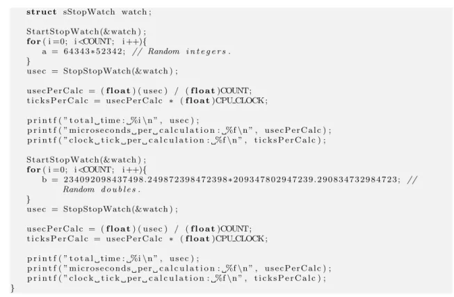
The AVR32 architecture don’t have a hardware floating-point unit (FPU). This means that floating-point operations have to be done with software emulation. Since Matlab RTW generated code normally has many floating-point operations, it’s important to know the processors ability to calculate these. The test referred to in this chapter was set up to reveal this. A test for fixed-point calculations was performed as well, and the two results were compared.

The tests consists of 100 million either floating-point or fixed-point multiplications. The test program measures the time used by these operations, and calculate the number of microseconds and clock cycles one operation takes (on average). To measure the time, the

stopwatch library was used. This library was developed during the thesis, to make time

measurements easier, and consists of stopwatch.h and stopwatch.c that can be found

in the appendix C.3.5 and C.3.6.

4.1.1 Code 1 #include <s t d i o . h> 2 3 #include ” s t o p w a t c h . h ” 4 5 #d e f i ne COUNT 1 0 0 0 0 0 0 0 0

6 #d e f i ne CPU CLOCK 140 // C l o c k f r e q u e n c y o f AVR32 on STK1000 .

7 8 i n t main ( ) 9 { 10 long a ; 11 f l o a t b ; 12 long u s e c , i ; 13 f l o a t u s e c P e r C a l c , t i c k s P e r C a l c ;

(28)

14 s t r u c t sStopWatch watch ; 15 16 S t a r t S t o p Wa t c h (&watch ) ; 17 f o r( i =0; i<COUNT; i ++){ 18 a = 6 4 3 4 3∗5 2 3 4 2 ; // Random i n t e g e r s . 19 } 20 u s e c = StopStopWatch(&watch ) ; 21 22 u s e c P e r C a l c = (f l o a t) ( u s e c ) / (f l o a t)COUNT; 23 t i c k s P e r C a l c = u s e c P e r C a l c ∗ (f l o a t)CPU CLOCK ; 24 25 p r i n t f ( ” t o t a l t i m e : %i\n ” , u s e c ) ; 26 p r i n t f ( ” m i c r o s e c o n d s p e r c a l c u l a t i o n : %f\n ” , u s e c P e r C a l c ) ; 27 p r i n t f ( ” c l o c k t i c k p e r c a l c u l a t i o n : %f\n ” , t i c k s P e r C a l c ) ; 28 29 S t a r t S t o p Wa t c h (&watch ) ; 30 f o r( i =0; i<COUNT; i ++){ 31 b = 2 3 4 0 9 2 0 9 8 4 3 7 4 9 8 . 2 4 9 8 7 2 3 9 8 4 7 2 3 9 8∗2 0 9 3 4 7 8 0 2 9 4 7 2 3 9 . 2 9 0 8 3 4 7 3 2 9 8 4 7 2 3 ; // Random d o u b l e s . 32 } 33 u s e c = StopStopWatch(&watch ) ; 34 35 u s e c P e r C a l c = (f l o a t) ( u s e c ) / (f l o a t)COUNT; 36 t i c k s P e r C a l c = u s e c P e r C a l c ∗ (f l o a t)CPU CLOCK ; 37 38 p r i n t f ( ” t o t a l t i m e : %i\n ” , u s e c ) ; 39 p r i n t f ( ” m i c r o s e c o n d s p e r c a l c u l a t i o n : %f\n ” , u s e c P e r C a l c ) ; 40 p r i n t f ( ” c l o c k t i c k p e r c a l c u l a t i o n : %f\n ” , t i c k s P e r C a l c ) ; 41 } 4.1.2 Result

Table 4.1 shows how the STK1000 preformed on these tests compared to a Dell workstation with a Pentium 4 CPU.

Table 4.1: Results of floating-point (FP) and fixed-point tests

Platform CPU µs/FP cycles/FP µs/fixed cycles/fixed

Dell PC with Ubuntu 2.4GHz 0.00273 6.55 0.00269 6.47

STK1000 140M Hz 0.492 68.8 0.123 17.2

The Pentium is considerable faster than the AVR32, as expected. It uses the same time for both the floating-point and fixed-point operations. This is because it has a floating-point unit. The AVR32 uses about 4 times longer time on a floating-point than on a fixed-point which was regarded as a positive result. It was a bit concerning that the AVR32 uses about 3 times as many clock cycles per fixed-point operation than the Pentium 4, specially since Atmel Norway promise more throughput with lower clock. This may be due to the employed test program inability to compare one fast and one slow processor with each other.

4.2 Timer precision Test

Most control systems have tasks that have to be carried out with regular intervals, every millisecond or shorter. This can be implemented using timers. An easy solution was to use

the internal Linux timers, that has a maximum resolution of 1000Hz. setitimer() will

(29)

4.2. TIMER PRECISION TEST 15

this signal and select a function that runs each time the SIGALRM is received. This is all

done inside a user mode program.

The test consists of 10000 periods of 10ms each. The reason for not choosing 1ms which

is the lowest available timer, is that the standard Ubuntu kernel doesn’t have the highest precision timer (This can be changed by recompiling the kernel, but the test is just as

good with 10ms). The periodic tasks was created using the periodicTask library, that

was developed to make it easy to make and start periodic tasks. This library consists of

periodicTask.h and periodicTask.c, that are in the appendix C.3.3 and C.3.4. The

stopwatch library mentioned in 4.1 was also used.

4.2.1 Code 1 #include <s t d i o . h> 2 #include <math . h> 3 4 #include ” p e r i o d i c t a s k . h ” 5 #include ” s t o p w a t c h . h ” 6 7 #d e f i ne COUNT 1 00 00 8 #d e f i ne PERIODE 1 9 10 i n t main ( ) 11 { 12 i n t i , u s e c [COUNT] , t o t U s e c ; 13 f l o a t t o t V a r , a vrUse c , avrVar , a v r S t d ; 14 s t r u c t s P e r i o d i c T a s k t a s k ; 15 s t r u c t sStopWatch watch ; 16 17 I n i t P e r i o d i c T a s k s ( ) ; 18 S t a r t P e r i o d i c T a s k (& t a s k , PERIODE) ; 19 20 S t a r t S t o p Wa t c h (&watch ) ; 21 22 f o r( i =0; i<COUNT; i ++){ 23 W a i t P e r i o d i c T a s k (& t a s k ) ; 24 u s e c [ i ] = StopStopWatch(&watch ) ; 25 i f( i != COUNT− 1 ) S t a r t S t o p Wa t c h (&watch ) ; 26 } 27 28 t o t U s e c = 0 ; 29 f o r( i =5; i<COUNT−5; i ++){ 30 t o t U s e c = t o t U s e c + u s e c [ i ] ; 31 t o t V a r = t o t V a r + pow ( ( (f l o a t) u s e c [ i ] − 1 0 0 0 0∗PERIODE) , 2 ) ; 32 } 33 a v r U s e c = ( (f l o a t) ( t o t U s e c ) ) / (COUNT−10) ; 34 avrVar = t o t V a r / (COUNT−10) ; 35 a v r S t d = s q r t ( avrVar ) ; 36 37 p r i n t f ( ”Average p e r i o d e t i m e : %f\n ” , a v r U s e c ) ; 38 p r i n t f ( ” V a r i a n c e : %f\n ” , avrVar ) ; 39 p r i n t f ( ”S t a n d a r d d e r i v a t e : %f\n ” , a v r S t d ) ; 40 } 4.2.2 Result

In table 4.2 on the next page the results of the test when performed on different platforms are shown.

STK1000 has the best timer precision of the two machines. The average period is less than the correct value, but the difference is not significant. The standard deviation describes

(30)

Table 4.2: Results of timer tests

Platform CPU Average Standard deviation

Dell Workstation running Ubuntu 7.04 2.4GHz 10013.09µs 2057µs

STK1000 running avr32 Linux 150M Hz 9994.91µs 7.25µs

Sine Wave Scope

1 s Integrator 1

Gain

Figure 4.1: First order low-pass passive filter

how much the results differ from the expected value, and it considerable lower for the STK1000. This is because the workstation computer has many programs running, and these will disturb the timer.

4.3 Test of Matlab Real-Time Workshop Generated Code

One of the goals of this thesis was to configure Matlab RTW to be used as a rapid prototyping tool for the control system. This made it important to check that it was possible to run RTW code on AVR32. A simple test system was created, consisting of a gain block and an integration block, and generated code from it. The GRT system target was used when generating code, see 11.1.1. Figure 4.1 describes the simple test system. To compile the code for AVR32, it was necessary to change the generated makefile. Adding

CC=avr32-linux-gcc to the Makefile (see 11.2.2 for the exact location) specifies that the

AVR32 compiler should be used. When running the Makefile with this addition, the

Makefile returned the following output.

avr3 2−l i n u x−g c c −c −O−f f l o a t−s t o r e −fPIC −m32 −DUSE RTMODEL−a n s i −p e d a n t i c −

DMODEL=t e s t −DRT−DNUMST=2 −DTID01EQ=1−DNCSTATES=1 −DUNIX−DMT=0 −DHAVESTDIO

−I . −I . . −I / u s r / l o c a l / matlab / s i m u l i n k / i n c l u d e −I / u s r / l o c a l / matlab / e x t e r n / i n c l u d e −I / u s r / l o c a l / matlab / rtw / c / s r c −I / u s r / l o c a l / matlab / rtw / c / s r c / ext mode / common −I /home/ o y v i n d n e / d i p l o m / matlab / s i m p l e T e s t / t e s t g r t r t w −I /home/ o y v i n d n e / d i p l o m / matlab / s i m p l e T e s t −I / u s r / l o c a l / matlab / rtw / c / l i b s r c r t n o n f i n i t e . c c c 1 : e r r o r : i n v a l i d o p t i o n ’ 3 2 ’

make : ∗∗∗ [ r t n o n f i n i t e . o ] E r r o r 1

The compilation ends with an error, since the AVR32 compiler doesn’t understand the

-m32 flag. When removing this from the Makefile, the compilation is successful, and the

compiled program runs on the STK1000 card with no problems. Notice that during the first AVR32 compilation in a folder, many object files are compiled, since the default

ones from Matlab are all i386 specific. These files are only compiled once, so future

compilations will take much shorter time.

4.4 Preliminary Test Conclusion

After doing these tests it was concluded that the AVR32 processor can be used in a control system, even if the floating-point performance wasn’t impressive. This weakness implies

(31)

4.4. PRELIMINARY TEST CONCLUSION 17

that use of floating-point has to be minimized whenever possible. In situations where it’s impossible or hard to avoid using floating-point, it can be used, even if it means that the effectiveness of the program is reduced.

The timer test gave a good result, and these timers will be used through the thesis. They

give good precision for timers down to 1ms. The AVR32 will probably be best suited

for control systems with higher periods than 1ms, because of the slow clock and poor

floating-point performance. The last test in this chapter confirmed that the AVR32 can run code generated by Matlab RTW, after a few modifications.

(32)

(33)

Chapter 5

Preliminary tests of I/O-card

2.1.2 describes why control systems need I/O, specially analog I/O. Since the STK1000 don’t have any analog I/O, a I/O-card was developed. This chapther performs test to find out if the chosen ATmega128 microcontroller is able to work as a controller for the I/O-card, and if the SPI-bus is useable as communication between STK1000 and the I/O-card.

5.1 AVR Microcontroller

5.1.1 ATmega128

An ATmega128[1] microcontroller was used to control the I/O-card. This is a 8-bit mi-crocontroller from the AVR family from Atmel Norway. ATmega128 is a 64-pin

micro-controller with 128kB flash and 4096B SRAM, making it one of the AVRs with highest

specification. Some of the features of the ATmega128 are shown below.

◦ 8-channel 10-bit ADC (analog input).

◦ 2-channel 16-bit PWM (Pulse Width Modulator) timers with 3 subchannels each.

These can be used as analog output.

◦ 2 8-bit timers.

◦ 2 USARTs that can be converted RS-232.

◦ Several external interrupts.

◦ SPI (Serial Peripheral Interface).

◦ TWI (Two-Wire Interface).

◦ Several general digital I/O pins (digital I/O).

With these built-in features, there was no need for extra analog I/O components. This microcontroller could do both the communication with the STK1000 board and the actual I/O. This made the design of an I/O card easier.

(34)

5.1.2 STK500/501

The STK500[9] is an AVR development board that is well suited for early stage devel-opment of AVR microcontrollers. To use this board with the ATmega128 model, it’s necessary to use the expansion module STK501, which supports 64 pins surface mounted AVRs. When using STK500/501 all the pins of the used AVR are available as headers, and all the basic components that the AVR often uses like clock source and RS-232 circuit are ready to use.

This development board was used to test how different features of ATmega128 could be used before making a prototype I/O-card. These test helped minimizing the number of design errors on the prototype.

5.2 Analog input

Analog input are used to measure the voltage of signals, and are done with ADCs (Analog-Digital Converter). These are important for a control system, to receive measurement data from sensors. The I/O-card will use the ADC on the ATmega128. This is a 8-channel 10-bit ADC that can measure the voltage between two pins or between a pin and ground.

This ADC can convert voltages betweenGN D and AVCC (analog supply).

5.2.1 Test of ATmega128 ADC

The ADC of ATmega128 was tested by connecting different voltages from STK1000 (2.5V,

3.3V and 5V) to one of the analog in channels. The code below starts an ADC conversion

and shows the result (8 MSB) on the LEDs after it was completed. Table 5.1 on the next page shows the results.

1 // I n c l u d e s . 2 #include <a v r / i o . h> 3 4 // Macros f o r b i t o p e r a t i o n s . 5 #d e f i ne s e t b i t ( r e g , b i t ) ( r e g |= ( 1 << b i t ) ) 6 #d e f i ne c l e a r b i t ( r e g , b i t ) ( r e g &= ˜ ( 1 << b i t ) ) 7 #d e f i ne t e s t b i t ( r e g , b i t ) ( r e g & ( 1 << b i t ) ) 8 9 i n t main ( ) 10 { 11 // D i r e c t i o n o f p o r t s . 12 DDRC = 0 x f f ; 13 c l e a r b i t (DDRF, 0 ) ; 14 15 // I n i t i a l i z e ADC.

16 ADMUX = (1<<REFS0 ) | (1<<ADLAR) ;

17 ADCSRA = (1<<ADEN) | (1<<ADPS2) | (1<<ADPS1) ; 18

19 // S t a r t c o n v e r s i o n .

20 s e t b i t (ADCSRA, ADSC) ; 21

22 // Wait f o r c o n v e r s i o n .

23 while( ! t e s t b i t (ADCSRA, ADIF) ) ; 24

25 // S e t r e s u l t a s o u t p u t t o LEDs .

26 PORTC= ADCH; 27 }

(35)

5.3. ANALOG OUTPUT 21

Table 5.1: Results of ADC test

Voltage Multimeter voltage ADC result (8 bit) ADC result in voltage

2.5V 2.50V 113 2.21V

3.3V 3.27V 136 2.66V

5V 5.00V 210 4.12V

As seen in table 5.1, the results from the ADC were not very accurate. All results were

80%−90% of the correct value. It might be because of an error with the STK500/501

card or maybe the ATmega128.

5.3 Analog Output

Analog output is used to make an analog voltage. This is important for control system, so they are able to control actuators. The I/O-card will use PWM (Pulse-Width Modulation) of the ATmega128 to generate an analog signal. PWM is a digital signal with a constant frequency and a controllable duty-cycle. The duty-cycle is a value that describes how much of the period the digital signal is high. A 50% duty-cycle means that the signal is high half of the periode, then low the rest of the periode, and will look like square-wawe signal.

5.3.1 Generating Analog Signal from PWM

A low-pass filter is also called an “averaging” filter, and it will convert the PWM signal into an analog voltage equal to the average voltage of the PWM-signal. This analog voltage can be set by varying the duty-cycle of the PWM, making this a digital-to-analog conversion (DAC). An example of a PWM-signal before and after a first-order low-pass filter are shown in figure 5.1 on the next page. As all the figures describing PWM signals shows what happens when a PWM duty-cycle increases from 0% to 50%, which is the same as

the DAC increases it’s value from 0V to 2.5V.

5.3.2 Quality of Analog Signal

The quality of an analog signal made with a PWM can be described with two values. The ripple is how much the output varies, and the response-time is how fast the output change when the duty-cycle change. The second-order filter in figure 5.2 on the following page has ripple marked with green. The ripple are measures as the amplitude of the

signal between the green dotted lines, in the figure about 0.15V. The response time are

defined throughout this report as the time used to increase from 0V to 2V when the DAC

increases from 0V to 2.5V. This are marked with red in the figure and is about 300µs.

There are many factors that influence the ripple and response time of the DAC, and these are explained below.

(36)

0 1 2 3 4 5 x 10−4 0 0.5 1 1.5 2 2.5 3 3.5 4 4.5 5 5.5 Time Volt first−order filter PWM

Figure 5.1: PWM signal and PWM signal with first-order low-pass filter.

0 0.2 0.4 0.6 0.8 1 x 10−3 0 0.5 1 1.5 2 2.5 3 3.5 4 4.5 5 Time Volt

(37)

5.3. ANALOG OUTPUT 23

Figure 5.3: First order low-pass passive filter

0 0.2 0.4 0.6 0.8 1 x 10−3 0 0.5 1 1.5 2 2.5 3 3.5 4 4.5 5 Time Volt RC = small RC = large

Figure 5.4: PWM signal filtered with filters with different Time constants (RC)

5.3.3 Time constant (RC)

A simple passive1low-pass filter consists of a resistor and capacitors as shown in figure 5.3.

The time constant (RC) of the filter is the product of the resistance and capacitance of these two components, and it describes how the filter works.

When using a low-pass filter to convert a PWM-signal to an analog signal, the time constant defines the response time of the DAC. A low time constant will give a “fast” filter, while a high time constant will give a “slow” filter. A fast filter will increase the ripple of the analog signal. Figure 5.4 shows how two second-order filters with different time constants (RC) filters the same PWM-signal.

1_{A filter is passive if it only consists of passive components like resistors, capacitors and inductors.}

(38)

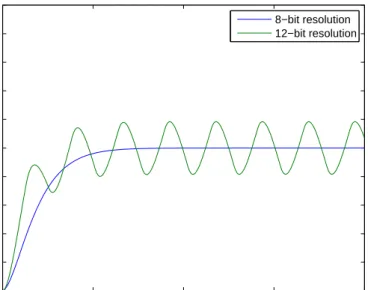
0 0.5 1 1.5 2 x 10−3 0 0.5 1 1.5 2 2.5 3 3.5 4 4.5 5 Time Volt 8−bit resolution 12−bit resolution

Figure 5.5: 8-bit and 12-bit DAC with equal filters.

5.3.4 Frequency and Resolution

The frequency of the PWM-signal depends on the clock frequency of the device (the mi-croprocessor) that makes the PWM and the resolution of the DAC. Equation 5.1 describes how the frequency of the PWM-signal can be calculated.

fP W M =

fclock

2bits (5.1)

A high PWM frequency will give lower ripple than a low PWM frequency. This means that increasing the resolution will increase the ripple. Figure 5.5 shows a 8-bit and a 12-bit resolution DAC filtered with the same filter. It shows that the response time is about the same for both, but the 12-bit resolution result has significant ripple.

5.3.5 Order of low-pass Filter

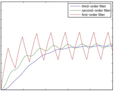
By adding several first-order filters after each other, a higher order filter is created. The second filter will then filter the result of the first filter and so on. Figure 5.6 on the next page shows a DAC with equal (same RC) filters of different orders, and it shows that each filter reduces ripple but increases response time.

5.3.6 Test of ATmega128 PWM as DAC

5.3.1 explains how a PWM-signal can be used to make an analog voltage. This should be possible to do with the ATmega128 since it has several timers that can be used as PWM. Timer 1 and 3 was used for this, since these have changeable resolutions up to 16 bits.

(39)

5.3. ANALOG OUTPUT 25 0 1 2 3 4 5 x 10−4 0 0.5 1 1.5 2 2.5 3 3.5 4 4.5 5 Time Volt third−order filter second−order filter first−order filter

Figure 5.6: DAC with equal (same RC) first, second and third-order filters.

The STK500/501 board was used to test the PWM. This was done by starting PWM on the different outputs, while probing them with an oscilloscope.

The code below starts a 10-bit PWM-signal with 50% duty-cycle to the first output of timer 1. This should give a square-signal with a frequency given by the equation 5.2 on the following page.

1 // I n c l u d e s . 2 #include <a v r / i o . h> 3 4 i n t main ( ) 5 { 6 // S e t t h e t i m e r 1A a s o u t p u t . 7 s e t b i t (DDRB, 5 ) ; 8 9 // S e t t h e c o n t r o l r e g i s t e r s f o r PWM t o f a s t PWM, w i t h no p r e s c a l e r and c l e a r o u t p u t

10 // on compare match ( non−i n v e r t i n g mode ) .

11 TCCR1A =(1<<COM1A1) | (1<<COM1B1) | (1<<COM1C1) | (1<<WGM11) ; 12 TCCR1B = (1<<WGM13) | (1<<WGM12) | (1<<CS10 ) ; 13 14 // S e t r e s o l u t i o n o f PWM t o 1 0 . 15 ICR1H = 0 x03 ; 16 ICR1L = 0xFF ; 17 18 // S e t 50% d u t y c y c l e . 19 OCR1AH = 0 x02 ; 20 OCR1AL = 0 x00 ; 21 }

With a 10-bit PWM-timer and a clock frequency of 8M Hz, the PWM-frequency are

calculated in equation 5.2 on the next page. When running this test, the period of the

PWM signal was measured to 130µson an oscilloscope, that according to equation 5.3 on

(40)

fP W M = 8M Hz 210 = 7.81kHz (5.2) fP W M = 1 130µs= 7.69kHz (5.3)

5.4 SPI

To be able to use the I/O-card, the AVR32 needs a way to communicate with it. SPI is a serial bus that’s often used for communication between different integrated circuits on the same board. It’s an simple yet effective bus that is full duplex, meaning that data are transferred in both directions at the same time. Both AVR32 Linux and the ATmega128 supports SPI, and this bus will be used for data transfer between the STK1000 board and the I/O-card.

Another serial bus called I2C (Inter-Integrated Circuit) or TWI (Two-Wire Interface) was also considered, and was also supported by AVR32 Linux and ATmega128. This bus does about the same as SPI, but the differences described in 5.4.1 made the SPI a better choice.

5.4.1 SPI bus

A SPI bus consists of one master and one or more slaves. The master can communicate with one slave at the time by using the slaves “chip-select” signal. This is different than I2C, that uses addressing to decide which device that should receive the message. By using “chip-select” signals the SPI doesn’t need to start each data package with an address, meaning that a SPI package only contain data, while a I2C package contain an address and data. This makes SPI more effective when only a few devices uses the bus.

When more devices uses the bus, SPI won’t be a good choice. This is because each device needs its own “chip-select” signal, meaning a dedicated pin on the master for each of the slaves. It’s also possible to use an additional component that decodes an address to several slave select signals.

The SPI bus consists of four types of signals describes below. All the devices on the bus also needs common ground.

◦ MOSI (Master Out Slave In) sends data from the master to the slave.

◦ MISO (Master In Slave Out) sends data from the slave to the master.

◦ SCK (Serial ClocK) is the common clock sent by the master. Since it’s a common

clock on the bus, the bus is synchronous.

◦ CS (Chip Select) or SS (Slave Select) is a signal that master send to start a transfer

(41)

5.5. TEST OF SPI COMMUNICATION BETWEEN AVR32 AND ATMEGA128 27

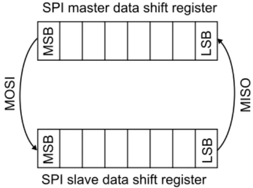
Figure 5.7: How data are transferred between SPI master and slave.

5.4.2 SPI transfer

When using SPI it’s important to know how the data is transferred. Each device on the bus has a SPI data register, and during a transfer between two devices the content of their SPI data registers is exchanged. This is described in figure 5.7. It means that before the transfer both devices need to place what they want to send in their data register, and after the transfer the data in the register is the received data. Since data is sent both ways at the same time, SPI is full duplex.

If the master just wants to send data, not receive, the received data can be dropped. If

the master wants to receive data, a dummy byte2_{has to be sent, since the slave can’t send}

anything when the master doesn’t.

The slave can’t initialize a data transfer, and this may give some problems. Specially if the slave has to complete something, and then report back to the master. This can be solved

by letting the master poll3 the slave until it is finished. This will slow down both the

master and slave. A more effective solution is to let the slave trigger an external interrupt on the master when it’s finished.

5.5 Test of SPI communication between AVR32 and

AT-mega128

By connecting the STK1000 and STK500 boards, it was possible to test SPI communica-tion between the two processors. It was important to find out if SPI would work before designing the I/O-card.

2_{A dummy byte is a byte that contain data of no value, and is just used to request data from the SPI}

slave. The dummy byte can have any value, but should be chosen to a value that the slave won’t believe is something else.

3_{In this context, polling is to periodically ask if something is finished until the answer is yes. This is}

(42)

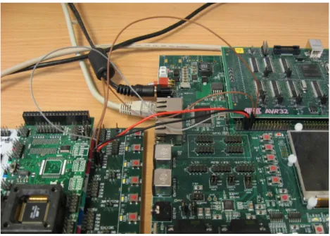
Figure 5.8: Image of STK500 and STK1000 with SPI connection

Figure 5.9: SPI wires between STK500 and STK1000.

5.5.1 Hardware setup

SPI signals are available on headers on both STK cards, and they were connected with short cables, like on the figure 5.8. Figure 5.9 shows which pins on the header that are used. The signals are connected as follows: MOSI, MISO and SCK should be connected to the same signal, while the NPCS2 on STK1000 should be connected to the SS signal on STK500. The two processors must also have common ground to communicate with SPI.

5.5.2 AVR32 as SPI master

As most hardware, the SPI driver can’t be accessed directly from user mode. To make it possible, a device driver has to be made. 8.2 describes how the device driver for the

(43)

5.5. TEST OF SPI COMMUNICATION BETWEEN AVR32 AND ATMEGA128 29

I/O-card was implemented, and the device driver used for this test was similar. During the test the device driver sends the value 222 to the SPI slave, and it prints out the returned value.

5.5.3 ATmega128 as SPI slave

SPI with ATmega128 is used by reading and writing three SPI-specific registers. The control register (SPCR), the status register (SPSR) and the data register (SPDR). How these registers are used in slave mode is described below.

◦ SPCR

• Bit 0 (SPR0) and bit 1 (SPR1) aren’t used in slave mode

• Bit 2 (CPHA) and bit 3 (CPOL) defines the mode. The different

SPI-modes have different timing between the clock signal and the data signals. All devices using the same SPI-bus need to use the same mode.

• Bit 4 (MSTR) selects slave mode when written to zero.

• Bit 5 (DORD) selects if the LSB or MSB should be sent first during transfer.

All devices using the same SPI-bus should use the same data order, or data needs to be reversed in software.

• Bit 6 (SPE) turns on SPI for this device.

• Bit 7 (SPIE) turns on SPI-interrupts for this device.

◦ SPSR

• Bit 0 (SPI2X) isn’t used in slave mode

• Bit 1 to 5 are reserved bits.

• Bit 6 (WCOL) is set if the data register is written to during transfer.

• Bit 7 (SPIF) is set when a SPI-transfer is completed. Will trigger an interrupt

if bit 7 of SPCR is high.

◦ SPDR is used both to send and receive data. The data in the register before transfer

will be sent to the master, while the data in the register after transfer is the data received from the master. Writing or reading to this register clears bit 7 of SPSR. The simple program below was used, to test the SPI communication. It waits for a SPI transfer initialized by a SPI master. The slave will send the value 111 to the master and it will use the LEDs on the STK500 to display the received data. This confirms that the SPI communication works both ways.

1 // I n c l u d e s . 2 #include <a v r / i o . h> 3 4 i n t main ( ) 5 { 6 // I n i t i a l i z e SPI . 7 SPCR = (1<<SPE) ; 8 DDRB = (1<<3) ; 9 10 // I n i t i a l i z e LEDs .

(44)

11 DDRD = 0 x f f ; 12 PORTD = 0 ; 13 14 // S e t d a t a . 15 SPDR = 1 1 1 ; 16 17 // Wait f o r t r a n s f e r .

18 while( ! ( SPSR & (1<<SPIF ) ) ) ; 19

20 // Send r e c e i v e d d a t a t o LEDs and l o o p f o r e v e r .

21 PORTD = SPDR ; 22 while( 1 ) ; 23 }

5.5.4 Result

The test of a simple SPI transfer between the two STK boards was successful. This means that it will be possible to use SPI as communication between AVR32 and an I/O-card. The

highest SPI frequency that worked was measured to about 1.90M Hzwith an oscilloscope.

According to the ATmega128 data sheet[1] both the low and high period of the SCK signal

has to be longer than 2 clock cycles. When the clock frequency is 8M Hz this means that

(45)

Chapter 6

Prototype I/O-card

This chapter desribes the design and production of the first of two I/O-card versions produced during this thesis. The first card is called the prototype card, and was designed to be ideal for testing and debugging.

6.1 PCB Software

A PCB (Printed-Circuit Board) is an epoxy bonded fiberglass sheet with copper layers that can be etched or milled off and leave electrical circuits. Most electronics are implemented on PCBs, and they may have different numbers of layers, and each layer can contain circuits.

There are a number of different software solutions for designing PCBs. In this thesis the freeware version of Eagle[4] was used. This program has a limitation on the size of the finished card, and it can’t design cards with more than two layers. This wasn’t a problem,

since the maximum size (8x10cm) and two layers were enough for the purpose.

6.2 Features

This card was designed to have these features:

◦ ATmega128 with 16 MHz crystal as controller.

◦ JTAG-interface for ATmega128.

◦ Reset button for ATmega128.

◦ RS-232 connection for debugging to a serial port on a workstation.

◦ Header ready to connect to general expansion header on STK1000 with power-supply,

SPI and interrupt signals.

◦ Jumper for choosing between external power-supply and power-supply from STK1000.

◦ 2 AVR32 interrupts that can be triggered from ATmega128.

(46)

◦ 2 AVR32 interrupts that can be triggered externally.

◦ 2 ATmega128 interrupts that can be triggered externally.

◦ 6 channel 8 to 12-bits analog output.

◦ 8 channel 10-bits analog input.

◦ Common ground for both STK1000 and STK500.

◦ 8 channel digital output.

◦ 8 channel digital input.

◦ SPI signals available on ”debug” header.

6.3 Components

The components used for this card:

◦ ATmega128 microcontroller ([1]).

◦ MAX233 UART to RS-232 IC ([5]).

◦ Two 100nF capacitors for decoupling ATmega128 and MAX233).

◦ Linear voltage regulator (7805) with capacitors ([7]).

◦ 100nF capacitor and 10µH inductor for LC filter on analog supply.

◦ 16M Hz crystal and two 18pF capacitors for crystal circuit for ATmega128.

◦ One button, 10kΩ resistor and 100nF capacitor for reset button for ATmega128.

◦ Six second-order RC-filter for filtering PWM signal to analog value. Two resistors

and two capacitors for each filter.

◦ 3 operational amplifiers (MC1458) ([6]).

◦ Screw clamps for connecting different signals.

◦ 2x5 male header for JTAG connection.

◦ 2x18 male header for STK1000 connection.

◦ 1x3 male header with jumper for power-supply selection.

◦ 1x8 header for debug signals.

6.4 Schematic

The schematic of a circuit is a logical representation of how the different parts connects to each other. When designing a circuit, it’s normally best to start with this. The whole schematic are in the appendix B.1. Different sections of the circuit are presented below. Be aware that these are the orignal schematics of the prototype, and have errors described in 6.7.

(47)

6.4. SCHEMATIC 33

Figure 6.1: Power circuit

Figure 6.2: Reset, crystal and analog reference circuits for ATmega128

6.4.1 Power Circuit

Figure 6.1 shows the Power circuit used for the I/O-card. To the left are the power jack connector, for connecting a AC/DC adapter. In the bottom right corner, there is a linear

voltage regulator7805[7] that gives out a stable 5V voltage source. This component needs

a capacitor on both input and output to work properly. On the top there is a 3-pin header. A jumper is used to choose what kind of voltage source the rest of the card will use, either

(48)

Figure 6.3: JTAG header and analog input connectors

6.4.2 Reset, Crystal and Analog Supply Circuit

Figure 6.2 on the previous page shows the reset, crystal and analog reference circuits for the ATmega128. The reset circuit provides a button that will “pull-down” the active-low reset port of the microcontroller when pushed. This will reset the processor. This circuit also has a “pull-up” resistor that makes sure the reset port is high when the button isn’t pushed.

The crystal circuit was made to give the ATmega128 a stable and high frequency clock source. The main reason for this is that a higher clock frequency will make the PWM signal better suited as a base for making analog out signals.

The analog supply is necessary to make the ATmega128 able to read analog input signals. The crystal and analog supply circuits are implemented after specification given in the ATmega128 data sheet [1].

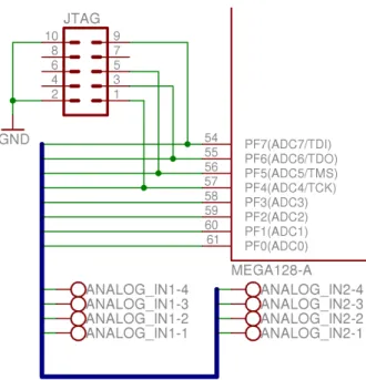
6.4.3 JTAG header and Analog Input Connectors

Figure 6.3 shows the JTAG header for the ATmega128 and screw clamps for the analog input signals. The JTAG header was added to allow a AVR JTAG ICE (either original or mk2) to connect, program and debug the ATmega128. The analog input screw clamps was mounted at the side of the I/O card, and makes it easy to connect wires with analog signals to the ADC of the ATmega128. Four of ATmega128s ports was used both by the JTAG header as analog input. This shouldn’t be a problem as long as no analog signals are connected to these ports when using the JTAG header.

(49)

6.4. SCHEMATIC 35

Figure 6.4: RS-232 circuit and digital output connectors

6.4.4 RS-232 circuit and Digital Output Connectors

Figure 6.4 shows a circuit for RS-232 interface for ATmega128 so it can connect to a serial cable on a PC. The microcontroller has two UART signals, and one of these was converted into a RS-232 signal with the MAX233 ([5]) from Maxim. This signal was made available on a 9-dsub connector, that connects to a normal serial cable.

The figure also shows screw clamps for digital out signals of the I/O-card. Like the analog in, these will be placed on the edge of the card.

6.4.5 STK1000 headers and Digital Input Connectors

Figure 6.5 on the following page shows the circuit for STK1000 headers and digital in signals (same as for digital output). A 36 pin header are used to connect to one of the expansion headers on the STK1000 board. This header includes signals for SPI, interrupts

and ground. The I/O-card can also draw power from the 5V source from STK1000. Two

of the interrupts are connected directly to the ATmega128, and two are available on screw clamps.

To make debugging simpler, a header was placed on the card that had pins for the different SPI signals. These pins makes it easy to probe these signals and look at them on an oscilloscope.

6.4.6 Decoupling Capacitors and VCC/GND Connectors

Figure 6.6 on the next page shows a small but important part of the I/O-card. This is the two capacitors that are used for decoupling the ATmega128 and MAX233. Decoupling is important since it ensures that these ICs gets a stable power supply. The figure also shows

(50)

Figure 6.5: STK1000 headers and digital input connectors

(51)

6.4. SCHEMATIC 37

Figure 6.7: Analog out circuit

two screw clamps that has VCC and GND signals. These signals are available for devices connecting to the I/O card, and are necessary because all I/O signal needs a reference.

6.4.7 Analog Output Circuit

Figure 6.7 shows the filters and operational amplifiers (op-amp) that are used to convert the PWM-signal into an analog voltage. Each of the 6 analog output subchannels has its own second-order passive low-pass filter, that smooth the PWM signal to a constant analog

voltage between 0V and 5V. These filters consists of two resistors and two capacitors

each. The 6 subchannels can have different filters, and since this is a prototype card, it’s imperative that several different filters are tested.

The reason for choosing a second-order filters are that it will give a good compromise between ripple, response and physical size. A first-order filter would give too much ripple, while a higher order filer would take too much physical space. Figure 6.8 on the next page shows that by using different cut-off frequencies it’s possible to get similar behavior from a second and a third order filter. This means that higher order filter not necessarily gives a better result.

After each filter, an op-amp circuit is placed. These are voltage followers, which means that their output voltage is the same as their input voltage. They are not used for amplifying the voltage, but they are used to amplify the current, since an op-amp can supply a lot more current than an ATmega128 can. The op-amps high input impedance, means that the current flowing from the ATmega128, through the filter and to the op-amp are minimal. This is important since the properties of passive filters depends on the current flowing through. High current, will mean a high voltage loss in the resistors of the filter.

Developing Embedded Control System Platform using Atmel AVR32 Processor: Using Rapid Prototyping with Matlab Real-Time Workshop

June 2007

Amund Skavhaug, ITK

Master of Science in Engineering Cybernetics

Submission date:

Supervisor:

Norwegian University of Science and Technology

Department of Engineering Cybernetics

Developing Embedded Control System

Platform using Atmel AVR32 Processor

Using Rapid Prototyping with Matlab Real-Time Workshop

Preface

Abstract

Contents

Chapter 1

Introduction

Chapter 2

Background

2.1

Embedded Control System

2.2

Atmel AVR32 Architecture

2.3

Linux

2.4

Rapid Prototyping

Chapter 3

AVR32 Linux on STK1000

3.1

Development Tools

3.2

AVR32 Linux Kernel Versions

3.3

Configure booting over Network

Chapter 4

Preliminary tests of AVR32

4.1

Floating-point and Fixed-point operation Test

4.2

Timer precision Test

4.3

Test of Matlab Real-Time Workshop Generated Code

4.4

Preliminary Test Conclusion

Chapter 5

Preliminary tests of I/O-card

5.1

AVR Microcontroller

5.2

Analog input

5.3

Analog Output

5.4

SPI

5.5

Test of SPI communication between AVR32 and

AT-mega128

Chapter 6

Prototype I/O-card

6.1

PCB Software

6.2

Features

6.3

Components

6.4

Schematic