Spatio-Temporal Variability of Droughts and Terrestrial Water Storage
1
over Lake Chad Basin using Independent Component Analysis
2
Christopher E. Ndehedehea, Nathan O. Agutua,b, Onuwa Okwuashic, Vagner G. Ferreirad
3
aWestern Australian Centre for Geodesy and The Institute for Geoscience Research Curtin University, Perth,
4
Australia.
5
bDepartment of Geomatic Engineering and Geospatial Information systems JKUAT, Nairobi, Kenya.
6
c
Department of Geoinformatics and Surveying, University of Uyo, P.M.B. 1017, Uyo, Nigeria.
7
d
School of Earth Sciences and Engineering, Hohai University, Nanjing, China
8
Abstract 9
Lake Chad has recently been perceived to be completely desiccated and almost extinct due
10
to insufficient published ground observations. Given the high spatial variability of rainfall in
11
the region, and the fact that extreme climatic conditions (for example, droughts) could be
12
intensifying in the Lake Chad basin (LCB) due to human activities, a spatio-temporal
ap-13
proach to drought analysis becomes essential. This study employed independent component
14
analysis (ICA), a fourth-order cumulant statistics, to decompose standardised precipitation
15
index (SPI), standardised soil moisture index (SSI), and terrestrial water storage (TWS)
de-16
rived from Gravity Recovery and Climate Experiment (GRACE) into spatial and temporal
17
patterns over the LCB. In addition, this study uses satellite altimetry data to estimate
vari-18
ations in the Lake Chad water levels, and further employs relevant climate teleconnection
19
indices (El-Ni˜no Southern Oscillation-ENSO, Atlantic Multi-decadal Oscillation-AMO, and
20
Atlantic Meridional Mode-AMM) to examine their links to the observed drought temporal
21
patterns over the basin. From the spatio-temporal drought analysis, temporal evolutions of
22
SPI at 12 month aggregation show relatively wet conditions in the last two decades (although
23
with marked alterations) with the 2012−2014 period being the wettest. In addition to the
24
improved rainfall conditions during this period, there was a statistically significant increase of
25
0.04 m/yr in altimetry water levels observed over Lake Chad between 2008 and 2014, which
26
confirms a shift in the hydrological conditions of the basin. Observed trend in TWS changes
27
during the 2002−2014 period shows a statistically insignificant increase of 3.0 mm/yr at the
28
center of the basin, coinciding with soil moisture deficit indicated by the temporal evolutions
29
of SSI at all monthly accumulations during the 2002−2003 and 2009−2012 periods. Further,
30
SPI at 3 and 6 month scales indicated fluctuating drought conditions at the extreme south of
31
the basin, coinciding with a statistically insignificant decline in TWS of about 4.5 mm/yr at
the southern catchment of the basin. Finally, correlation analyses indicate that ENSO, AMO,
33
and AMM are associated with extreme rainfall conditions in the basin, with AMO showing
34
the strongest association (statistically significant correlation of 0.55) with SPI 12 month
ag-35
gregation. Therefore, this study provides a framework that will support drought monitoring
36
in the LCB.
37
Keywords: TWS, Soil moisture, ICA, SPI, Drought, Rainfall
38
1. Introduction 39
Lake Chad Basin (LCB), the world’s largest interior drainage basin, covers an approximate
40
area of 2,500,000 km2 and supports an estimated 37 million people who depend on its water
41
resources for agriculture, fishing, and other domestic applications (e.g.,Coe and Birkett,2004;
42
Leblanc et al., 2003). The basin is geographically bounded by latitudes 6◦N and 24◦N and
43
longitudes 7◦W and 24◦E (Fig. 1) and is occupied by Lake Chad at the centre, a prominent
44
freshwater body, which largely forms the live wire of the basin’s hydrology. The historic and
45
dramatic decline in the spatial extent of the Lake from 24,000 km2 in the 1950’s to segmented
46
open water pool of approximately 1700 km2 (i.e., about 90% decline) in recent times, has
47
been reported (see, e.g.,Wald,1990;Birkett,2000;Coe and Foley,2001;Leblanc et al.,2003;
48
Lemoalle et al., 2012). Lake Chad receives its water supply primarily from the Chari-Logone
49
river, which provides approximately 95% of the total inflows into the southern pool, and also
50
the Komadugu-Yobe River (see Fig.2), which provides less than 2.5% of water that flows into
51
the northern pool of the Lake (Birkett, 2000; Coe and Birkett, 2004). In relation to other
52
Lakes in Africa, recent illustration of Lake Chad presupposes a completely desiccated and
53
almost extinct Lake (e.g., Moore and Williams, 2014; Coe and Foley, 2001; Birkett, 2000).
54
This perception may be partly associated with lack of documented analyses of satellite-based
55
observations (Lemoalle et al.,2012). Consequently, the drought narrative of the Lake and the
56
entire LCB has been a subject of much less scientific discussion.
57
A number of studies on Lake Chad’s hydrology and the corresponding basin have been
58
carried out. For example,Coe and Birkett(2004) used satellite radar altimetric measurements
59
of water height to estimate river discharge at the Chari/Ouham confluence whileLemoalle et al. 60
(2012) used a hydrological model to reconstruct the past water levels of the Lake and inundated
61
areas from 1973 to 2011 in order to compensate for the lack of hydrological data. Birkett(2000)
62
and Coe and Foley(2001) had earlier reported the combined effects of regional precipitation
63
patterns and the impact of human activities on the desiccation of the Lake while Okonkwo 64
et al. (2014) examined the relationship of El-Ni˜no Southern Oscillation (ENSO) with rainfall,
65
river discharge at Chari river, and Lake Chad water level at Kalomand Kindjeria. Leblanc 66
et al. (2003) used Advanced Very High Resolution Radiometer (AVHRR) and Meteosat data
67
in a Geographic Information System (GIS) framework to map the fluctuations of the spatial
68
extent of Lake Chad. But recently,Lopez et al.(2016) studied the quaternary phreatic aquifer
69
of the basin, indicating that there is an association between piezometric levels and sedimentary
70
thickness.
71
However, from the studies highlighted so far, we find a relatively strong research lacuna
72
in the knowledge of water availability, drought patterns, and spatio-temporal variability of
73
water storage over the LCB. Apart from the effort of Okonkwo et al.(2013), which provided
74
a location-specific information regarding the probability distribution of rainfall and drought
75
in the LCB during the 2002-2011 period, drought studies in the LCB are generally lacking
76
and largely undocumented. Also, with increased human activities (e.g., irrigation schemes) in
77
LCB (e.g., Lemoalle et al.,2012; Coe and Foley, 2001), especially within the precinct of the
78
Lake, one may assume that the water resources of the basin could be more vulnerable, given
79
the significant global drying trends observed in water availability and hydrological regimes
80
in the Sahel region of West Africa (Greve et al., 2014). Furthermore, in the wake of global
81
climate change and perturbations of ocean warming, it is likely that the limited alimentation
82
occasioned by lack of or deficit in precipitation and human activities in the basin might get
83
worse in the future. This may have significant impact on the local economy and the freshwater
84
tributaries (that is, Chari and Logone rivers) that nourishes Lake Chad.
85
Furthermore, despite the recognised recovery of rainfall in some parts of the Sahel region
86
(see,Nicholson,2013, and the references therein), the impact of this recovery on the hydrology
87
of Lake Chad and TWS changes over the entire basin are still rather unclear, largely unknown,
88
and undocumented. For instance, in addition to the inconsistent trends between increased
89
rainfall and lake level,Okonkwo et al.(2014) showed that the variability in ENSO could explain
90
only 31% and 13% of variations in Lake Chad water level at Kindjeria and precipitation in the
91
northern LCB, respectively. Notably, the LCB has been ravaged by frequent droughts leading
92
to limited freshwater availability. The reduced alimentation of the basin in terms of freshwater
93
shortage can be seen in the yearly water balance as reported by Odada et al. (2005). They
94
reported that there was an inflow and outflow of 24.68 km3/yr and 24.5 km3/yr, respectively,
95
with evapotranspiration being a major component of the outflow (approximately 23.1 km3/yr)
96
in the basin between 1971 and 1990. Added to this is the drought narrative for the region,
which may be highly generalised (that is, in terms of its spatial variability, characteristics, etc.)
98
due to lack of an optimised framework to determine its space-time occurrence. Considering the
99
high spatial variability of rainfall in the region, and the fact that extreme climatic conditions
100
could be intensifying in the basin possibly due to anthropogenic factors (for example, water
101
abstractions for irrigation), a spatio-temporal approach to drought analysis becomes vital.
102
Numerous studies, mostly in the mainstream of satellite hydrology, have shown how
multi-103
satellite data from altimetry, gravimetry, and optical remote sensing platforms can be used
104
to estimate terrestrial water storage (TWS)1 variations in drainage basins and poorly gauged
105
regions, in addition to estimating water volume variations from surface waters such as lakes
106
and reservoirs (see, e.g., Tourian et al., 2015; Baup et al., 2014; Duan and Bastiaanssen,
107
2013a). In particular, the launch of Gravity Recovery and Climate Experiment (GRACE)
108
satellite mission (Tapley et al.,2004) has enabled hydrologists to validate water storage outputs
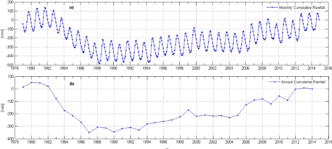
109
from hydrological models and also to fully utilize GRACE observations for the inter-annual
110
variations of TWS and water balance studies (see, Wouters et al., 2014, and the references
111
therein). While few hydrological studies that utilized GRACE data in West Africa (see, e.g.,
112
Ndehedehe et al.,2016a;Grippa et al.,2011;Hinderer et al.,2009) have been reported, some
113
drought studies and extreme rainfall conditions have also been documented in other sub-regions
114
of West Africa (see, e.g., Ali and Lebel, 2009; Ndehedehe et al., 2016b; Masih et al., 2014;
115
Bader and Latif, 2011; Nicholson et al., 2000; Nicholson, 2013, and the references therein).
116
Despite the progress made so far in the use of GRACE data in hydrological studies, for instance,
117
applications in drought and flood estimation (e.g., Reager et al., 2014; Yirdaw et al.,2008),
118
the potential of GRACE data in monitoring the space-time development of TWS changes and
119
droughts in the LCB are yet to be fully explored.
120
In this study, we capitalize on GRACE observations to estimate the TWS over the LCB,
121
in addition to satellite altimetry-derived water levels and other hydrological variables such as
122
rainfall, and soil moisture to monitor water storage changes and the spatio-temporal
character-123
istics of droughts. Contrary to previous studies that have analysed spatio-temporal drought
124
events in other regions of the world (see, e.g., Bazrafshan et al., 2014; Santos et al., 2010;
125
Bonaccorso et al., 2003) using principal component analysis (e.g., Jolliffe, 2002), we employ
126
independent component analysis (ICA, see, e.g., Cardoso,1999;Common,1994;Cardoso and 127
Souloumiac, 1993), a higher order statistical method to localize drought patterns and
time-128
1
variable hydrological signals (i.e., TWS). Unlike in the Volta basin where the influence of
129
low frequency climate oscillations on hydrological drought was reported by Ndehedehe et al. 130
(2016b), here, the Lake Chad basin (a semi-arid Sahelian environment) is adopted as a
ten-131
tative test bed, primarily to demonstrate the use of a fourth-order cumulant statistics such
132
as the ICA to analyze spatio-temporal evolutions of drought indices at different time scales
133
(3, 6, and 12 months aggregation), and to examine the relationship of other climate modes
134
(i.e., ENSO, AMO, and AMM), which were not considered with drought temporal evolutions
135
in the Volta basin. Such analysis is essential not only in understanding drought variability,
136
but also the causes of rainfall variability, which though unclear has been somewhat associated
137
with sea surface temperature anomalies of the nearby Oceans (e.g., Bader and Latif, 2011).
138
For the drought analysis, we used the recently introduced standardised non-parametric
uni-139
variate and multivariate drought indices (see, Hao and AghaKouchak,2013,2014;Farahmand 140
and AghaKouchak, 2015) for the characterisation of different droughts (e.g., meteorological,
141
agricultural, and hydrological) over LCB. The ICA technique was employed to statistically
142
decompose SPI and standardised soil moisture index (SSI) values into spatial and temporal
143
patterns while the multivariate standardised index (MSDI), was used to evaluate the
effective-144
ness of two climate variables (rainfall and soil moisture) in capturing drought properties such
145
as frequency, persistence, and termination. This study specifically aims at (i) localising and
146
characterising spatio-temporal evolutions of drought patterns over the LCB and (ii) identifying
147
spatial variability of TWS changes and the estimation of trends in lake height variations over
148
the LCB.
149
While we provide background information on the spatio-temporal variability of drought
150
patterns in Section2, further details on the method and the results of the study are presented
151
in Sections 3 and 4, respectively.
152
2. Spatio-temporal Variability of Drought 153
The lack of in-situ measurements to assist in hydrological monitoring limits the prospects
154
of a robust, large scale monitoring of major hydrological variables (i.e., rainfall, water levels,
155
groundwater, and river discharge) in the LCB. Standard routine measurements of these
hy-156
drological quantities are lacking due to limited gauge stations and deterioration of existing
157
hydrological facilities. Although local measurements from dedicated regional networks such
158
as the African Monsoon Multidisciplinary Analysis-Couplage de l’Atmosph`ere Tropicale et du
159
Cycle Hydrologique (AMMA-CATCH, Lebel et al.,2009) hydro-meteorological observing
Kainji
Figure 1: Study area showing Lake Chad, the riparian countries that constitute the Lake Chad basin, and important river networks (blue line) within the basin. Our analysis focuses on the conventional basin area (a subset of the blue polygon), which includes mostly southern and north eastern sections of Niger, Chad, north-eastern Nigeria, northern Cameroon, and most parts of Central African Republic. Maps are adapted from www.worldmap.org and http://assets.panda.org/img/original/chadmap.gif. The LCB lies at the south western crossroads of the Sahel and forest savanna, a transition zone between the Sahara Desert and the tropical savanna of West Africa (Okonkwo et al.,2013).
tem have been used in some studies (e.g., Gosset et al.,2013), the AMMA-CATCH networks
161
are highly insufficient for a regional study as they are only available in few countries (i.e.,
162
Niger, Mali, and Benin). Further, while most available data cannot be accessed by the public
163
and relevant research institutions as a result of government policies and bureaucracies, political
164
instability in the sub-regions complicates efforts to acquire such data. In addition, incomplete
165
data records and gaps in available data tend to affect proper assessment and monitoring of
166
hydrological conditions in the region.
167
However, with the plethora of available climate data either in the form of satellite
obser-168
vations or model-generated products, monitoring hydro-climatic conditions is somewhat not
169
difficult. The critical issues have often revolved around the understanding and localisation of
170
these multiple and growing climate signals. For instance, the use of mean standardised
precip-171
itation index (SPI, McKee et al.,1993) time series in estimating drought conditions over the
172
Sahel has not been very effective. This is because of the influence of strong spatial variability
1973
1987
2003
2013
Cameroon Central African Republic Nigeria Chad Lake Chad Niger Northern pool Southern poolChari River
Figure 2: The spatial and temporal changes in Lake Chad surface area as shown by Landsat imageries for 1973, 1987, 2003, and 2013. The Chari river, which provides about 95% of the inflow to the Lake is indicated. The blue lines on the map (left) show the river networks within the basin most of which constitute the Chari river system. The present Lake Chad show two segmented pools with the northern pool completely dried up during drought periods (right). Maps and imageries are adapted from (i) www-stud.informatik.uni-frankfurt.de/sfb268/d6/pics/misc/franke2000gr-abb1-gross.gif and (ii) United States geo-logical surveys (http://earthshots.usgs.gov/earthshots/Lake-Chad-West-Africa).
of rainfall at annual scale and the mean inter-annual climatological gradients across the region
174
(Ali and Lebel, 2009). Schewe et al. (2013) described the signal problem more succinctly,
175
indicating that at regional scales, the projections of climate models for instance, in terms
176
of precipitation patterns and magnitudes, are inconsistent when compared to global average
177
changes. This unavoidably leads to uncertainties in the attempt to understand the effect of
178
climate change on water resources at regional scales. In West Africa, Ali and Lebel (2009)
179
reported that despite the significantly dry season of 2006, working with a rainfall product with
180
spatial resolution of 0.5◦ x 0.5◦ resulted in only 28% of the area being significantly dried while
181
15% of the Sahel region was significantly wet. They also observed that SPI on a 1◦ x 1◦ grid
182
in the Sahel was not representative of the whole region. Irrespective of the spatial resolution
183
of the data and differences in climatic zones, drought analysis from a spatio-temporal point of
view can improve our understanding of drought occurrence. One approach to spatio-temporal
185
drought analysis would be the use of a component extraction technique, in particular,
prin-186
cipal component analysis (PCA, Jolliffe, 2002). For example, Bazrafshan et al. (2014) in a
187
recent study reported on the multivariate approach, which uses the PCA of the SPI time series
188
in capturing the temporal variability of drought patterns at different time scales (i.e., 3, 6,
189
and 12 month scale) while Bonaccorso et al. (2003) studied long-term drought variability in
190
Sicily during 1926-1996 period using the PCA technique. Further, using PCA and K-means
191
clustering,Santos et al.(2010) was able to show that the south of Portugal had more frequent
192
cycles of dry events (every 3.6 years) than the northern part where severe to extreme droughts
193
occurred approximately every 13.4 years. Following the strong spatial variability of rainfall
194
in the Sahel region where LCB is located, our approach uses a regionalisation process where
195
the decomposed SPI time series from PCA are rotated towards statistical independence, a
196
process referred to as independent component analysis (e.g.,Aires et al.,2002;Cardoso,1999;
197
Cardoso and Souloumiac, 1993). Our approach differs from the aforementioned studies in
198
that the derived SPI time series, which are based on a non-parametric approach derived from
199
the empirical probability method (see Farahmand and AghaKouchak,2015;Hao and AghaK-200
ouchak,2014) are decomposed through a classical rotation of the PCA modes. This is done in
201
a way to enable the localisation and extraction of physically meaningful drought signals that
202
are statistically significant. The use of a regionalization method such as the ICA enables the
203
localization of SPI and standardised soil moisture index (SSI) signals in terms of its spatial
204
variability and temporal evolutions in the basin. This approach is useful in understanding
205
the space-time evolution of extreme rainfall and soil moisture conditions in the basin. For
206
an endorheic basin such as the LCB, which lacks a suitable framework to monitor space-time
207
occurrence of drought, this approach to drought monitoring, when integrated with the
analy-208
sis of changes in TWS and altimetry derived water levels of Lake Chad, largely supports the
209
assessment of available water resources. We provide more details on the ICA technique in
210
Section 3.
211
Moreover, in this study, we hypothesized that following the dramatic decline and
desicca-212
tion of Lake Chad surface area due to strong precipitation deficit of the 1980’s (see cumulative
213
rainfall anomalies, Fig. 3), meteorological drought propagates into both agricultural and
hy-214
drological droughts with strong impact on the catchment stores (i.e., lakes, rivers, soil water,
215
and aquifers). Several drought studies have associated hydrological drought with precipitation
216
deficit on a longer time scale such as 6, 12, and 24 months (see, e.g., Li and Rodell, 2015;
Santos et al.,2010;Vicente-Serrano,2006;Rouault and Richard,2003;Hayes et al.,1999; Ko-218
muscu,1999). In sum, we used precipitation and soil moisture data, covering a 35-year period
219
to quantify drought frequency (how often a drought event occurs) and severity (the intensity
220
or strength of a drought event) for all drought categories (meteorological, agricultural, and
221
hydrological).
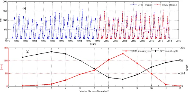
Figure 3: Cumulative rainfall anomalies averaged over LCB using the GPCP based precipitation. (a) Monthly cumulative rainfall anomaly over the basin during 1979-2014 period. (b) Annual cumulative rainfall anomaly over the basin during 1979-2014 period.
222
3. Data and Method 223
3.1. Data 224
3.1.1. GRACE-Derived Terrestrial Water Storage (TWS) Changes 225
Gravity Recovery and Climate Experiment (GRACE, Tapley et al., 2004) Release-05
226
(RL05) spherical harmonic coefficients from Center for Space Research (CSR) for the period
227
of April 2002 to October 2014 were used in this study to compute changes in TWS. The CSR
228
RL05 gravity field solutions, which are truncated at degree and order 60 were retrieved from the
229
open access files available at http://icgem.gfz-potsdam.de/ICGEM/shms/monthly/csr-rl05/.
230
These spherical harmonic coefficients suffer from signal attenuation and satellite measurement
231
errors leading to noise in the higher degree coefficients (Landerer and Swenson,2012;Swenson 232
and Wahr,2002). As a first step in the processing, the degree 2 coefficients were replaced with
233
estimates from satellite laser ranging (Cheng et al.,2013) while the degree 1 coefficients
pro-234
vided by Swenson et al.(2008) were used. This was necessary since GRACE does not provide
changes in degree 1 coefficients (i.e., C10,C11, and S11), and is also affected by large tide-like
236
aliases in the degree 2 coefficients (i.e., C20). Secondly, after removing the long term mean,
237
DDK2 de-correlation filter (Kusche, 2007) was applied on the GRACE monthly solutions in
238
order to reduce the effect of correlated noise. Practically, non-isotropic filters such as the
239
DDK2 (Kusche, 2007) accommodate better the GRACE error structure when compared to
240
the conventional isotropic Gaussian filter (see, e.g., Werth et al.,2009). We point out briefly
241
that there are no standard filtering procedures as most GRACE users would largely prefer
242
the most convenient and easy-to-implement approaches. However, the filtering process can
243
be significantly improved by using decorrelation filters, which unlike the Gaussian filter, fits
244
better the noise in the data (e.g., Belda et al., 2015). The filtered monthly solutions were
245
then converted to equivalent water heights on a 1◦ x 1◦ grid using the approach ofWahr et al. 246 (1998): 247 4W(φ, λ, ξ) = Rρave 3%w lmax X l=0 2l+ 1 1 +kl l X m=−l Plm(φ, λ)4Ylm(ξ) (1)
where4W is equivalent water height (hereafter TWS) for each month in time (ξ), and where
248
φand λare the latitudes and longitudes, respectively. Ris the mean radius of the Earth (i.e.,
249
6378.137 km),ρave is the average density of the Earth (5515kg/m3),%w is the average density
250
of water (1000kg/m3),klis the load Love numbers of degreel,Plmare the normalized spherical
251
harmonic functions of degreeland ordermwithlmax=60 and4Ylmare the normalized complex
252
spherical harmonic coefficients after subtracting the long term mean. Since the effect of the
253
DDk2 filter whose radius coincides with 340 km of the Gaussian filter leads to attenuation of
254
the signal amplitude (e.g., Wouters and Schrama, 2007; Baur et al., 2009), a scaling factor
255
obtained from Global Land Data Assimilation System (GLDAS, Rodell et al., 2004) derived
256
terrestrial water storage content (see details in Section 3.1.7) was computed in a manner
257
similar to Landerer and Swenson (2012). This scaling factor was applied to the
GRACE-258
derived TWS values in order to restore the geophysical signal loss caused by the impact of the
259
DDK2 decorrelation filter. Apparently, the use of GRACE data has progressed in the direction
260
of full scale hydrological applications and water resources monitoring (seeWouters et al.,2014).
261
Thus, accounting for the effect of the filter in the transformed GRACE observations becomes
262
essential as the signal attenuation will become an error in the residual in regional water balance
263
or might serve as a constraint in water budget closure (seeLanderer and Swenson,2012). The
264
rescaled monthly TWS grids had a few random gaps of up to 12 months in between that were
265
filled through interpolation. This is particularly important for the regionalisation process,
which requires continuous spatio-temporal data.
267
3.1.2. Tropical Rainfall Measuring Mission (TRMM) Data 268
Rainfall observations from TRMM 3B43 (Huffman et al., 2007; Kummerow et al., 2000)
269
provide good estimates of rainfall magnitude not detected by other satellite precipitation
270
products. In West Africa for example, Nicholson (2013) had reported that TRMM
valida-271
tion using in-situ data showed zero bias, having a root mean square error (RMSE) of 0.7
272
and 0.9 mm/day for the seasonal and August rainfall, respectively. Specifically, TRMM
273
3B43 version 7, which has a global coverage (i.e., 50◦S and 50◦N) provides monthly
pre-274
cipitation estimates at a spatial resolution of 0.25◦ x 0.25◦ and has been significantly
im-275
proved (e.g., Duan and Bastiaanssen, 2013b). Due to its spatial resolution and bias with
276
in-situ observations, we used TRMM 3B43 to estimate monthly and seasonal rainfall in the
277
LCB. The data covering the period 1998-2013 was used and is available at the National
278
Aerospace and Space Administration (NASA) Goddard Space Flight Center (GSFC) website
279
(http://disc.gsfc.nasa.gov/datacollection/TRMM3B43-V7.shtml).
280
3.1.3. Global Precipitation Climatology Project (GPCP) 281
The 2.5◦ x 2.5◦ global grids of monthly estimate from GPCP version 2.2 precipitation
282
data set (e.g., Huffman et al., 2009; Adler et al., 2003) is a merged satellite-based product
283
(includes satellite microwave and infrared data) that is adjusted by the use of rain gauge
284
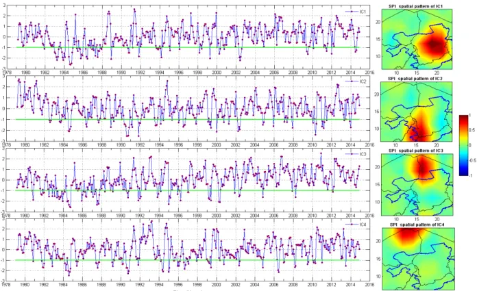
analysis. Unlike Ethiopia and some other countries in East Africa where TRMM is
com-285
pletely inconsistent with GPCP (Paeth et al., 2012), the GPCP rainfall product is highly
286
correlated and consistent with TRMM in the region and is used here for the spatio-temporal
287
analysis of drought in the LCB. The GPCP version 2.2 data, covering the period of
1979-288
2015, was used since drought analysis using SPI requires data record of at least 30 years.
289
The archived data is distributed through World Data Center and is available for download at
290
http://lwf.ncdc.noaa.gov/oa/wmo/wdcamet-ncdc.html.
291
3.1.4. Satellite Altimetry Water Level Variations 292
Lake level height variations computed from TOPEX/POSEIDON (T/P), Jason-1 and
293
Jason-2/OSTM altimetry provided by the United States Department of Agriculture (USDA)
294
was used to study Lake Chad surface water. The data covering the period 1993 to 2015 was
295
downloaded from www.pecad.fas.usda.gov/cropexplorer/globalreservoir and used to analyse
296
water level variations. The time series of USDA monthly lake height variation used for the
study have been smoothed with a median type filter in order to eliminate outliers and reduce
298
high frequency noise. The use of altimetry-based measurements for a data deficient region
299
such as the LCB, as stated by Coe and Birkett(2004), is beneficial since they are continuous
300
and potentially available few days after measurement. That is quite unlike gauge data that
301
are irregular and difficult to acquire due to government policies and bureaucracies.
302
3.1.5. Climate Prediction Center (CPC) Soil Moisture 303
The monthly CPC soil moisture data version 2 (Fan and Dool, 2004) with spatial
reso-304
lution of 0.5◦ x 0.5◦ for the period between 1979 to 2014 was used in this study to
inves-305
tigate water availability through standardised soil moisture index (SSI). The data, which is
306
model-based is derived from monthly global rainfall data that uses more than 17000 rain
307
gauges worldwide and monthly global temperature from reanalysis. In addition, the data
308
has been used to extract climate teleconnection patterns such as the El-Ni˜no Southern
Os-309
cillation and long term trends (Fan and Dool, 2004). The data is freely available at NOAA
310
(http://www.esrl.noaa.gov/psd/data/gridded/data.cpcsoil.html) for download.
311
3.1.6. Climate Indices 312
Relevant and well known global climate teleconnections indices such as El-Ni˜no Southern
313
Oscillation (ENSO), Atlantic Multi-decadal Oscillation (AMO), and Atlantic Meridional Mode
314
(AMM) have been associated with precipitation patterns (see, e.g., Giannini et al., 2003;
315
Nicholson, 2013; Giannini et al., 2013; Paeth et al., 2012), important factors that regulate
316
the formation and persistence of drought events in the Sahel and some countries of West
317
Africa. These indices, covering the period 1979-2014, were used to examine the relationship and
318
possible links of observed temporal evolutions of droughts in LCB with coupled
atmosphere-319
ocean system and perturbations of nearby oceans. We point out briefly that other ENSO
320
indices such as Nino3.4 and Nino4.0 exist but we used Multivariate Enso Index-MEI (hereafter
321
called ENSO) since it comprises six other variables over the Pacific coupled with atmospheric
322
anomalies. The climate indices used in this study can be downloaded from National Oceanic
323
& Atmospheric Administration (NOAA) websites (e.g., http://www.cpc.ncep.noaa.gov).
324
3.1.7. Global Land Data Assimilation System (GLDAS) 325
GLDAS (Rodell et al., 2004) derived monthly total water storage content (TWSC) at
326
1◦ x 1◦ spatial resolution was used to rescale the GRACE-derived TWS change in order to
327
remedy the signal loss due to filtering. GLDAS is unique because it integrates both satellite
and in-situ data to produce optimal fields of land surface states and fluxes (Rodell et al.,
329
2004). The TWSC was derived from summing all the layers from Noah 2.7.1 land surface
330
model of GLDAS (i.e., all the soil moisture layers including the canopy water storage). This
331
land surface model (i.e., the NOAH component of GLDAS) showed a good agreement with
332
GRACE-derived TWS in West Africa, indicating a coefficient of determination (R2) of 0.85
333
(Ndehedehe et al., 2016a). However, the averaged TWSC and GRACE-derived TWS in the
334
LCB showed a relatively stronger agreement (i.e., R2 of 0.88) with a root mean square
er-335
ror of 19.83 (see Appendix A3, Fig. 17). While it is important to acknowledge that the
336
GLDAS model incorporates soil moisture and plant canopy surface water storage, it does not
337
include surface and groundwater components. However, previous studies have reported a good
338
agreement between GLDAS-TWSC and GRACE-derived TWS at basin scale (e.g.,Moore and 339
Williams,2014). To derive the scale factor, TWSC was filtered using the DDK2 filter similar
340
to GRACE observations. Thereafter, the ratio of the DDK2 filtered TWSC to the unfiltered
341
and synthesised TWSC was used to derive a scale factor. This scale factor, which measures
342
the impact of DDK2 filter on GRACE-observations, was then applied to the gridded TWS
343
values similar to previous studies (see, e.g., Long et al., 2015; Landerer and Swenson,2012).
344
GLDAS-derived TWSC covering the years 2001-2014 was obtained from the open access file
345
available at http://grace.jpl.nasa.gov/data/get-data/land-water-content/.
346
3.1.8. Sea Surface Temperature (SST) 347
SST version 2 (Reynolds et al.,2002) data was downloaded from the website (http://www.es
348
rl.noaa.gov/psd/data/gridded/data.noaa.oisst.v2.html) of the National Oceanic and
Atmo-349
spheric Administration (NOAA). The period covered is from 2002 to 2014. The SST averaged
350
of the Atlantic Ocean (30◦S−30◦N and 70◦W−20◦E) was used in this study to investigate its
351
relationship with annual cycles of rainfall over the basin.
352
3.1.9. Satellite Image Analysis 353
Landsat 7 Enhanced Thematic Mapper plus (ETM+) and Landsat 8 imageries were
down-354
loaded from the United States geological surveys website (http://glovis.usgs.gov/). The
im-355
ageries for 2000, 2003, and 2015 in the Lake Chad area were clipped and classified using
356
Iterative Self-Organizing Data Analysis Technique Algorithm (ISoData) technique proposed
357
by Ball and Hall (1965). The method is an unsupervised classification method that uses an
358
iterative clustering algorithm and allows the number of clusters to be dynamically determined.
359
The surface area of the Lake at different epoch was estimated using the classified pixels
resenting water bodies. Estimating the recent surface area is critical to understanding the
361
desiccation story of the basin in recent times. It is also important to evaluate the wet/dry
362
regimes of the basin in the last decade.
363
3.2. Method 364
3.2.1. Standardised Drought Indices 365
Drought phenomenon is usually expressed using standardised indices for example,
stan-366
dardised precipitation index (SPI, McKee et al.,1993) and standardised runoff index (Shukla 367
and Wood,2008) amongst others. The SPI is a very popular drought index. It is normalized
368
so that wetter and drier climates can be represented in a similar way and can be calculated
369
for other water variables and hydrological quantities such as snowpack, reservoir, streamflow,
370
soil moisture, and ground water (McKee et al.,1993). In this study, we utilised two variables
371
(rainfall and CPC model soil moisture) to implement a non-parametric standardised
multivari-372
ate drought index in order to compensate for the weakness of single drought index as argued
373
by Hao and AghaKouchak(2014). The mathematical framework of this non-parametric
mul-374
tivariate standardised drought index (MSDI) and other single drought indicators (e.g., SPI
375
and SSI) is fully documented by Farahmand and AghaKouchak (2015). These drought
in-376
dicators adopt empirical method to determine the marginal probability of precipitation and
377
other variables such as soil moisture, evapotranspiration, and runoff. The MSDI combines
378
two hydrological quantities to derive a composite drought index, which can be described as
379
a multivariate prototype of the popular SPI (AghaKouchak,2015). Recently, the MSDI has
380
been shown to be a statistically consistent drought index (Huang et al.,2015) and is employed
381
here for the first time in the region. The joint distribution of two variables X and Y expressed
382
as (Hao and AghaKouchak,2013)
383
P(X≤x, Y ≤y) =p, (2)
where p represents the joint probability of any two variable (e.g., rainfall and soil moisture).
384
The joint probability is then used to define the MSDI as
385
M SDI =φ−1(p) (3)
whereφ−1 is the standard normal distribution function. For the bivariate case, the Gringorten
386
plotting position formula (see Farahmand and AghaKouchak, 2015;Hao and AghaKouchak,
387
2014) is used to estimate the empirical joint probability. The empirical Gringorten plotting
388
position is expressed as:
p(xk, yk) =
mk−0.44
n+ 0.12 , (4)
wherenis the number of the observation andmkis the number of times which the pair (xi, yi)
390
occur forxi≤xk andyi ≤yk (1≤i≤n). Eq. 4 is used in Eq. 3to compute the MSDI while
391
the standardised precipitation index (SPI) and standardised soil moisture index (SSI) are also
392
estimated using the univariate form of Eq. 4. Thus, we combined averaged GPCP rainfall and
393
soil moisture to derive time series of MSDI, in addition to the single drought indicators across
394
different time scales (i.e., 1, 3, 6, and 12 months). The drought classification and extreme
395
rainfall events used in this study are based on the description of McKee et al. (1993) (Table
396 1).
397
As discussed earlier in Section2, localising drought signals has been a major limitation in
398
drought studies. Hence, the ICA method (see details in Section 3.2.2) was used to decompose
399
the gridded time series of computed SPI and SSI at 3, 6, and 12 month scales into independent
400
modes (i.e., temporal and spatial patterns) where drought/wet signals are localised in terms
401
of their spatial and temporal variations. The statistically significant modes of variability
402
identified in the LCB were analysed further. Essentially, this statistical decomposition of
403
meteorological and land surface state variables (i.e., rainfall and soil moisture) into spatial and
404
temporal patterns allow the extraction of climate teleconnection patterns and other relevant
405
coupled ocean atmosphere patterns that are related to the observed wet and dry periods in the
406
basin. Prior to decomposing gridded rainfall and soil moisture drought indicators into spatial
407
and temporal patterns, the spatially averaged time series of each of the two datasets were used
408
to compute time series of SPI and SSI. That provides the opportunity to compare the results
409
of the two approaches (i.e., the decomposed gridded drought indicators and time series of
410
averaged indicators over the basin). To understand the relationship of climate teleconnection
411
indices with ICA-derived temporal variability of drought patterns, Pearson correlation analysis
412
was applied. The SPI values at 3, 6, and 12 month scales for all first and second ICA modes,
413
were selected for this correlation with global climate teleconnection indices (i.e., AMO, AMM,
414
and MEI). This choice is based on the theoretical assumption that the first and second ICA
415
modes have relatively stronger dominant modes of variability. A student T-test was then used
416
to calculate the significance of the correlation at 95% confidence level.
Table 1: Drought classification and extreme rainfall/soil moisture events based onMcKee et al.(1993) classifi-cation system.
Description Threshold Extreme wet +2.0 and above Very wet +1.5 to +1.99 Moderately wet +1.0 to +1.49 Near normal -0.99 to +0.99 Moderate drought -1.0 to -1.49 Severe drought -1.5 to -1.99 Extreme drought -2.0 or less
3.2.2. Independent Component Analysis (ICA) 418
The ICA (see, e.g.,Ziehe,2005;Cardoso and Souloumiac,1993;Cardoso,1991;Common,
419
1994; Cardoso,1999) technique (see further details in Appendix A2) was used to decompose
420
a data matrix X, into spatial maps M, and temporal patterns T, as:
421
XSP I/SSI/T W S(x, y, t) =TM, (5)
where (x, y) are grid locations, t is the time in months. T is unit-less since it has been
nor-422
malised using its standard deviation while the corresponding spatial patterns M, have been
423
scaled using the standard deviation of its independent components (i.e.,T). In this study, we
424
used the JADE (see further details in Appendix A2) algorithm (available at
http://perso.telecom-425
paristech.fr/cardoso/Algo/Jade/jadeR.m) to decompose standardised drought indicators (i.e.,
426
the gridded SPI and SSI data) and GRACE-derived TWS into spatial maps and temporal
427
patterns. Each ICA mode (a pair of the independent components and spatial patterns) of
428
variability is a combination of the temporal and spatial patterns and are usually interpreted
429
together (i.e., the unit-less temporal evolution is multiplied with the spatial pattern in order
430
to obtain the actual values of SPI, SSI, and TWS).
431
3.2.3. Trends and Correlation Analysis 432
The trends in observed temporal evolutions of TWS and Lake Chad water level variations
433
were estimated using the least squares method. Further, we examined the relationship of
434
climate teleconnections with observed temporal SPI patterns (i.e., at 3, 6, and 12 months
ag-435
gregation) using the linear correlation coefficient (r). The significance of observed correlations
were tested at 95% confidence level using the Student-t distribution test as 437 t=r r n−2 1−r2, (6)
where nis the total number of given observations for the data.
Figure 4: Averaged monthly rainfall over Lake Chad basin and annual cycles of TRMM-based precipitation and sea surface temperature (SST). (a) Time series of spatially averaged rainfall over Lake Chad basin using GPCP version 2.2 (1979−2013) and TRMM 3B43 based precipitation (1998−2013) (b) Long term mean annual cycle of rainfall over Lake Chad basin using TRMM 3B43 based precipitation and annual cycle of SST data averaged over the Atlantic Ocean (30◦S−30◦N and 70◦W−20◦E).
438
4. Results and Discussions 439
4.1. Seasonal Rainfall Patterns over the Lake Chad Basin (LCB) 440
TRMM 3B43 version 7 precipitation product was used for the seasonal analysis and long
441
term annual cycle while the GPCP version 2.2 precipitation data was used for the drought
442
analysis because of its duration (35 years). A 35-year data meets the criteria for SPI since a
443
30-year data or less shortens the sample size and undermines the confidence in its usage (e.g.,
444
Svoboda et al.,2012). Comparing the TRMM and GPCP based precipitation products, the
445
spatially averaged GPCP product was consistent (indicated a linear correlation of 0.99) with
446
the spatially averaged TRMM product. This near-perfect correlation is expected since TRMM
447
is adjusted by rain gauge observations, most of which are included in the GPCP datasets.
448
Despite the differences in the spatial resolutions of these two precipitation products, their
449
strong agreement over the LCB can be useful in future studies to characterise uncertainties in
water budget analysis. Although no notable trend is observed in the spatially averaged rainfall
451
over the basin, we observe a recent pronounced maximum peak in 2012 that is similar to other
452
extreme wet years, for example, 1988, 1994, 1999, 2003, and 2006 (Fig.4a). The lowest annual
453
rainfall peak observed in 1984 (Fig.4a) is consistent with the well known drought that ravaged
454
the African continent during the 1982-1984 period (e.g.,Masih et al.,2014). The annual cycle
455
of precipitation over LCB indicates a peak in August while the seasonality of SST shows an
456
opposite phase with rainfall (Fig. 4b). Most parts of the LCB lies in the Sahel region, and
457
the impact of SST variability on rainfall has been reported (Mohino et al.,2011;Paeth et al.,
458
2012; Lebel and Ali, 2009). Rainfall decline in the coastal West African countries has been
459
associated with cold SST along the Atlantic and warm SST in the eastern tropical Pacific while
460
decadal rainfall trends in the Sahel is assumed to be influenced by a combination of multiple
461
low-frequency SST signals (e.g., Rodrguez-Fonseca et al.,2011).
462
Moreover, the seasonal analysis show that maximum rainfall (temporal variations) comes
463
between July and September with a maximum averaged rainfall of about 150 mm while other
464
seasons have less than a 100 mm of rainfall (Fig.5, right). The spatial distribution of rainfall
465
indicates a maximum of about 250 mm of rainfall towards the southern part of the basin
466
and more than 300 mm outside the conventional basin area (Fig. 5, left). Comparatively, the
467
GPCP version 2 seasonal rainfall patterns over the basin also show similar temporal and spatial
468
patterns with the July-September period indicating relatively low pronounced amplitudes of
469
rainfall (e.g., 1983−1984, 1987, etc.) in the temporal variations due to extreme drought
470
conditions (see Appendix A1, Fig. 16). Generally, the July-September rainfall (i.e., using the
471
GPCP data) in the basin is the dominant rainfall as the most pronounced maximum peaks
472
correspond to those of Fig. 5. Overall, the seasonal rainfall patterns over the basin, clearly
473
show the dichotomy between the northern section (having low rainfall) and the southern band
474
(which receives more rainfall especially between July and September) (Fig. 5). This seasonal
475
picture of rainfall in the basin is crucial as it has the capacity to enhance the assessment of
476
the basin’s hydrology. The knowledge of the basin’s climatology, in terms of seasonal rainfall
477
can enhance our interpretation of the standardised drought indices.
478
4.2. Drought Characteristics Over the Lake Chad Basin (LCB) 479
4.2.1. Time Series of Standardised Drought Indicators 480
The standardised drought indicators (i.e., SPI, SSI, and MSDI) for the LCB were computed
481
at 1, 3, 6, and 12 month cumulations using spatially averaged GPCP and CPC soil moisture
Figure 5: Seasonal rainfall analysis for Lake Chad Basin (5.5◦N-24.5◦N and 5.5◦E-24.5◦E) using TRMM satellite data for the period 1998−2013. Spatial patterns (left) and temporal patterns (right) are averaged over the geographical boundary describing the spatial extent of Lake Chad basin used in this study. The inset (i.e., the solid black line) is the conventional basin boundary.
data over the basin. Results show that shorter time scales (e.g., 1 and 3 month cumulations)
483
have high drought frequencies (Fig. 6a-b). The frequency reduces with increase of time scales
484
(e.g., 6 and 12 month cumulations) (Fig. 6c-d). According to Komuscu (1999), this kind of
485
relationship implies that the index responds more slowly as the time scales increases.
Con-486
sistent decrease in SPI and MSDI values were observed from 1979 to 1985 (Fig. 6) but with
487
recovery in 1984 at 3 and 6 months scale. The strong decline of SPI and MSDI within this
488
period coincides with the hydrological drought record of the basin, which showed a dramatic
489
loss of 15138 km2 in the surface area of Lake Chad (see, Alfa et al., 2008). The MSDI and
490
SSI show drought persistence in 1990/1991 at all scales (Fig. 6a-d); 1998 at 3 and 6 months
491
(Fig. 6b-c); and 2009 at 6 and 12 months (Fig. 6c-d). The drought years as indicated in the
standardised drought indicators are generally consistent with observed decline in the northern
493
pool of the Lake as previously reported by Lemoalle et al.(2012). In addition, the observed
494
wet (e.g., 1988 and 1994) and dry (e.g., 1983−1985) years (Fig. 6) are consistent with the
495
records of observed water levels at Kindjeria (i.e., at the northern section of LCB) as reported
496
in a previous study by Lemoalle et al.(2012). They noted that the northern pool gets flooded
497
during extreme wet periods and completely dry for several years due to incessant drought
con-498
ditions. Similar patterns in the behaviour of surface waters (e.g., Lakes) vis-`a-vis drought and
Figure 6: Time series of standardised drought indicators (i.e., SPI, SSI, and MSDI) for Lake Chad basin using averaged GPCP and CPC soil moisture data covering the period 1979−2013 (i.e., over the basin). The MSDI is derived through the combination of GPCP based precipitation and CPC based soil moisture data. These standardised drought indicators are based on empirical probability, different from the gamma distribution function used in the SPI case ofMcKee et al.(1993).
499
wet periods in the region have been reported (e.g., Bekoe and Logah,2013; Lemoalle et al.,
500
2012). Also, previous studies have associated the decline in the surface area of the lake to
501
human activities (e.g., water use for irrigation) and the impact of climate variability (see, e.g.,
502
Coe and Foley,2001;Gbuyiro et al.,2001). Some of the drought cases identified in the study
503
(i.e., using averaged SPI) are somewhat generalised and appear not to be very massive (i.e., in
terms of severity). But the cases are significant enough to impact negatively on the agrarian
505
system and food security conditions of the basin where agriculture is predominantly rain-fed.
506
Furthermore, extreme wet conditions in 1987/1988 (all through the year), and 1994/1995
507
show strong persistence in wetness by SSI (Fig.6a-d). On the contrary, SPI and MSDI showed
508
drought conditions in 1987 while in 1995 they indicated that the wet conditions actually ended,
509
unlike SSI, which indicated that the severe wet conditions that started in late 1994 persisted
510
even till 1996 (Fig. 6b-d). This inconsistency is probably caused by intense rainfall occurring
511
within few months while the remaining months of the year are consistently dry. The SPI
512
values (i.e., at 1 and 3 months cumulation) tend to be very high during the 2003−2013 period
513
(Fig.6a-b), and are consistent with the findings ofOkonkwo et al.(2013) whose report showed
514
increase in SPI values between 2002 and 2011 in the basin. However, the SSI and MSDI
515
show longer drought durations in late 2004 (Fig. 6a-b) and 2005 (Fig.6c-d). In the drought
516
assessment done so far using the three standardised indicators over the LCB, recent conditions
517
of wetness in late 2010 and 2012/2013 captured by SPI, SSI, and MSDI (Fig. 6a-d) appear to
518
be a dramatic deviation from the long string of frequent drought conditions observed in the
519
basin (note that at 12 month cumulation period, only SPI indicated wet condition in 2010 while
520
SSI and MSDI showed a recovery from drought condition). This period (i.e., between 2010
521
and 2013), which also coincides with increased water level in Lake Chad as shown in Section
522
4, is largely consistent with the spatially averaged rainfall over the basin within the same
523
period (Fig. 4a). Further, as the accumulation period increases (i.e., for SPI), soil moisture
524
conditions tend to respond slowly to extreme wet conditions of SPI. It seems that the extreme
525
wet condition was not sufficient enough to cushion the deficit conditions of soil moisture in the
526
basin. For instance, when we evaluate SPI (i.e., 12 month scale) values of 1991, 2006−2007
527
and 2012−2013 periods against SSI and MSDI (i.e., 12 month scale) values during the same
528
period, the inconsistencies are rather obvious. SPI indicates extreme wet conditions during
529
those periods (1991/1992 and 2006−2007) while MSDI and SSI show extreme drought (1991
530
and 2006 −2007) and normal conditions (2011−2013 period) as against the extreme wet
531
condition indicated by the SPI (2012−2013 period) (Fig. 6). Soil moisture deficits have been
532
related to antecedent conditions, evaporation, seepage to groundwater, evapotranspiration,
533
and runoff (e.g., Loon, 2015). According to Birkett (2000), Lake Chad loses about 80% of
534
water through evaporation due to low humidity and high temperatures. Considering the fact
535
that the basin is located in a semi-arid Sahelian environment, these factors and others (e.g.,
536
soil characteristics) may account for the observed inconsistencies between SPI and SSI. In
subsequent sections we show results of the statistical decomposition of SPI and SSI signals
538
into spatial and temporal patterns using the ICA technique.
Figure 7: ICA-derived spatio-temporal SPI patterns of LCB using 3-month gridded SPI values. The SPI values are computed using GPCP rainfall product for the period 1979−2014. Localised spatial SPI patterns (right) corresponds to the temporal evolutions (left). The actual SPI values to be used for drought classification are jointly derived from the spatial and temporal SPI patterns. The green solid line is drought threshold.
539
4.2.2. Spatio-temporal Analysis of Drought Patterns for SPI 540
Unlike Section4.2.1, where the spatially averaged values of rainfall and soil moisture over
541
LCB were used to compute the standardised indicators (e.g., SPI and MSDI), here, we use,
542
the gridded values of rainfall and soil moisture to compute standardised indicators, which were
543
subsequently decomposed into temporal and spatial patterns using the ICA technique. The
544
spatial patterns are localised signals (i.e., spatial maps indicating the direction of wet/drought
545
conditions) that show spatial variability of rainfall conditions corresponding to the temporal
546
evolutions. The classification scales (e.g., extremely wet, moderately dry, severely dry,
ex-547
tremely dry) for the SPI values (see, e.g., Hayes et al.,1999; McKee et al., 1993) are jointly
548
derived from each ICA mode (i.e., a combination of the spatial and temporal patterns).
549
The spatio-temporal SPI patterns were computed for three different time scales (3, 6, and 12
550
months). In Section 4.2.1, we showed drought index at 1 month scale (i.e., in the temporal
Table 2: Correlation coefficients between temporal evolutions of SPI (i.e., 3, 6, and 12 months SPI scales) derived from the ICA process and global climate teleconnection indices. Correlation values in bold are significant at
α= 5% confidence level.
SPI Scale Independent Components
AMO AMM ENSO
3 month 1 0.31 0.30 -0.18 2 -0.13 -0.21 0.07 6 month 1 0.38 0.38 -0.22 2 -0.45 -0.33 0.18 12 month 1 0.55 0.38 -0.34 2 0.36 0.08 -0.07
Figure 8: ICA-derived spatio-temporal SPI patterns of LCB using 6-month gridded SPI values. The SPI values are computed using GPCP rainfall product for the period 1979−2014. Localised spatial SPI patterns (right) corresponds to the temporal evolutions (left). The actual SPI values to be used for drought classification are jointly derived from the spatial and temporal SPI patterns. The green solid line is drought threshold.
drought patterns), however, in this section we choose these intermediate and long term scales
552
(3, 6, and 12 months) for the spatio-temporal drought variability since they fit in well with
Figure 9: ICA-derived spatio-temporal SPI patterns of LCB using 12-month gridded SPI values. The SPI values are computed using GPCP rainfall product for the period 1979−2014. Localised spatial SPI patterns (right) corresponds to the temporal evolutions (left). The actual SPI values to be used for drought classification are jointly derived from the spatial and temporal SPI patterns. The green solid line is drought threshold.
agricultural and hydrological drought monitoring as indicated earlier in Section 2.
554
When comparing the temporal evolutions of SPI for 3 and 6 month time scales, a number
555
of similar characteristics are observed. Declining SPI values from 1980 up to 1984 and extreme
556
drought in 1984 are observed (Figs.7and8) in the central part of the conventional basin. Also
557
there is a change in drought frequency as the time scale changes. In Fig.9, drought frequency is
558
reduced when compared to Figs.7and8where drought frequencies are high. However, drought
559
persistence is higher on longer time scales than short aggregation windows (see, Figs. 7-9).
560
This is not to suggest that all cases of longer drought duration are usually related to the
561
aggregation window. SPI aggregated over longer time scales (e.g., 12 and 24 months) are
562
sometimes used in monitoring hydrological droughts (see e.g., Ndehedehe et al.,2016b;Li and 563
Rodell,2015; Lloyd-Hughes, 2012; Santos et al., 2010). But the propagation processes from
564
meteorological to hydrological drought conditions may take some time depending on the soil
565
surface conditions, which creates a lagged response (see IC1, Figs. 7-9). At all monthly SPI
566
scales, we observed relatively strong drought spatial patterns towards the north and centre
of the conventional basin area and the entire basin at large. Even though we do not observe
568
strong spatial drought patterns directly over Lake Chad, the southern part of the basin where
569
the lake receives∼95% of its alimentation via the Chari-Logone river experienced drought at 570
3 and 6 month scales (IC2 and IC4 of Figs.7and8, respectively), that is, when the SPI values
571
are jointly considered or interpreted together from the spatial and temporal patterns. From
572
their temporal evolutions (i.e., IC2 and IC4 of Figs. 7 and8 respectively), specific years such
573
as 1984, 1990, 1992/1993, 1996, 2000, 2002, and 2010 indicate similar drought characteristics,
574
which we attribute to strong deficit in rainfall in those years. Still on the conventional basin
575
area, the corresponding temporal evolution of drought spatial patterns at 12-month scale (i.e.,
576
hydrological drought) indicates extreme drought conditions, which began in 1983 and persisted
577
till 1985 (IC1, Fig.9). Similar temporal pattern is also observed in the section of the basin that
Figure 10: Influence of global climate teleconnection indices (i.e., 1979−2014) on temporal evolutions of hydrological droughts (i.e., 12 month SPI). The temporal drought pattern of ICA mode 1 shown in Fig. 9are correlated with AMO (top), AMM (middle), and MEI (bottom).
578
belongs to Niger (IC4, Fig. 9). IC2 and IC3 of Fig. 9show SPI signals in Libya and northern
579
Chad respectively. Apart from the extreme wet conditions of 1988, 1994, and 1998-1999 in
580
some parts of the LCB (IC1 and IC4, Fig. 9), which was also reported by Nicholson et al. 581
(2000), the period between late 1995 and 1997 indicates drought persistence with extreme dry
conditions in 1996/1997 at northern Chad (IC3, Fig. 9). We point out briefly that while IC1
583
of Fig. 9(i.e., Central Chad) showed extreme wet conditions in the 1988/1989 period, IC2 of
584
Fig. 9 (i.e., Libya) indicated a drought condition in 1998 with recovery in 1999. As a result,
585
Libya was more or less climatically stable (i.e., when compared to 1994, 2006, and 2012).
586
While the conventional basin area was relatively wet during 2001−2014 period (though with
587
fluctuating SPI values) (IC1 of Fig.9), drought conditions in the last decade (2001, 2009, and
588
late 2013−2014) in Libya (IC2, Fig. 9) and southern Niger (IC4, Fig. 9) demonstrate the
589
importance of a spatio-temporal approach to drought analyses. Apart from the SPI signal
590
in Libya, recent wet conditions in 2010-2013 seems to be prevalent in the basin (IC1,
IC3-591
IC4, Fig. 9) with the conventional basin area indicating mostly wet conditions since 1999
592
(IC1, Fig. 9). The observed wet and dry periods from our localised drought signals, which we
593
attribute partly to the impacts of La-Ni˜na and El-Ni˜no, respectively in the region are consistent
594
with the findings of Nicholson et al.(2000) on the trends of rainfall conditions in West Africa.
595
They identified 1988, 1994, and 1998 as the wettest years since the late 1960’s (i.e., besides the
596
pre-1980 period) while drier conditions prevailed in other areas of West Africa. In addition to
597
these wet periods of 1988, 1994, and late 1998-2000 (IC1, Fig.9), which are usually referred to
598
as the rainfall recovery period in the Sahel (see, e.g., Nicholson,2013;Nicholson et al.,2000),
599
strong positive deviations in normal rainfall in 2012, which may be the combined influence of
600
climate teleconnections (i.e., ENSO, AMM, and AMO as discussed further in the later part of
601
the study) in the region are observed at all scales (see IC1-IC4, Figs.7-9). Specifically, the 1998
602
and 1999 wet periods as observed in this study are consistent with the periods of high Chari
603
flows, which led to flooding and loss of agricultural land within the southern basin (seeBirkett,
604
2000). Moreover, for all monthly cumulations, we observed a relatively strong declining SPI
605
values between 1980 and 1984 over the region (IC1-IC4, Figs. 7-9), which are consistent with
606
well known and acknowledged extreme drought conditions of 1983−1984 in Africa (e.g.,Masih 607
et al., 2014). Likewise, a relatively stronger decline of SPI values are observed between 1980
608
and 1991/1992 mostly at Niger (i.e. IC3, Fig. 8) and Chad (i.e. IC3, Fig. 9). These extreme
609
drought periods especially those occurring during 1982−1984 period (see e.g., IC1 and IC4
610
of Fig. 9) have been attributed to the synergy between the abnormally warm Indian Ocean
611
SST and that of the eastern Atlantic, which suppressed rainfall in the Sahel due to large scale
612
subsidence in the troposphere (see, e.g., Bader and Latif, 2011; Giannini et al., 2003). The
613
Lake Chad basin had experienced prominent alterations in hydro-meteorological conditions
614
in the past decades, which eventually led to widespread drought and sometimes flood in the
region. From the analysis of other ICA-derived modes of drought variability in this study (not
616
shown), either for rainfall or soil moisture (Section4.2.3), extreme wet and drought conditions
617
were also observed in the extreme southern and northern part of the basin.
Figure 11: ICA-derived spatio-temporal SSI patterns of LCB using 3-month gridded SSI values. SSI values are computed using CPC model soil moisture product for the period 1979−2013. Localised spatial SSI patterns (right) corresponds to the temporal evolutions (left). The actual SSI values to be used for drought classification are jointly derived from the spatial and temporal SSI patterns. The green solid line is drought threshold. 618
Furthermore, we explored the relationship between SPI and global climate teleconnection
619
indices that have been associated with rainfall variability and drought conditions in the Sahel.
620
Results (Table2) show that at 12 month SPI scale, AMO has a significant positive correlation
621
of 0.55 with the first ICA mode of Fig. 9. In Fig. 10, we show the relationship of
ICA-622
decomposed 12-month gridded SPI (i.e. IC1) with climate indices (i.e., AMO, ENSO, and
623
AMM). We observe that the hydrological character vis-a-vis extreme rainfall conditions (e.g.,
624
droughts) of LCB could also be as a result of the influence of AMO. Our linear correlation result
625
(Table2) agrees with the findings ofDiatta and Fink(2014), that pointed out the influence of
626
AMO on rainfall conditions in the Sahel. They reported positive linear correlations (0.28 and
627
0.29) of AMO with West African Monsoon rainfall variability in two Sahel regions. Aligning
628
with our perceived influence of AMO, Rodrguez-Fonseca et al. (2011) also reported on the
629
impact of AMO on rainfall variability in the region. Still on the first independent mode of SPI
12 month scale (i.e., IC1 of Fig. 9), AMM showed positive correlations of 0.30, 0.38, and 0.38
631
with SPI at 3, 6, and 12 month cumulations, respectively (Table 2). The observed positive
632
linear correlation of AMM with temporal evolutions of wet/dry periods in the first mode (i.e.,
633
IC1 of Fig. 9), which is along the Sahel strip, is also consistent with the results reported
634
by Diatta and Fink (2014). The study reported a similar relationship of AMM with Sahel
635
rainfall variability. On the other hand, ENSO showed negative correlations of -0.22 and -0.34
636
with 6 and 12 month SPI cumulations, respectively (Table 2). For ENSO, a similar negative
637
relationship with Lake Chad water level variability was reported by Okonkwo et al. (2014).
638
Overall, the observed relationships between these climate teleconnections and SPI temporal
639
evolutions are statistically significant at 95% confidence level. The associations of AMM at 6
640
and 12 month scales and the relationship of ENSO and AMO with SPI temporal evolutions,
641
gives us the impression that the observed wet and dry periods in this study are probably also
642
influenced by multiple forcing mechanisms.
Figure 12: ICA-derived spatio-temporal SSI patterns of LCB using 6-month gridded SSI values. SSI values are computed using CPC model soil moisture product for the period 1979−2013. Localised spatial SSI patterns (right) corresponds to the temporal evolutions (left). The actual SSI values to be used for drought classification are jointly derived from the spatial and temporal SSI patterns. The green solid line is drought threshold. 643